A Real Scalar Field Unifying the Early Inflation and the Late Accelerating Expansion of the Universe through a Quadratic Equation of State: The Vacuumon

Abstract

In a previous paper we introduced a cosmological model describing the early inflation, the intermediate decelerated expansion, and the late accelerating expansion of the universe in terms of a single barotropic fluid characterized by a quadratic equation of state. We obtained a scalar field representation of this fluid and determined the potential $V\left(\varphi \right)$ connecting the inflaton potential in the early universe to the quintessence potential in the late universe. This scalar field has later been called the ‘vacuumon’ by other authors, in the context of the Running Vacuum model. In this paper, we study how the scalar field potential is modified by the presence of other cosmic components such as stiff matter, black-body radiation, baryonic matter, and dark matter. We also determine the mass m and the self-interaction constant $\lambda$ of the scalar field given by the second and fourth derivatives of the potential at its extrema. We find that its mass is imaginary in the early universe with a modulus of the order of the Planck mass $M_P={(\hslash c/G)}^{1/2}=1.22\times {10}^{19}\mathrm{GeV}/{\mathrm{c}}^2$ and real in the late universe with a value of the order of the cosmon mass $m_{\Lambda }={(\Lambda {\hslash }^2/c^4)}^{1/2}=2.08\times {10}^{-33}\mathrm{eV}/{\mathrm{c}}^2$ predicted by string theory. Although our model is able to describe the evolution of the homogeneous background for all times, it cannot account for the spectrum of fluctuations in the early universe. Indeed, by applying the Hamilton–Jacobi formalism to our model of early inflation, we find that the Hubble hierarchy parameters and the spectral indices lead to severe discrepancies with the observations. This suggests that the vacuumon potential is just an effective classical potential that cannot be directly used to compute the fluctuations in the early universe. A fully quantum field theory may be required to achieve that goal. Finally, we discuss the connection between our model based on a quadratic equation of state and the Running Vacuum model which assumes a variation of the cosmological constant with the Hubble parameter.

1. Introduction

The universe displays three main periods of evolution: an early phase of inflation during which the scale factor increases exponentially rapidly with time, an intermediate phase of decelerated expansion during which the scale factor increases algebraically, and a late phase of accelerating expansion during which the scale factor increases exponentially rapidly again.1 The idea that a period of accelerated expansion (early inflation) may have occured in the early universe was introduced by Guth [1] in 1981 to explain the observed isotropy, homogeneity, and flatness of the universe in a natural way. The early inflation also explains the near scale-invariant spectrum of cosmological perturbations. The present acceleration of the universe was discovered at the end of the twentieth century [2,3,4,5] and was a surprise.

The intermediate phase of decelerated expansion is relatively well-understood. It corresponds to a relativistic radiation era followed by a nonrelativistic matter era. These two periods are described by a linear equation of state

$$P=\alpha \rho c^2,$$

(1)

where P is the pressure and $\rho c^2$ is the energy density. The coefficient is equal to $\alpha =1/3$ for radiation (corresponding to a gas of photons or other ultrarelativistic particles such as neutrinos) and to $\alpha =0$ for pressureless matter (baryonic matter and dark matter). One can also consider a small value of $\alpha =k_{B}T/m{c}^2\sim {10}^{-7}$ in the matter era in order to take into account thermal effects (to make this estimate we have used $v_c\sim {(k_{B}T/m)}^{1/2}\sim 100\mathrm{km}/\mathrm{s}$ obtained from the rotation curves of the galaxies).

The early inflation and the late accelerating expansion of the universe are less well understood. The fundamental constant that describes quantum mechanics is the Planck constant $\hslash =1.05\times {10}^{-31}{\mathrm{m}}^2\mathrm{g}{\mathrm{s}}^{-1}$ [6]. From the Planck constant, and from the other fundamental constants of physics (the speed of light c and the gravitational constant G), one can construct a density

$$\begin{array}{c}\hfill {\rho }_P=\frac{c^5}{8\hslash G^2}=5.16\times {10}^{99}\mathrm{g}{\mathrm{m}}^{-3},\end{array}$$

(2)

called the Planck density. This density is extremely high. It is expected to play a fundamental role in the early universe (which is very dense) and be responsible for the first phase of inflation. It is usually believed that inflation corresponds to a de Sitter stage during which the density of the universe is constant and equal to the Planck density.2 On the other hand, Einstein [7] introduced a cosmological constant $\Lambda$ in the equations of general relativity in order to obtain a static universe. Although Einstein rejected this constant after the discovery of the expansion of the universe, calling it his “biggest blunder” [8], we now know that a nonzero value of the cosmological constant $\Lambda =1.00\times {10}^{-35}{\mathrm{s}}^{-2}$ is favored by current observations. The effect of the cosmological constant is equivalent to the effect of a constant density

$$\begin{array}{c}\hfill {\rho }_{\Lambda }=\frac{\Lambda }{8\pi G}=5.96\times {10}^{-24}\mathrm{g}{\mathrm{m}}^{-3},\end{array}$$

(3)

called the cosmological density. This density is extremely low. It is expected to play a fundamental role in the late universe (which is very dilute) and be responsible for its observed present-day acceleration. The origin of this acceleration is generally called dark energy. It is usually believed that the late accelerating expansion of the universe corresponds to a second de Sitter stage during which the density of the universe is constant and equal to the cosmological density. The ratio between the Planck density (early universe) and the cosmological density (late universe) is

$$\begin{array}{c}\hfill \frac{{\rho }_P}{{\rho }_{\Lambda }}\sim {10}^{123}.\end{array}$$

(4)

They differ by 123 orders of magnitude. The cosmological constant is usually interpreted in terms of the vacuum energy. The vacuum is described by an equation of state $P=-\rho c^2$ [9,10,11] which implies a constant energy density leading to a de Sitter exponential expansion. However, particle physics predicts that the vacuum energy should be of the order of the Planck scale. Therefore, this interpretation leads to a discrepancy of 123 orders of magnitude with the measured value of $\Lambda$. This is the so-called “cosmological constant problem” [12,13].

Various models have been proposed to describe the primordial inflation. The model of Starobinsky [14] takes into account quantum gravitational effects. It has a purely geometric nature and consists in a generalization of the Einstein–Hilbert action to contain an $R^2$ contribution, where R is the Ricci scalar curvature. It leads to a nonsingular de Sitter stage instead of the initial big bang singularity predicted by the classical Einstein equations. The phase of inflation in the very early universe can also be described by a hypothetical scalar field $\varphi$, called inflaton, running down a potential. This scalar field has its origin in the quantum fluctuations of the vacuum and is usually associated with a nonequilibrium phase transition [15]. Interestingly, the Starobinsky model can be mapped on a scalar field model with a special form of potential (see, e.g., [16] and references therein).

Various models of dark energy have also been proposed to describe the late acceleration of the universe. The simplest model is the cold dark matter model with a cosmological constant ($\Lambda$CDM model), which describes dark matter as a pressureless fluid and dark energy as a cosmological constant [17,18]. The $\Lambda$CDM model provides a very good description of the large scale structure of the universe and can account for the observations of the Planck mission [19,20]. However, the $\Lambda$CDM model suffers from the cosmological constant problem mentioned above and from the “cosmic coincidence problem” [21,22,23], namely why the fractions of dark matter and dark energy turn out to be of the same order of magnitude at the present epoch although they scale differently with the universe’s expansion.3 The CDM model also suffers from small-scale problems (at the galactic scale) such as the core-cusp problem of dark matter halos [24], the missing satellite problem [25,26,27], and the “too big to fail” problem [28]. This leads to the so-called small-scale crisis of CDM [29]. In order to solve or alleviate these difficulties, other models of dark energy have been introduced. Inspired by the models of inflation, some authors have proposed to describe the dark energy in terms of a self-interacting scalar field called quintessence [30,31,32,33] which can be interpreted as a dynamical vacuum energy. Other authors [34] have invoked an exotic fluid with a negative pressure called the Chaplygin gas [35]. This model provides a unification of dark matter and dark energy in terms of a single dark fluid. Additional models of unified dark matter and dark energy (called UDM or quartessence models [36]), such as the generalized Chaplygin gas [34,37], the modified Chaplygin gas [38], the polytropic gas [39,40,41,42,43,44,45,46,47], or the logotropic dark fluid [48,49,50,51,52], have been introduced subsequently. These models are consistent with observation data only if they are extremely close to the $\Lambda$CDM model [53] which is equivalent (in its UDM interpretation) to a single dark fluid with a constant negative pressure $P=-{\rho }_{\Lambda }{c}^2$ [42,53,54].

In a series of papers [39,40,41,42,43,44,45,46,47], we have proposed to describe the whole evolution of the universe, from its early inflation to its late accelerating expansion, by a quadratic equation of state of the form

$$P=-(\alpha +1)\frac{{\rho }^2}{{\rho }_P}{c}^2+\alpha \rho c^2-(\alpha +1){\rho }_{\Lambda }{c}^2,$$

(5)

in which the coefficients are the Planck density ${\rho }_P$ (see footnote ${}^2$) and the cosmological density ${\rho }_{\Lambda }$. The left term describes the early inflation, the middle term describes the decelerated expansion (corresponding to a fluid with a linear equation of state $P=\alpha \rho c^2$), and the right term describes the late accelerating expansion. This equation of state can be simplified in some limits. In the early universe ($\rho \gg {\rho }_{\Lambda }$), the last term in Equation (5) is negligible and the quadratic equation of state

$$P=-(\alpha +1)\frac{{\rho }^2}{{\rho }_P}{c}^2+\alpha \rho c^2$$

(6)

describes the transition between the early inflation and the phase of decelerated expansion. On the other hand, in the late universe ($\rho \ll {\rho }_P$), the first term in Equation (5) is negligible and the affine equation of state

$$P=\alpha \rho c^2-(\alpha +1){\rho }_{\Lambda }{c}^2$$

(7)

describes the transition between the phase of decelerated expansion and the late accelerating expansion (the $\Lambda$CDM model, corresponding to a constant equation of state $P=-{\rho }_{\Lambda }{c}^2$, is recovered for $\alpha =0$). Interestingly, the equations of state (6) and (7) can be viewed as generalized polytropic equations of state of the form $P/c^2=\alpha \rho +k{\rho }^{1+1/n}$ involving a linear term $P/c^2=\alpha \rho$ and a polytropic term $P/c^2=k{\rho }^{1+1/n}$ with a negative pressure ($k<0$) and an index $n=+1$ (resp. $n=-1$) in the early (resp. late) universe. These generalized polytropic equations of state have been studied at a general level in [41,42,43]. They can be viewed as generalized (or modified) Chaplygin gas models.

Our main results can be summarized as follows:

(i)

In Ref. [41], we studied in detail the equation of state (6) with $\alpha =1/3$ describing the smooth transition between the early inflation and the radiation era. This equation of state provides a “graceful exit” to the de Sitter era. We considered more general models with an arbitrary value of $\alpha$ (instead of $\alpha =1/3$) and an arbitrary positive polytropic index $n_e$ (instead of $n_e=+1$). We showed that the results remain qualitatively the same in these more general situations.

(ii)

In Ref. [42], we studied in detail the equation of state (7) with $\alpha =0$ describing the smooth transition between the matter era and the late inflation. We showed that this equation of state returns the $\Lambda$CDM model. We considered more general models with an arbitrary value of $\alpha$ (instead of $\alpha =0$) and an arbitrary negative polytropic index $n_l$ (instead of $n_l=-1$). We showed that the results remain qualitatively the same in these more general situations.

(iii)

In Refs. [39,40,42,47], we described the complete history of the universe. It involves two de Sitter eras (early and late inflation) bridged by an intermediate decelerated era. These results are reported in Figure 14 of [42]. They have been obtained by connecting the results valid in the early universe (see Equation (6)) to the results valid in the late universe (see Equation (7)). This approach describes the successive phases of early inflation, radiation, matter, and late inflation. In this manner, our model smoothly connects the primordial inflation to the $\Lambda$CDM model. In our model, the early and late evolution of the universe is remarkably symmetric. It is described by two polytropic equations of state of index $n_e=+1$ and $n_l=-1$ respectively. In addition, the cosmological density ${\rho }_{\Lambda }$ in the late universe is the counterpart of the Planck density ${\rho }_P$ in the early universe. As the universe expands, the density decreases from the Planck density ${\rho }_P=5.16\times {10}^{99}\mathrm{g}{\mathrm{m}}^{-3}$ to the cosmological density ${\rho }_{\Lambda }=5.96\times {10}^{-24}\mathrm{g}{\mathrm{m}}^{-3}$, spanning 123 orders of magnitude (see Figure 15 of [42]). The resulting model of universe is non-singular and non-phantom. There is no big bang singularity in the past, nor big rip singularity in the future. The early and late behaviors of the universe are described by two de Sitter eras with density ${\rho }_P$ and ${\rho }_{\Lambda }$, respectively. The universe exists eternally in the past and in the future. There is no question such as “What happens for $t<0$ before the big bang?”. We called this nonsingular and fully symmetric model of universe, exhibiting two extreme de Sitter eras bridged by a period of decelerated expansion, the “aioniotic” universe (see Section 7.4 of [42]).

(iv)

In Refs. [39,40,41,42,47], we studied the thermal history of the universe. As the Friedmann equations are dissipationless, the total entropy of the universe (including all kinds of matter and energy) is constant. It has the very large value $S/k_B=5.04\times {10}^{87}$ [41]. We obtained a generalized Stefan–Boltzmann law valid in the early universe (see Equation (84a) of [41]). In our model, the temperature T increases exponentially rapidly during the inflation up to the Planck temperature $T_P=1.42\times {10}^{32}\mathrm{K}$, then decreases algebraically during the radiation and matter eras (see Figure 16 of [42]). This is very different from other models of inflation where the temperature drops drastically during the exponential inflation and one has to invoke a phase of re-heating by various high energy processes (that are not very well-understood) in order to restore the initial temperature.

(v)

In Refs. [39,40,42,47], we developed a scalar field representation of our model. We determined the “inflaton” potential (see Equation (123) of [42]) associated with the equation of state (6) which describes the smooth transition between the early inflation and the radiation era, and we determined the “quintessence” potential (see Equation (125) of [42]) associated with the equation of state (7) which describes the smooth transition between the matter era and the late inflation.

(vi)

In Refs. [45,46,47], we considered the possibility that the cosmic history of the universe involves an additional stiff matter era after the inflation and prior to the radiation era. This stiff matter era is described by an equation of state of the form $P=\rho c^2$ where the speed of sound, given by $c_s^2=P^{\prime }\left(\rho \right)$, is equal to the speed of light ($c_s=c$) [45,55,56]. We proposed to describe the transition between the inflation and the stiff matter era in the primordial universe by an equation of state of the form of Equation (6) with $\alpha =1$, and we derived the corresponding scalar field potential (see Equation (140) in [45] and Equation (F.42) in [46]).4

(vii)

In Refs. [39,40,42,44], we solved the general model described by the quadratic equation of state (5). We first derived the explicit relation between the energy density and the scale factor (see Equation (86) of [44]). We then obtained an exact analytical solution of the Friedmann equations giving the complete temporal evolution of the scale factor $a\left(t\right)$ and energy density $\rho \left(t\right)$ from $t=-\infty$ to $t=+\infty$ (see Equation (106) of [44]). This solution describes the early inflation, the intermediate decelerated expansion, and the late accelerating expansion of the universe. The quadratic equation of state (5) therefore provides a unification of the early and late inflation of the universe. We determined the general scalar field potential associated with this equation of state. We obtained its exact analytical expression in terms of Jacobian Elliptic functions (see Equation (121) of [44]) and proposed a simple approximate expression obtained by using matched asymptotic expansions (see Equation (131) of [44]). Interestingly, our scalar field theory describes, with a unique potential, the whole evolution of the universe, from its early inflation to its late accelerating expansion, passing through a phase of algebraically decelerating expansion. In this sense, the scalar field potential $V\left(\varphi \right)$ unifies the inflaton potential in the early universe and the quintessence potential in the late universe.

Very similar results have been obtained in parallel by J. Solà and his collaborators in the context of the Running Vacuum Model (RVM). The basic idea behind this model (see the review [57] for an exhaustive list of references) is that the cosmological constant actually depends on time. Using results of particle physics and the renormalization group approach, they argued that the cosmological constant $\Lambda \left(H\right)$ is related to the Hubble constant H by a quartic equation. When combined with radiation and matter, this model produces a phase of early inflation, a phase of decelerated expansion, and a phase of late inflation which are very similar to the ones obtained in our model (see Appendix C for a comparison between the two approaches). Recently, Basilakos et al. [58] developed a scalar field representation of the RVM. They proposed to call the scalar field that accounts for the temporal evolution of the vacuum energy the “vacuumon”. As they obtained exactly the same potentials in the early and late universe as the ones obtained previously in our papers (compare Equations (4.18) and (4.42) of [58] with Equations (123) and (125) of [42]), we will also call “vacuumon” the scalar field associated with the quadratic equation of state (5) of our model [39,40,41,42,43,44,45,46,47].5 Following this terminology, what we referred to as “inflaton” in the early universe (associated with the equation of state (6)) will be called “early vacuumon” and what we referred to as “quintessence” in the late universe (associated with the equation of state (7)) will be called “late vacuumon”. Even more recently, these authors developed a new model that they called String-inspired Running Vacuum [59]. They managed to make a connection between the phenomenological RVM and string theory. Interestingly, their new model includes a stiff matter era in the primordial universe similar to the one introduced heuristically in our papers [45,46]. They described the transition between the inflation and the stiff matter era in a manner similar to the one described in Section XI of [45] or in Appendix F of [46]. They also derived a scalar field potential coinciding with the one previously obtained in our papers [45,46] (compare Equation (40) of [59] with Equation (140) of [45] or Equation (F.42) of [46]).6 Therefore, the RVM [57,58,59] and our model [39,40,41,42,43,44,45,46,47] are consistent, valuable, and complementary to each other (see Appendix C).

We have argued above that the quadratic equation of state (5) describes the whole evolution of the universe from its early inflation to its late accelerating expansion. There is, however, a difficulty with this description which is connected to the value that one should ascribe to the parameter $\alpha$. If we take $\alpha =1/3$, the first two terms in Equation (5) describe the transition between the inflation and the radiation and the last term describes the late accelerating expansion of the universe. However, this equation of state does not account for the matter era. Indeed, it describes a universe undergoing early inflation, radiation era, and late inflation. Alternatively, if we take $\alpha =0$, the first term in Equation (5) describes the early inflation and the last two terms describe the transition between the matter era and the late accelerating expansion of the universe. However, this equation of state does not account for the radiation era. Indeed, it describes a universe undergoing early inflation, matter era, and late inflation. This implies that the quadratic equation of state (5) is not able to describe the whole content of the universe. Indeed, it cannot describe simultaneously the radiation era and the matter era. At that point, we have two possibilities:

(A)

The first possibility is to assume that the coefficient $\alpha$ that appears in the equation of state (5) depends on the density in such a way that $\alpha \to 1/3$ at high densities and $\alpha \to 0$ at low densities. In the early universe (high densities), we can neglect matter and dark energy and use Equation (6) with the coefficient $\alpha =1/3$ (radiation). In the late universe (low densities), we can neglect inflation and radiation and use Equation (7) with the coefficient $\alpha =0$ (matter). We then have to match these two asymptotic limits. This is the point of view adopted in [39,40,42,47]. This point of view is also consistent with the RVM (see Appendix C) provided that the density $\rho$ is interpreted as the total density of the universe, i.e., the sum of the running vacuum energy density plus the energy density of radiation in the early universe or the matter energy density in the late universe (the same comment applies to the pressure P).

(B)

Another possibility is to assume that the quadratic equation of state (5) with a fixed coefficient $\alpha$ describes only one cosmic fluid. This exotic fluid could correspond to a scalar field in its hydrodynamic representation. Then, we must consider, in addition, the contributions of other species treated as independent noninteracting fluids. These additional species correspond to standard fluids (stiff matter, radiation, and baryonic or dark matter) described by a linear equation of state. Different choices are possible. A first choice is to take $\alpha =1/3$. In that case, the quadratic equation of state (5) characterizes a scalar field which is responsible for a phase of early inflation, a phase of radiation (it could be the standard radiation corresponding to photons or relativistic particles or a “dark radiation” different from the standard radiation), and a phase of late inflation. This scalar field provides a unification of inflation, radiation, and dark energy. Then, we have to add standard radiation (${\alpha }_r=1/3$), baryonic matter (${\alpha }_b=0$), and dark matter (${\alpha }_{\mathrm{dm}}=0$) as additional species. Another choice is to take $\alpha =0$. In that case, the quadratic equation of state (5) characterizes a scalar field which is responsible for a phase of early inflation, a phase of pressureless dark matter, and a phase of late inflation. This scalar field provides a unification of inflation, dark matter, and dark energy. Then, we have to add standard radiation (${\alpha }_r=1/3$) and baryonic matter (${\alpha }_b=0$) as additional species. We can also choose another value of $\alpha$, different from $1/3$ or 0, such as $\alpha =1$ corresponding to stiff matter [45,46]. In that case, the quadratic equation of state (5) characterizes a scalar field which is responsible for a phase of early inflation, a stiff matter era, and a phase of late inflation. This scalar field provides a unification of inflation, stiff matter and dark energy. Then, we have to add standard radiation (${\alpha }_r=1/3$), baryonic matter (${\alpha }_b=0$) and dark matter (${\alpha }_{\mathrm{dm}}=0$) as additional species.

In conclusion, we are led to a considering a model of universe involving a scalar field described by a quadratic equation of state given by Equation (5) plus zero, one, or several X-fluids described by a linear equation of state $P={\alpha }_X\rho c^2$. We assume that these different species are independent from each other and noninteracting. The case of a scalar field alone described by the quadratic equation of state (5) has been treated in our previous papers [39,40,42,44]. We found that this scalar field has a potential given by Equation (108) in the general case, and by Equations (115) and (132) in the early and late universe, respectively. This is the potential of the “bare” vacuumon. If we now consider a scalar field described by the quadratic equation of state (5) in the presence of other species, such as X-fluids described by a linear equation of state $P={\alpha }_X\rho c^2$, the potential of the scalar field will change.7 In this paper, we explain how this potential can be calculated and we give its general expression under the form of an integral. This is the potential of the “dressed” vacuumon due to the presence of other species. Unfortunately, its general expression cannot be obtained analytically, except in particular limits.

Once the potential $V\left(\varphi \right)$ has been obtained, we can determine the main characteristics of the scalar field such as its mass m and self-interaction constant $\lambda$ which are given by the second and fourth derivatives of the potential at its extrema [47]. The potential of the vacuumon presents a maximum $V={\rho }_P{c}^2$ in the early universe at $\varphi =0$ and a minimum $V={\rho }_{\Lambda }{c}^2$ in the late universe at $\varphi ={\varphi }_{\max }$. Correspondingly, the early vacuumon (inflaton) has an imaginary mass of the order of the Planck mass $M_P={(\hslash c/G)}^{1/2}=1.22\times {10}^{19}\mathrm{GeV}/{\mathrm{c}}^2$ and the late vacuumon (quintessence) has a real mass of the order of the cosmon mass $m_{\Lambda }=\hslash \sqrt{\Lambda }/c^2=2.08\times {10}^{-33}\mathrm{eV}/{\mathrm{c}}^2$ predicted by string theory. We find that the mass of the vacuumon in the early universe satisfies a fundamental quantization rule while its mass in the late universe does not. Finally, we apply the Hamilton–Jacobi formalism [60] to our model of early inflation in order to obtain the Hubble hierarchy parameters and the spectral indices. We show that it leads to severe discrepancies with the observations. This suggests that the scalar field potential of the vacuumon is just an effective classical potential that cannot be directly used to compute the spectrum of fluctuations in the early universe. A fully quantum field theory may be required to achieve that goal.

The paper is organized as follows. In Section 2, we recall the basic equations that describe the cosmic evolution of a fluid with a linear equation of state and the basic equations that describe the cosmic evolution of a canonical self-interacting real scalar field. In Section 3, we briefly review our model of universe [39,40,41,42,43,44,45,46,47] based on the quadratic equation of state (5). In Section 4, we determine the potential of a scalar field associated with an arbitrary barotropic equation of state $P\left(\rho \right)$ in the presence of X-fluids and apply these general results to the quadratic equation of state (5). In Section 5, we show how these results can be simplified in the case of a scalar field alone in the universe and we recover the results of our previous papers [39,40,41,42,43,44,45,46,47]. In Section 6, we determine the parameters of the scalar field (vacuumon) such as its mass and its self-interaction constant in the early and late universe. In Section 7, we determine the potential of the scalar field in the presence of an additional fluid in the intermediate regime between the early and late inflation. In that case, the scalar field potential can be obtained analytically. In Section 8, we consider the evolution of the scalar field in the presence of one fluid in the late universe. In Section 9, we determine the Hubble hierarchy parameters corresponding to our model of early inflation (early vacuumon) and conclude that a fully quantum field theory is required to achieve a form of agreement with observations.

2. Basic Equations

In this section, we recall the basic equations determining the cosmological evolution of a fluid described by a linear equation of state (called here X-fluid) and the basic equations determining the cosmological evolution of real canonical self-interacting scalar field $\varphi$ described by a potential $V\left(\varphi \right)$.

2.1. Friedmann Equations

If we consider an expanding homogeneous background and adopt the Friedmann–Lemaître–Robertson–Walker (FLRW) metric, the Einstein field equations reduce to the Friedmann equations

$$H^2=\frac{8\pi G}{3}\rho -\frac{k{c}^2}{a^2}+\frac{\Lambda }{3},$$

(8)

$$2\dot{H}+3H^2=-\frac{8\pi G}{c^2}P-\frac{k{c}^2}{a^2}+\Lambda ,$$

(9)

where $H=\dot{a}/a$ is the Hubble parameter, $a\left(t\right)$ is the scale factor, $\Lambda$ is the cosmological constant, and k determines the curvature of space. The universe is closed if $k>0$, flat if $k=0$, or open if $k<0$. Equation (9) can also be written as

$$\frac{\ddot{a}}{a}=-\frac{4\pi G}{3}\left(\rho +\frac{3P}{c^2}\right)+\frac{\Lambda }{3}.$$

(10)

Combining Equations (8) and (9), we obtain the energy conservation equation

$$\frac{d\rho }{dt}+3H\left(\rho +\frac{P}{c^2}\right)=0.$$

(11)

This equation can be directly obtained from the conservation of the energy–momentum tensor $D_{\mu }{T}^{\mu \nu }=0$ which is included in the Einstein equations through the contracted Bianchi identities. It can be rewritten as

$$\frac{d}{dt}\left(\rho c^2{a}^3\right)=-P\frac{d\left(a^3\right)}{dt}.$$

(12)

Introducing the volume $V\propto a^3$ and the energy $E=\rho c^{2}V$, Equation (12) takes the form $dE=-PdV$. It can be interpreted as the first principle of thermodynamics for an adiabatic evolution of the universe $dS=0$ [41].

The equation of state parameter is defined by

$$w=\frac{P}{\rho c^2}.$$

(13)

According to Equation (11), the energy density decreases with the scale factor if $w>-1$ and increases with the scale factor if $w<-1$ (it is constant if $w=-1$). The case where the energy density increases with the scale factor corresponds to a phantom universe.

The deceleration parameter is defined by

$$q=-\frac{\ddot{a}a}{{\dot{a}}^2}.$$

(14)

The universe is decelerating if $q>0$ and accelerating if $q<0$.

In this paper, we consider a flat universe ($k=0$) in agreement with the inflation paradigm [1] and the observations of the cosmic microwave background (CMB) [19,20]. On the other hand, we set the cosmological constant to zero ($\Lambda =0$) because, in our model, the acceleration of the expansion of the universe will be taken into account in the equation of state of the scalar field. The Friedmann equations then reduce to the form

$$\frac{d\rho }{dt}+3H\left(\rho +\frac{P}{c^2}\right)=0,$$

(15)

$$H^2=\frac{8\pi G}{3}\rho ,$$

(16)

$$\frac{\ddot{a}}{a}=-\frac{4\pi G}{3}\left(\rho +\frac{3P}{c^2}\right).$$

(17)

In that case, the deceleration parameter is related to the equation of state parameter by

$$q=\frac{1+3w}{2}.$$

(18)

The universe is decelerating if $w>-1/3$ and accelerating if $w<-1/3$. When $w=-1/3$ the scale factor increases linearly with time.

We assume that the universe contains different X-fluids of density ${\rho }_X$ and a scalar field of density ${\rho }_{\varphi }$. The total density and the total pressure are $\rho ={\sum }_X{\rho }_{\mathrm{X}}+{\rho }_{\varphi }$ and $P={\sum }_X{P}_{\mathrm{X}}+P_{\varphi }$. The Friedmann Equation (16) can then be written as

$$H^2={\left(\frac{\dot{a}}{a}\right)}^2=\frac{8\pi G}{3}\rho =\frac{8\pi G}{3}\left(\sum _X{\rho }_{\mathrm{X}}+{\rho }_{\varphi }\right).$$

(19)

2.2. X-Fluids

We assume that the X-fluids are described by a linear equation of state of the form

$$\begin{array}{c}\hfill P_X={\alpha }_X{\rho }_X{c}^2,\end{array}$$

(20)

where ${\alpha }_X$ is constant. We also assume that these fluids are independent from each other (and from the scalar field) so that they individually satisfy the energy conservation equation

$$\frac{d{\rho }_X}{dt}+3H\left({\rho }_X+\frac{P_X}{c^2}\right)=0.$$

(21)

Solving this equation with the equation of state (20), we find

$$\begin{array}{c}\hfill \frac{{\rho }_X}{{\rho }_0}=\frac{{\Omega }_{X,0}}{a^{3(1+{\alpha }_X)}},\end{array}$$

(22)

where ${\rho }_0{c}^2$ denotes the present value of the energy density of the universe and ${\Omega }_{X,0}$ denotes the proportion of the X-fluid at the present time ($a=1$). Assuming that the X-fluid is alone in the universe (or dominates the other species) and solving the Friedmann Equation (16) with the density from Equation (22), we find that the scale factor and the density of the X-fluid evolve with time as

$$\begin{array}{c}\hfill a={\left[\frac{3}{2}(1+{\alpha }_X){\left(\frac{8\pi G{\rho }_0{\Omega }_{X,0}}{3}\right)}^{1/2}t\right]}^{\frac{2}{3(1+{\alpha }_X)}},{\rho }_X=\frac{1}{6\pi G{(1+{\alpha }_X)}^2{t}^2},\end{array}$$

(23)

if ${\alpha }_X>-1$, and as

$$\begin{array}{c}\hfill a\propto e^{{\left(\frac{8\pi G{\rho }_X}{3}\right)}^{1/2}t},{\rho }_X=\mathrm{cst},\end{array}$$

(24)

if ${\alpha }_X=-1$.

For the radiation (${\alpha }_r=1/3$):

$$\begin{array}{ccc}\hfill P_r=\frac{1}{3}{\rho }_r{c}^2,& & \frac{{\rho }_r}{{\rho }_0}=\frac{{\Omega }_{r,0}}{a^4},\hfill \\ \hfill a={\left[2{\left(\frac{8\pi G{\rho }_0{\Omega }_{r,0}}{3}\right)}^{1/2}t\right]}^{\frac{1}{2}},& & {\rho }_r=\frac{3}{32\pi G{t}^2}.\hfill \end{array}$$

(25)

For baryonic matter (${\alpha }_b=0$):

$$\begin{array}{ccc}\hfill P_b=0,& & \frac{{\rho }_b}{{\rho }_0}=\frac{{\Omega }_{b,0}}{a^3},\hfill \\ \hfill a={\left[\frac{3}{2}{\left(\frac{8\pi G{\rho }_0{\Omega }_{b,0}}{3}\right)}^{1/2}t\right]}^{\frac{2}{3}},& & {\rho }_b=\frac{1}{6\pi G{t}^2}.\hfill \end{array}$$

(26)

For dark matter (${\alpha }_{\mathrm{dm}}=0$):

$$\begin{array}{ccc}\hfill P_{\mathrm{dm}}=0,& & \frac{{\rho }_{\mathrm{dm}}}{{\rho }_0}=\frac{{\Omega }_{\mathrm{dm},0}}{a^3},\hfill \\ \hfill a={\left[\frac{3}{2}{\left(\frac{8\pi G{\rho }_0{\Omega }_{\mathrm{dm},0}}{3}\right)}^{1/2}t\right]}^{\frac{2}{3}},& & {\rho }_{\mathrm{dm}}=\frac{1}{6\pi G{t}^2}.\hfill \end{array}$$

(27)

For stiff matter (${\alpha }_s=1$):

$$\begin{array}{ccc}\hfill P_s={\rho }_s{c}^2,& & \frac{{\rho }_s}{{\rho }_0}=\frac{{\Omega }_{s,0}}{a^6},\hfill \\ \hfill a={\left[3{\left(\frac{8\pi G{\rho }_0{\Omega }_{s,0}}{3}\right)}^{1/2}t\right]}^{\frac{1}{3}},& & {\rho }_s=\frac{1}{24\pi G{t}^2}.\hfill \end{array}$$

(28)

For the dark energy (${\alpha }_{\mathrm{de}}=-1$):

$$\begin{array}{ccc}\hfill P_{\mathrm{de}}=-{\rho }_{\mathrm{de}}{c}^2,& & \frac{{\rho }_{\mathrm{de}}}{{\rho }_0}={\Omega }_{\mathrm{de},0},\hfill \\ \hfill a\propto e^{{\left(\frac{8\pi G{\rho }_{\mathrm{de}}}{3}\right)}^{1/2}t},& & {\rho }_{\mathrm{de}}=\mathrm{cst}.\hfill \end{array}$$

(29)

The equation of state of the dark energy (vacuum energy) leads to a constant energy density implying a phase of exponential expansion (de Sitter). However, we will not need the equation of state of the dark energy in our model because the acceleration of the expansion of the universe will be taken into account in the equation of state (or in the potential) of the scalar field.

2.3. Canonical Scalar Field

A canonical scalar field minimally coupled to gravity evolves according to the Klein–Gordon (KG) equation8

$$\ddot{\varphi }+3H\dot{\varphi }+\frac{dV}{d\varphi }=0,$$

(30)

where $V\left(\varphi \right)$ is the potential of the scalar field. The scalar field tends to run down the potential towards lower energies. The density and the pressure of the scalar field are given by

$${\rho }_{\varphi }{c}^2=\frac{1}{2}{\dot{\varphi }}^2+V\left(\varphi \right),P_{\varphi }=\frac{1}{2}{\dot{\varphi }}^2-V\left(\varphi \right).$$

(31)

We can check that these equations imply the energy conservation Equation (see Appendix A)

$$\frac{d{\rho }_{\varphi }}{dt}+3H\left({\rho }_{\varphi }+\frac{P_{\varphi }}{c^2}\right)=0.$$

(32)

When the kinetic term dominates the potential term (${\dot{\varphi }}^2/2\gg V\left(\varphi \right)$), we obtain the equation of state $P_{\varphi }\sim {\rho }_{\varphi }{c}^2$ of stiff matter. This is the kination regime [63]. When the potential term dominates the kinetic term (${\dot{\varphi }}^2/2\ll V\left(\varphi \right)$), we obtain the equation of state $P_{\varphi }\sim -{\rho }_{\varphi }{c}^2$ of vacuum or dark energy. This is the inflation (de Sitter) regime [15]. Inversely, if the scalar field is described by the stiff equation of state $P_{\varphi }={\rho }_{\varphi }{c}^2$, we find $V\left(\varphi \right)=0$ and $\varphi ={(c^2/12\pi G)}^{1/2}lnt+\mathrm{cst}$ corresponding to the kination regime. If the scalar field is described by the vacuum or dark energy equation of state $P_{\varphi }=-{\rho }_{\varphi }{c}^2$, we find $\dot{\varphi }=0$, i.e., $\varphi =\mathrm{cst}$ and $V\left(\varphi \right)=\mathrm{cst}$ corresponding to the de Sitter regime (see Section 5.6).

3. Scalar Field with a Quadratic Equation of State

3.1. General Equations

We assume that the scalar field is described by a quadratic equation of state of the form [39,40,41,42,43,44,45,46,47]9

$$P_{\varphi }=-(\alpha +1)\frac{{\rho }_{\varphi }^2}{{\rho }_P}{c}^2+\alpha {\rho }_{\varphi }{c}^2-(\alpha +1){\rho }_{\Lambda }{c}^2,$$

(33)

where ${\rho }_P=5.16\times {10}^{99}\mathrm{g}{\mathrm{m}}^{-3}$ is the Planck density (see footnote ${}^2$) and ${\rho }_{\Lambda }=5.96\times {10}^{-24}\mathrm{g}{\mathrm{m}}^{-3}$ is the cosmological density. The linear term, characterized by a constant $\alpha$, may represent radiation ($\alpha =1/3$), dark matter ($\alpha =0$ or $\alpha \simeq 0$), stiff matter ($\alpha =1$), or even be a new species.10 The equation of state parameter $w_{\varphi }=P_{\varphi }/\left({\rho }_{\varphi }{c}^2\right)$ and the squared speed of sound $c_s^2=P_{\varphi }^{\prime }\left({\rho }_{\varphi }\right)$ are given by

$$\begin{array}{c}\hfill w_{\varphi }=-(\alpha +1)\frac{{\rho }_{\varphi }}{{\rho }_P}+\alpha -(\alpha +1)\frac{{\rho }_{\Lambda }}{{\rho }_{\varphi }},\end{array}$$

(34)

$$\frac{{\left(c_s^2\right)}_{\varphi }}{c^2}=-2(\alpha +1)\frac{{\rho }_{\varphi }}{{\rho }_P}+\alpha .$$

(35)

Solving the energy conservation Equation (32) with the equation of state (33), we find that the density of the scalar field is given in excellent approximation by (see Appendix B)

$${\rho }_{\varphi }=\frac{{\rho }_P}{{(a/a_1)}^{3(\alpha +1)}+1}+{\rho }_{\Lambda },$$

(36)

where $a_1$ is a constant of integration. To obtain Equation (36), we have used the fact that ${\rho }_{\Lambda }/{\rho }_P\ll 1$. This equation is essentially exact as ${\rho }_{\Lambda }/{\rho }_P\sim {10}^{-123}$ is extremely small. It can be rewritten as

$$\frac{{\rho }_{\varphi }}{{\rho }_0}=\frac{{\Omega }_{P,0}}{{(a/a_1)}^{3(\alpha +1)}+1}+{\Omega }_{\Lambda ,0},$$

(37)

where ${\rho }_0{c}^2$ is the present value of the energy density and we have introduced the notations ${\Omega }_{P,0}\equiv {\rho }_P/{\rho }_0$ and ${\Omega }_{\Lambda ,0}\equiv {\rho }_{\Lambda }/{\rho }_0$ (${\Omega }_{\Lambda ,0}$ represents the present proportion of dark energy in the universe while ${\Omega }_{P,0}$ is just a convenient notation). After the period of inflation (see below), we can make the approximation

$$\frac{{\rho }_{\varphi }}{{\rho }_0}\simeq \frac{{\Omega }_{P,0}}{{(a/a_1)}^{3(\alpha +1)}}+{\Omega }_{\Lambda ,0}.$$

(38)

In this manner, we see that ${\Omega }_{P,0}{a}_1^{3(\alpha +1)}$ represents the present proportion ${\Omega }_{\alpha ,0}$ of the $\alpha$-fluid in the universe. Therefore, the constant $a_1$ is given by

$$a_1={\left(\frac{{\Omega }_{\alpha ,0}}{{\Omega }_{P,0}}\right)}^{\frac{1}{3(1+\alpha )}}.$$

(39)

We can then rewrite Equation (37) under the equivalent form

$$\frac{{\rho }_{\varphi }}{{\rho }_0}=\frac{{\Omega }_{\alpha ,0}}{a^{3(\alpha +1)}+\frac{{\Omega }_{\alpha ,0}}{{\Omega }_{P,0}}}+{\Omega }_{\Lambda ,0}.$$

(40)

Combining Equations (33)–(36) and using again the fact that ${\rho }_{\Lambda }/{\rho }_P\ll 1$, we obtain in excellent approximation

$${\rho }_{\varphi }=\frac{{\rho }_P+{\rho }_{\Lambda }{(a/a_1)}^{3(\alpha +1)}}{{(a/a_1)}^{3(\alpha +1)}+1},$$

(41)

$$P_{\varphi }=\frac{-{\rho }_{\Lambda }{c}^2{(a/a_1)}^{6(\alpha +1)}+\alpha {\rho }_P{c}^2{(a/a_1)}^{3(\alpha +1)}-{\rho }_P{c}^2}{{\left[{(a/a_1)}^{3(\alpha +1)}+1\right]}^2},$$

(42)

$$w_{\varphi }=\frac{-{\rho }_{\Lambda }{(a/a_1)}^{6(\alpha +1)}+\alpha {\rho }_P{(a/a_1)}^{3(\alpha +1)}-{\rho }_P}{\left[{(a/a_1)}^{3(\alpha +1)}+1\right]\left[{\rho }_P+{\rho }_{\Lambda }{(a/a_1)}^{3(\alpha +1)}\right]},$$

(43)

$$\frac{{\left(c_s^2\right)}_{\varphi }}{c^2}=\frac{\alpha {(a/a_1)}^{3(\alpha +1)}-\alpha -2}{{(a/a_1)}^{3(\alpha +1)}+1}.$$

(44)

We note that the denominator in Equation (43) can be replaced by ${\rho }_{\Lambda }{(a/a_1)}^{6(\alpha +1)}+{\rho }_P{(a/a_1)}^{3(\alpha +1)}+{\rho }_P$ with the same degree of approximation.

If the universe contains only the scalar field, the deceleration parameter q is given by Equation (18). Using Equations (34) and (43), we obtain

$$q=\frac{1+3\alpha }{2}-\frac{3}{2}(\alpha +1)\frac{\rho }{{\rho }_P}-\frac{3}{2}(\alpha +1)\frac{{\rho }_{\Lambda }}{\rho }$$

(45)

and

$$q=\frac{-{\rho }_{\Lambda }{(a/a_1)}^{6(\alpha +1)}+\frac{3\alpha +1}{2}{\rho }_P{(a/a_1)}^{3(\alpha +1)}-{\rho }_P}{\left[{(a/a_1)}^{3(\alpha +1)}+1\right]\left[{\rho }_P+{\rho }_{\Lambda }{(a/a_1)}^{3(\alpha +1)}\right]}.$$

(46)

The complete analytical solution $a\left(t\right)$ of the Friedmann Equation (16) with Equation (36) is given by [42,44]

$$\begin{array}{c}\hfill \frac{1}{\sqrt{\kappa }}ln\left[1+2\kappa {(a/a_1)}^{3(\alpha +1)}+2\sqrt{\kappa (1+{(a/a_1)}^{3(\alpha +1)}+\kappa {(a/a_1)}^{6(\alpha +1)})}\right]\\ \hfill -ln\left[\frac{2+{(a/a_1)}^{3(\alpha +1)}+2\sqrt{1+{(a/a_1)}^{3(\alpha +1)}+\kappa {(a/a_1)}^{6(\alpha +1)}}}{{(a/a_1)}^{3(\alpha +1)}}\right]\\ \hfill =3(\alpha +1){\left(\frac{8\pi }{3}\right)}^{1/2}\frac{t}{t_P}+C,\end{array}$$

(47)

with $t_P=1/\sqrt{G{\rho }_P}={(\hslash G/c^5)}^{1/2}=5.39\times {10}^{-44}\mathrm{s}$ (Planck time). This solution describes the evolution of the universe from an early de Sitter era to a late de Sitter era bridged by a decelerating algebraic expansion ($\alpha$-era). For the particular values $\alpha =0,1/3,1$, the density evolves with the scale factor as

$$\begin{array}{ccc}\hfill {\rho }_{\varphi }=\frac{{\rho }_P}{1+{(a/a_1)}^3}+{\rho }_{\Lambda }(\alpha =0),& & {\rho }_{\varphi }=\frac{{\rho }_P}{1+{(a/a_1)}^4}+{\rho }_{\Lambda }(\alpha =1/3),\hfill \\ & & {\rho }_{\varphi }=\frac{{\rho }_P}{1+{(a/a_1)}^6}+{\rho }_{\Lambda }(\alpha =1).\hfill \end{array}$$

(48)

To better understand the physical meaning of the different terms involved in the foregoing equations, we successively study how these equations can be simplified in the early and in the late universe. We only give the equations that will be needed in the subsequent analysis, and we refer to our previous papers [39,40,41,42,43,44,45,46,47] for a more thorough discussion.

3.2. Early Universe

In the early universe, where the density is high, the equation of state (33) reduces to

$$P_{\varphi }=-(\alpha +1)\frac{{\rho }_{\varphi }^2}{{\rho }_P}{c}^2+\alpha {\rho }_{\varphi }{c}^2.$$

(49)

This amounts to neglecting the contribution of dark energy (${\rho }_{\Lambda }=0$). The equation of state parameter and the squared speed of sound are given by

$$w_{\varphi }=-(\alpha +1)\frac{{\rho }_{\varphi }}{{\rho }_P}+\alpha ,$$

(50)

$$\frac{{\left(c_s^2\right)}_{\varphi }}{c^2}=-2(\alpha +1)\frac{{\rho }_{\varphi }}{{\rho }_P}+\alpha .$$

(51)

Solving the energy conservation Equation (32) with the equation of state (49), we find that the density of the scalar field is

$$\frac{{\rho }_{\varphi }}{{\rho }_P}=\frac{1}{{(a/a_1)}^{3(1+\alpha )}+1}\mathrm{with}{a}_1={\left(\frac{{\Omega }_{\alpha ,0}}{{\Omega }_{P,0}}\right)}^{\frac{1}{3(1+\alpha )}}.$$

(52)

It can be rewritten as

$$\frac{{\rho }_{\varphi }}{{\rho }_0}=\frac{{\Omega }_{\alpha ,0}}{a^{3(\alpha +1)}+\frac{{\Omega }_{\alpha ,0}}{{\Omega }_{P,0}}}.$$

(53)

Then, we find

$$\frac{P_{\varphi }}{{\rho }_P{c}^2}=\frac{\alpha {(a/a_1)}^{3(\alpha +1)}-1}{{\left[{(a/a_1)}^{3(\alpha +1)}+1\right]}^2},$$

(54)

$$w_{\varphi }=\frac{\alpha {(a/a_1)}^{3(\alpha +1)}-1}{{(a/a_1)}^{3(\alpha +1)}+1},$$

(55)

$$\frac{{\left(c_s^2\right)}_{\varphi }}{c^2}=\frac{\alpha {(a/a_1)}^{3(\alpha +1)}-\alpha -2}{{(a/a_1)}^{3(\alpha +1)}+1}.$$

(56)

If the universe contains only the scalar field, the deceleration parameter is given by

$$q=\frac{1+3\alpha }{2}-\frac{3}{2}(\alpha +1)\frac{\rho }{{\rho }_P},$$

(57)

$$q=\frac{(1+3\alpha ){(a/a_1)}^{3(\alpha +1)}-2}{2\left[{(a/a_1)}^{3(\alpha +1)}+1\right]}.$$

(58)

When $a\ll a_1$, the density of the scalar field given by Equation (52) tends to a constant ${\rho }_{\varphi }\simeq {\rho }_P$ equal to the Planck density. This leads to a phase of early inflation where the scale factor increases exponentially rapidly with time (early de Sitter era). When $a\gg a_1$, the density of the scalar field decreases algebraically as ${\rho }_{\varphi }/{\rho }_0={\Omega }_{\alpha ,0}/a^{3(\alpha +1)}$. In that case, it behaves as an $\alpha$-fluid with a linear equation of state $P_{\varphi }=\alpha {\rho }_{\varphi }{c}^2$. The scale factor increases algebraically as $t^{2/\left[3\right(1+\alpha \left)\right]}$ (the expansion is decelerating if $\alpha >-1/3$). The equation of state (49) thus describes the smooth transition between a phase of inflation and an $\alpha$-era in the early universe. The transition takes place at $a\simeq a_1$. This equation of state is studied in detail in [41,44]. The temporal evolution of the scale factor $a\left(t\right)$ is given analytically by

$$\sqrt{{(a/a_1)}^{3(\alpha +1)}+1}-ln\left(\frac{1+\sqrt{{(a/a_1)}^{3(\alpha +1)}+1}}{{(a/a_1)}^{3(\alpha +1)/2}}\right)=\frac{3}{2}(\alpha +1){\left(\frac{8\pi }{3}\right)}^{1/2}\frac{t}{t_P}+C.$$

(59)

For the particular values $\alpha =0,1/3,1$, the density evolves with the scale factor as

$$\begin{array}{ccc}\hfill \frac{{\rho }_{\varphi }}{{\rho }_P}=\frac{1}{1+{(a/a_1)}^3}(\alpha =0),& & \frac{{\rho }_{\varphi }}{{\rho }_P}=\frac{1}{1+{(a/a_1)}^4}(\alpha =1/3),\hfill \\ & & \frac{{\rho }_{\varphi }}{{\rho }_P}=\frac{1}{1+{(a/a_1)}^6}(\alpha =1).\hfill \end{array}$$

(60)

If we follow approach (A) of the Introduction, it is relevant to take $\alpha =1/3$ (radiation) or possibly $\alpha =1$ (stiff fluid) in the early universe.

3.3. Late Universe

In the late universe, where the density is low, the equation of state (33) reduces to

$$P_{\varphi }=\alpha {\rho }_{\varphi }{c}^2-(\alpha +1){\rho }_{\Lambda }{c}^2.$$

(61)

This amount to neglecting quantum effects (${\rho }_P\to +\infty$). The equation of state parameter and the squared speed of sound are given by

$$w_{\varphi }=\alpha -(\alpha +1)\frac{{\rho }_{\Lambda }}{{\rho }_{\varphi }},$$

(62)

$$\frac{{\left(c_s^2\right)}_{\varphi }}{c^2}=\alpha .$$

(63)

Solving the energy conservation Equation (32) with the equation of state (61), we find that the density of the scalar field is

$$\frac{{\rho }_{\varphi }}{{\rho }_{\Lambda }}=\frac{1}{{(a/a_2)}^{3(1+\alpha )}}+1\mathrm{with}{a}_2={\left(\frac{{\Omega }_{\alpha ,0}}{{\Omega }_{\Lambda ,0}}\right)}^{\frac{1}{3(1+\alpha )}}.$$

(64)

We note that

$${\left(\frac{a_1}{a_2}\right)}^{3(\alpha +1)}=\frac{{\rho }_{\Lambda }}{{\rho }_P}\sim {10}^{-123}.$$

(65)

Equation (64) can be rewritten as

$$\frac{{\rho }_{\varphi }}{{\rho }_0}=\frac{{\Omega }_{\alpha ,0}}{a^{3(\alpha +1)}}+{\Omega }_{\Lambda ,0}.$$

(66)

Then, we find

$$\frac{P_{\varphi }}{{\rho }_{\Lambda }{c}^2}=\frac{\alpha }{{(a/a_2)}^{3(\alpha +1)}}-1,$$

(67)

$$w_{\varphi }=\frac{\alpha {(a_2/a)}^{3(\alpha +1)}-1}{{(a_2/a)}^{3(\alpha +1)}+1}.$$

(68)

If the universe contains only the scalar field, the deceleration parameter is given by

$$q=\frac{1+3\alpha }{2}-\frac{3}{2}(\alpha +1)\frac{{\rho }_{\Lambda }}{\rho },$$

(69)

$$q=\frac{(1+3\alpha ){(a_2/a)}^{3(\alpha +1)}-2}{2\left[{(a_2/a)}^{3(\alpha +1)}+1\right]}.$$

(70)

When $a\gg a_2$, the density of the scalar field given by Equation (64) tends to a constant ${\rho }_{\varphi }\simeq {\rho }_{\Lambda }$ equal to the cosmological density. This leads to a phase of late accelerating expansion (or late inflation) where the scale factor increases exponentially rapidly with time (late de Sitter era). When $a\ll a_2$, the density of the scalar field decreases algebraically as ${\rho }_{\varphi }/{\rho }_0={\Omega }_{\alpha ,0}/a^{3(\alpha +1)}$. In that case, it behaves as an $\alpha$-fluid with a linear equation of state $P_{\varphi }=\alpha {\rho }_{\varphi }{c}^2$. The scale factor increases algebraically as $t^{2/\left[3\right(1+\alpha \left)\right]}$ (the expansion is decelerating if $\alpha >-1/3$). The equation of state (61) thus describes the transition between an $\alpha$-era and a phase of accelerating expansion (dark energy) in the late universe. The transition takes place at $a\simeq a_2$. This equation of state is studied in detail in [42,44]. The temporal evolution of the scale factor $a\left(t\right)$ and density ${\rho }_{\varphi }\left(t\right)$ is given analytically by

$$\frac{a}{a_2}={sinh}^{\frac{2}{3(1+\alpha )}}\left[\frac{3}{2}(1+\alpha ){\left(\frac{8\pi }{3}\right)}^{1/2}\frac{t}{t_{\Lambda }}\right],\frac{{\rho }_{\varphi }}{{\rho }_{\Lambda }}=\frac{1}{{tanh}^2\left[\frac{3}{2}(1+\alpha ){\left(\frac{8\pi }{3}\right)}^{1/2}\frac{t}{t_{\Lambda }}\right]},$$

(71)

with $t_{\Lambda }=1/\sqrt{G{\rho }_{\Lambda }}={(8\pi /\Lambda )}^{1/2}=1.46\times {10}^{18}\mathrm{s}$ (cosmological time). For the particular values $\alpha =0,1/3,1$, the density evolves with the scale factor as

$$\begin{array}{ccc}\hfill \frac{{\rho }_{\varphi }}{{\rho }_{\Lambda }}=\frac{1}{{(a/a_2)}^3}+1(\alpha =0),& & \frac{{\rho }_{\varphi }}{{\rho }_{\Lambda }}=\frac{1}{{(a/a_2)}^4}+1(\alpha =1/3),\hfill \\ & & \frac{{\rho }_{\varphi }}{{\rho }_{\Lambda }}=\frac{1}{{(a/a_2)}^6}+1(\alpha =1).\hfill \end{array}$$

(72)

If we follow approach (A) of the Introduction, it is relevant to take $\alpha =0$ (pressureless matter) in the late universe. In that case, the equation of state is constant $P_{\varphi }=-{\rho }_{\Lambda }{c}^2$. This UDM model is equivalent to the $\Lambda$CDM model not only to 0-th order in perturbation theory (background) but to all orders, even in the nonlinear clustering regime [42,53,54].

3.4. Intermediate Regime

In the intermediate regime, valid after the early inflation and before the late accelerating expansion of the universe, the equation of state of the scalar field reduces to

$$P_{\varphi }=\alpha {\rho }_{\varphi }{c}^2.$$

(73)

This amounts to neglecting quantum effects (${\rho }_P\to +\infty$) and dark energy (${\rho }_{\Lambda }=0$). The equation of state parameter and the squared speed of sound are given by

$$w_{\varphi }=\alpha ,$$

(74)

$$\frac{{\left(c_s^2\right)}_{\varphi }}{c^2}=\alpha .$$

(75)

Solving the energy conservation Equation (32) with the equation of state (73), we find that the density of the scalar field is

$$\frac{{\rho }_{\varphi }}{{\rho }_0}=\frac{{\Omega }_{\alpha ,0}}{a^{3(\alpha +1)}}.$$

(76)

If the universe contains only the scalar field, the deceleration parameter is given by

$$q=\frac{1+3\alpha }{2}.$$

(77)

The temporal evolution of the scale factor $a\left(t\right)$ and density ${\rho }_{\varphi }\left(t\right)$ is given analytically by

$$\begin{array}{c}\hfill a={\left[\frac{3}{2}(1+\alpha ){\left(\frac{8\pi G{\rho }_0{\Omega }_{\alpha ,0}}{3}\right)}^{1/2}t\right]}^{\frac{2}{3(1+\alpha )}},{\rho }_{\varphi }=\frac{1}{6\pi G{(1+\alpha )}^2{t}^2}.\end{array}$$

(78)

The expansion is decelerating for $\alpha >-1/3$. For the particular values $\alpha =0,1/3,1$, the density evolves with the scale factor as

$$\begin{array}{ccc}\hfill \frac{{\rho }_{\varphi }}{{\rho }_0}=\frac{{\Omega }_{\mathrm{dm},0}}{a^3}(\alpha =0),& & \frac{{\rho }_{\varphi }}{{\rho }_0}=\frac{{\Omega }_{\mathrm{r},0}}{a^4}(\alpha =1/3),\hfill \\ & & \frac{{\rho }_{\varphi }}{{\rho }_0}=\frac{{\Omega }_{\mathrm{s},0}}{a^6}(\alpha =1).\hfill \end{array}$$

(79)

3.5. Complete Evolution of the Universe

Regrouping the foregoing results, we see that the quadratic equation of state (33) describes in a unified manner an early inflation followed by a phase of decelerated expansion ($\alpha$-era) and, finally, a late accelerating expansion. This equation of state is studied in detail in [44]. As discussed in the introduction, the equation of state has a drawback in the sense that it cannot describe both the radiation and matter eras. To solve this problem, we have proposed two approaches.

If we follow approach (A), we have to consider that $\alpha$ changes in the course of time (i.e., with the density of the universe). In that case, we are led to considering the equation of state (49) in the early universe with $\alpha =1/3$ (or $\alpha =1$) and the equation of state (61) in the late universe with $\alpha =0$. We can then solve the Friedmann Equation (16) with Equation (53) or (66) in these two epochs and then match the results to obtain the whole evolution of the universe. This is equivalent to solving the Friedmann equation

$$H^2={\left(\frac{\dot{a}}{a}\right)}^2=\frac{8\pi G}{3}\rho$$

(80)

with the density11

$$\frac{\rho }{{\rho }_0}=\frac{{\Omega }_{\mathrm{r},0}}{\frac{{\Omega }_{\mathrm{r},0}}{{\Omega }_{P,0}}+a^4}+\frac{{\Omega }_{\mathrm{m},0}}{a^3}+{\Omega }_{\Lambda ,0}.$$

(81)

This is the procedure adopted in [39,40,42,47]. Equations (80) and (81) determine the evolution of the scale factor $a\left(t\right)$. They describe successively the phases of inflation, radiation, pressureless matter, and dark energy. The $\Lambda$CDM model is recovered by ignoring the early inflation, i.e., by taking ${\Omega }_{P,0}\to +\infty$ (i.e., ${\rho }_P\to +\infty$ or $\hslash \to 0$) in Equation (81).

If we follow approach (B), we can consider that $\alpha$ is fixed in the quadratic equation of state (33) of the scalar field (the value $\alpha =1/3$ or $\alpha =1$ may be the most relevant). Then, we have to account for the presence of other species such as stiff matter, radiation, baryonic matter, and dark matter. Finally, we have to solve the Friedmann Equation (19) with Equation (40) for the scalar field and Equations (25)–(28) for the other species (except the one that has been incorporated in the equation of state of the scalar field). In the simplest model, ignoring stiff matter, taking $\alpha =1/3$ in the equation of state of the scalar field and treating dark matter as an independent species with ${\alpha }_X=0$, this leads again to Equations (80) and (81). Alternatively, taking $\alpha =1$ in the equation of state of the scalar field and treating radiation and dark matter as independent species with ${\alpha }_X=1/3$ and ${\alpha }_X=0$ respectively, we find

$$\frac{\rho }{{\rho }_0}=\frac{{\Omega }_{\mathrm{s},0}}{\frac{{\Omega }_{\mathrm{s},0}}{{\Omega }_{P,0}}+a^6}+\frac{{\Omega }_{\mathrm{r},0}}{a^4}+\frac{{\Omega }_{\mathrm{m},0}}{a^3}+{\Omega }_{\Lambda ,0}.$$

(82)

Equations (80) and (82) determine the evolution of the scale factor $a\left(t\right)$. They describe successively the phases of inflation, stiff matter, radiation, pressureless matter, and dark energy. As in footnote ${}^{11}$, in order to avoid a spurious divergence of the energy density at $a=0$, the radiation and matter component terms ${\Omega }_{\mathrm{r},0}/a^4$ and ${\Omega }_{\mathrm{m},0}/a^3$ have to be introduced at a sufficiently late time, i.e., after the inflation era when $\rho \ll {\rho }_P$. The possibility that a radiation (or a stiff matter) era occurs before the inflation era, leading to a big bang singularity, is considered in Appendix E. See also Ref. [47] for more general models generalizing Equations (81) and (82).

The complete history of the universe determined by Equations (80) and (81) has been described in [39,40,42,44,47] (see in particular Figure 14 of [42]). Although the evolution of the background density is the same in approaches (A) and (B), the scalar field potential is different in these two approaches, especially in the late universe, as discussed in Section 4 and Section 5 below.

4. Scalar Field in the Presence of X-Fluids

In this section, we derive the potential $V\left(\varphi \right)$ of a real scalar field characterized by an equation of state $P_{\varphi }\left({\rho }_{\varphi }\right)$ in the presence of other species. We provide general results using standard techniques [64,65] and apply them to the quadratic equation of state (33) of our model in the presence of X-fluids (radiation, matter, stiff matter…).

4.1. General Results

Let us consider a canonical scalar field defined by Equations (30)–(32). From Equation (31), we find

$$\begin{array}{c}\hfill {\dot{\varphi }}^2=(w_{\varphi }+1){\rho }_{\varphi }{c}^2,\end{array}$$

(83)

where we have introduced the equation of state parameter $w_{\varphi }=P_{\varphi }/{\rho }_{\varphi }{c}^2$. Using $\dot{\varphi }=(d\varphi /da)Ha$ and the Friedmann Equation (19), we find that the relation between the scalar field and the scale factor is given by12

$$\begin{array}{c}\hfill \frac{d\varphi }{da}={\left(\frac{3c^2}{8\pi G}\right)}^{1/2}\frac{\sqrt{1+w_{\varphi }}}{a}\sqrt{\frac{{\rho }_{\varphi }}{{\sum }_X{\rho }_X+{\rho }_{\varphi }}}.\end{array}$$

(84)

On the other hand, according to Equation (31), the potential of the scalar field is given by

$$\begin{array}{c}\hfill V=\frac{1}{2}(1-w_{\varphi }){\rho }_{\varphi }{c}^2.\end{array}$$

(85)

Therefore, we find that the potential of the canonical scalar field in the presence of other species is determined in parametric form by the equations

$$\varphi \left(a\right)={\left(\frac{3c^2}{8\pi G}\right)}^{1/2}{\int }_0^a\sqrt{1+w_{\varphi }\left(x\right)}\sqrt{\frac{{\rho }_{\varphi }\left(x\right)}{{\sum }_X{\rho }_{\mathrm{X}}\left(x\right)+{\rho }_{\varphi }\left(x\right)}}\frac{dx}{x},$$

(86)

$$\frac{V\left(a\right)}{{\rho }_0{c}^2}=\frac{1}{2}\left[1-w_{\varphi }\left(a\right)\right]\frac{{\rho }_{\varphi }\left(a\right)}{{\rho }_0},$$

(87)

where we have taken the origin of the scalar field ($\varphi =0$) at $a=0$.

4.2. Quadratic Equation of State

For the quadratic equation of state (33), using the results of Section 3, we have in excellent approximation (using the fact that ${\rho }_{\Lambda }/{\rho }_P\ll 1$):

$$\frac{{\rho }_{\varphi }}{{\rho }_0}=\frac{{\Omega }_{\alpha ,0}}{a^{3(\alpha +1)}+\frac{{\Omega }_{\alpha ,0}}{{\Omega }_{P,0}}}+{\Omega }_{\Lambda ,0},\frac{{\rho }_{\varphi }}{{\rho }_0}=\frac{{\Omega }_{P,0}}{1+\frac{{\Omega }_{P,0}}{{\Omega }_{\alpha ,0}}{a}^{3(\alpha +1)}}+{\Omega }_{\Lambda ,0},$$

(88)

$$w_{\varphi }=\frac{-\frac{{\Omega }_{\Lambda ,0}{\Omega }_{P,0}}{{\Omega }_{\alpha ,0}^2}{a}^{6(\alpha +1)}+\alpha \frac{{\Omega }_{P,0}}{{\Omega }_{\alpha ,0}}{a}^{3(\alpha +1)}-1}{\left[1+\frac{{\Omega }_{P,0}}{{\Omega }_{\alpha ,0}}{a}^{3(\alpha +1)}\right]\left[1+\frac{{\Omega }_{\Lambda ,0}}{{\Omega }_{\alpha ,0}}{a}^{3(\alpha +1)}\right]},$$

(89)

$$1+w_{\varphi }=\frac{(\alpha +1)\frac{{\Omega }_{P,0}}{{\Omega }_{\alpha ,0}}{a}^{3(\alpha +1)}}{\left[1+\frac{{\Omega }_{P,0}}{{\Omega }_{\alpha ,0}}{a}^{3(\alpha +1)}\right]\left[1+\frac{{\Omega }_{\Lambda ,0}}{{\Omega }_{\alpha ,0}}{a}^{3(\alpha +1)}\right]},$$

(90)

$$1-w_{\varphi }=\frac{(1-\alpha )\frac{{\Omega }_{P,0}}{{\Omega }_{\alpha ,0}}{a}^{3(\alpha +1)}+2\frac{{\Omega }_{\Lambda ,0}{\Omega }_{P,0}}{{\Omega }_{\alpha ,0}^2}{a}^{6(\alpha +1)}+2}{\left[1+\frac{{\Omega }_{P,0}}{{\Omega }_{\alpha ,0}}{a}^{3(\alpha +1)}\right]\left[1+\frac{{\Omega }_{\Lambda ,0}}{{\Omega }_{\alpha ,0}}{a}^{3(\alpha +1)}\right]},$$

(91)

$$(1-w_{\varphi })\frac{{\rho }_{\varphi }}{{\rho }_0}=\frac{2{\Omega }_{\Lambda ,0}{a}^{6(\alpha +1)}{\left(\frac{{\Omega }_{P,0}}{{\Omega }_{\alpha ,0}}\right)}^2+(1-\alpha )a^{3(\alpha +1)}\frac{{\Omega }_{P,0}^2}{{\Omega }_{\alpha ,0}}+2{\Omega }_{P,0}}{{\left[1+\frac{{\Omega }_{P,0}}{{\Omega }_{\alpha ,0}}{a}^{3(\alpha +1)}\right]}^2}.$$

(92)

On the other hand, for the X-fluids we have

$$\frac{{\rho }_X}{{\rho }_0}=\frac{{\Omega }_{X,0}}{a^{3(1+{\alpha }_X)}}.$$

(93)

As a result, we find that the scalar field potential of the vacuumon unifying the early inflation and the late accelerating expansion of the universe in the presence of X-fluids is determined by the equations

$$\begin{array}{c}\hfill \varphi \left(a\right)={\left(\frac{3c^2}{8\pi G}\right)}^{1/2}\sqrt{1+\alpha }{\int }_0^a\frac{{\left(\frac{{\Omega }_{P,0}}{{\Omega }_{\alpha ,0}}\right)}^{1/2}{x}^{3(\alpha +1)/2}}{\sqrt{1+\frac{{\Omega }_{P,0}}{{\Omega }_{\alpha ,0}}{x}^{3(\alpha +1)}}\sqrt{1+\frac{{\Omega }_{\Lambda ,0}}{{\Omega }_{\alpha ,0}}{x}^{3(\alpha +1)}}}\\ \hfill \times \sqrt{\frac{\frac{{\Omega }_{\alpha ,0}}{x^{3(\alpha +1)}+\frac{{\Omega }_{\alpha ,0}}{{\Omega }_{P,0}}}+{\Omega }_{\Lambda ,0}}{{\sum }_X\frac{{\Omega }_{X,0}}{x^{3(1+{\alpha }_X)}}+\frac{{\Omega }_{\alpha ,0}}{x^{3(\alpha +1)}+\frac{{\Omega }_{\alpha ,0}}{{\Omega }_{P,0}}}+{\Omega }_{\Lambda ,0}}}\frac{dx}{x},\end{array}$$

(94)

$$\begin{array}{c}\hfill \frac{V\left(a\right)}{{\rho }_0{c}^2}=\frac{1}{2}{\Omega }_{P,0}\frac{2+(1-\alpha )\frac{{\Omega }_{P,0}}{{\Omega }_{\alpha ,0}}{a}^{3(\alpha +1)}+2\frac{{\Omega }_{\Lambda ,0}{\Omega }_{P,0}}{{\Omega }_{\alpha ,0}^2}{a}^{6(\alpha +1)}}{{\left[\frac{{\Omega }_{P,0}}{{\Omega }_{\alpha ,0}}{a}^{3(\alpha +1)}+1\right]}^2}.\end{array}$$

(95)

In the early universe (${\Omega }_{\Lambda }=0$), we obtain

$$\begin{array}{c}\hfill \varphi \left(a\right)={\left(\frac{3c^2}{8\pi G}\right)}^{1/2}\sqrt{1+\alpha }{\int }_0^a\frac{{\left(\frac{{\Omega }_{P,0}}{{\Omega }_{\alpha ,0}}\right)}^{1/2}{x}^{3(\alpha +1)/2}}{\sqrt{1+\frac{{\Omega }_{P,0}}{{\Omega }_{\alpha ,0}}{x}^{3(\alpha +1)}}}\sqrt{\frac{\frac{{\Omega }_{\alpha ,0}}{x^{3(\alpha +1)}+\frac{{\Omega }_{\alpha ,0}}{{\Omega }_{P,0}}}}{{\sum }_X\frac{{\Omega }_{X,0}}{x^{3(1+{\alpha }_X)}}+\frac{{\Omega }_{\alpha ,0}}{x^{3(\alpha +1)}+\frac{{\Omega }_{\alpha ,0}}{{\Omega }_{P,0}}}}}\frac{dx}{x},\end{array}$$

(96)

$$\begin{array}{c}\hfill \frac{V\left(a\right)}{{\rho }_0{c}^2}=\frac{1}{2}{\Omega }_{P,0}\frac{2+(1-\alpha )\frac{{\Omega }_{P,0}}{{\Omega }_{\alpha ,0}}{a}^{3(\alpha +1)}}{{\left[\frac{{\Omega }_{P,0}}{{\Omega }_{\alpha ,0}}{a}^{3(\alpha +1)}+1\right]}^2}.\end{array}$$

(97)

In the late universe (${\Omega }_P\to +\infty$), we obtain13

$$\begin{array}{c}\hfill \varphi \left(a\right)={\left(\frac{3c^2}{8\pi G}\right)}^{1/2}\sqrt{1+\alpha }{\int }^a\frac{1}{\sqrt{1+\frac{{\Omega }_{\Lambda ,0}}{{\Omega }_{\alpha ,0}}{x}^{3(\alpha +1)}}}\sqrt{\frac{\frac{{\Omega }_{\alpha ,0}}{x^{3(\alpha +1)}}+{\Omega }_{\Lambda ,0}}{{\sum }_X\frac{{\Omega }_{X,0}}{x^{3(1+{\alpha }_X)}}+\frac{{\Omega }_{\alpha ,0}}{x^{3(\alpha +1)}}+{\Omega }_{\Lambda ,0}}}\frac{dx}{x},\end{array}$$

(98)

$$\begin{array}{c}\hfill \frac{V\left(a\right)}{{\rho }_0{c}^2}=\frac{1}{2}(1-\alpha )\frac{{\Omega }_{\alpha ,0}}{a^{3(\alpha +1)}}+{\Omega }_{\Lambda ,0}.\end{array}$$

(99)

These equations determine the potential of the vacuumon in the presence of X-fluids. Although it is not possible to obtain the scalar field potential $V\left(\varphi \right)$ analytically in the general case, it can always be obtained numerically.14 The scalar field potential $V\left(\varphi \right)$ can be obtained analytically in the absence of other species (see Section 5). In the presence of X-fluids, it can be obtained analytically in particular situations of physical interest depending on the approach considered.

In approach (A), the value of $\alpha$ changes with the epoch during the evolution of the universe. It is equal to $\alpha =1$ (stiff matter) or $\alpha =1/3$ (radiation) in the early universe and to $\alpha =0$ (matter) in the late universe. In this approach, we do not have to take into account the presence of other species, as their effect has been incorporated in the equation of state of the scalar field. Therefore, we can consider that the scalar field is alone in the universe but that $\alpha$ has a different value in the early and in the late universe. The scalar field potential is determined by Equations (96) and (97) with ${\Omega }_{X,0}=0$ and $\alpha =1$ or $\alpha =1/3$ in the early universe (leading to Equations (119) and (120)) and by Equations (98) and (99) with ${\Omega }_{X,0}=0$ and $\alpha =0$ in the late universe (leading to Equation (137)). These cases are treated in Section 5.2 and Section 5.3.

In approach (B), the value of $\alpha$ is fixed. We then have to consider two situations:

(i)

We first consider a universe without stiff matter. In that case, it is relevant take $\alpha =1/3$ in the quadratic equation of state (33) so that the scalar field accounts for the inflation era, the radiation era and the late acceleration of the universe. Then, we have to add baryonic matter and dark matter as independent species (they can be treated as a single species with ${\alpha }_X=0$). In the early universe, we can approximate the equation of state of the scalar field by Equation (49). As matter is negligible in the early universe, we can consider that the scalar field is alone in the universe at that epoch. The scalar field potential is then determined by Equations (96) and (97) with ${\Omega }_{X,0}=0$. This situation, which describes the transition between the inflation era and the radiation era, is treated in Section 5.2. It leads to the same potential (120) as in approach (A). In the late universe, we can approximate the equation of state of the scalar field by Equation (61). On other hand, we have to take into account the presence of matter as an independent species. In that case, the scalar field potential is determined by Equations (98) and (99) with ${\alpha }_X=0$. Unfortunately, the integral in Equation (98) cannot be performed analytically (see Section 8). However, at very late time, the contribution of matter becomes negligible and the scalar field is alone in the universe. In that case, its potential is given by Equation (136). We note that the scalar field potential in the late universe in approach (B) is very different from its expression in approach (A) as it corresponds to Equation (132) with $\alpha =1/3$ instead of $\alpha =0$. Finally, in the intermediate era between the early inflation and the late accelerating expansion of the universe, we can approximate the equation of state of the scalar field by Equation (73). We also have to take into account the presence of matter as an independent species. The scalar field potential is then determined by Equations (96) and (97) with ${\Omega }_{P,0}\to +\infty$ and ${\alpha }_X=0$ or by Equations (98) and (99) with ${\Omega }_{\Lambda ,0}=0$ and ${\alpha }_X=0$. This situation, which describes the period where the universe contains radiation and matter, is treated in Section 7 leading to Equation (188) with $\alpha =1/3$ and ${\alpha }_X=0$.

(ii)

We now consider a universe with stiff matter. In that case, it is relevant to take $\alpha =1$ so that the scalar field accounts for the inflation era, the stiff matter era and the late acceleration of the universe. Then, we have to add radiation (${\alpha }_X=1/3$) and matter (${\alpha }_X=0$) as independent species. In the early universe, we can approximate the equation of state of the scalar field by Equation (49). As radiation and matter are negligible in the (very) early universe, we can consider that the scalar field is alone in the universe at that epoch. The scalar field potential is then determined by Equations (96) and (97) with ${\Omega }_{X,0}=0$. This situation, which describes the transition between the inflation era and the stiff matter era, is treated in Section 5.2. It leads to the same potential (119) as in approach (A).15 In the late universe, we can approximate the equation of state of the scalar field by Equation (61). On other hand, we have to take into account the presence of matter (${\alpha }_X=0$) as an independent species. In that case, the scalar field potential is determined by Equations (98) and (99) with ${\alpha }_X=0$. The integral in Equation (98) can be performed analytically (see Section 8). However, the potential is independent of $\varphi$ and given by Equation (135) as when the scalar field is alone in the universe (which is the case at very late time when the contribution of matter becomes negligible). We note that the scalar field potential in the late universe in approach (B) is very different from its expression in approach (A) as it corresponds to Equation (132) with $\alpha =1$ instead of $\alpha =0$. Finally, in the period between the early inflation and the late accelerating expansion, we can approximate the equation of state of the scalar field by Equation (73). We also have to take into account the presence of radiation and matter as independent species. The scalar field potential is then determined by Equations (96) and (97) with ${\Omega }_{P,0}\to +\infty$ and ${\alpha }_X=\{1/3,0\}$ or by Equations (98) and (99) with ${\Omega }_{\Lambda ,0}=0$ and ${\alpha }_X=\{1/3,0\}$. This situation describes the period where the universe contains stiff matter, radiation, and matter. In this general situation involving a scalar field (stiff matter) and two external fluids (radiation and matter), the scalar field potential cannot be obtained analytically. However, if we neglect the matter contribution (at sufficiently early times) or the radiation contribution (at sufficiently late times), we have just one external fluid (radiation or matter) and the scalar field potential can be obtained analytically. This situation, which describes the period where the universe contains stiff matter and radiation or stiff matter and matter, is treated in Section 7, leading to Equation (188) with $\alpha =1$ and ${\alpha }_X=1/3$ or ${\alpha }_X=0$. Note that even if the stiff matter (played by the scalar field) is subdominant in that period, it remains important because it will ultimately lead to the late accelerating expansion of the universe.

5. Scalar Field Alone

In this section, we consider the case of a scalar field alone in the universe (without X-fluids) and recover the results of our earlier papers [39,40,41,42,43,44,45,46,47].

5.1. Vacuumon

In the absence of X-fluids, the potential of a canonical scalar field is determined in parametric form by the equations (see Equations (86) and (87) with ${\rho }_X=0$)

$$\varphi \left(a\right)={\left(\frac{3c^2}{8\pi G}\right)}^{1/2}{\int }_0^a\sqrt{1+w_{\varphi }\left(x\right)}\frac{dx}{x},$$

(100)

$$\frac{V\left(a\right)}{{\rho }_0{c}^2}=\frac{1}{2}\left[1-w_{\varphi }\left(a\right)\right]\frac{{\rho }_{\varphi }\left(a\right)}{{\rho }_0}.$$

(101)

In particular, the potential of the vacuumon described by the quadratic equation of state (33) is determined by the equations (see Equations (94) and (95) with ${\rho }_X=0$)

$$\begin{array}{c}\hfill \varphi \left(a\right)={\left(\frac{3c^2}{8\pi G}\right)}^{1/2}\sqrt{1+\alpha }{\int }_0^a\frac{{\left(\frac{{\Omega }_{P,0}}{{\Omega }_{\alpha ,0}}\right)}^{1/2}{x}^{3(\alpha +1)/2}}{\sqrt{1+\frac{{\Omega }_{P,0}}{{\Omega }_{\alpha ,0}}{x}^{3(\alpha +1)}}\sqrt{1+\frac{{\Omega }_{\Lambda ,0}}{{\Omega }_{\alpha ,0}}{x}^{3(\alpha +1)}}}\frac{dx}{x},\end{array}$$

(102)

$$\begin{array}{c}\hfill \frac{V\left(a\right)}{{\rho }_0{c}^2}=\frac{1}{2}{\Omega }_{P,0}\frac{2+(1-\alpha )\frac{{\Omega }_{P,0}}{{\Omega }_{\alpha ,0}}{a}^{3(\alpha +1)}+2\frac{{\Omega }_{\Lambda ,0}{\Omega }_{P,0}}{{\Omega }_{\alpha ,0}^2}{a}^{6(\alpha +1)}}{{\left[\frac{{\Omega }_{P,0}}{{\Omega }_{\alpha ,0}}{a}^{3(\alpha +1)}+1\right]}^2}.\end{array}$$

(103)

Introducing the notations

$$x=a^{3(\alpha +1)/2}{\left(\frac{{\Omega }_{P,0}}{{\Omega }_{\alpha ,0}}\right)}^{1/2},\psi ={\left(\frac{8\pi G}{3c^2}\right)}^{1/2}\frac{3\sqrt{\alpha +1}}{2}\varphi ,$$

(104)

and

$$\kappa =\frac{{\rho }_{\Lambda }}{{\rho }_P}=\frac{\Lambda \hslash G}{8\pi c^5}=1.16\times {10}^{-123},$$

(105)

we can rewrite Equations (102) and (103) under the form

$$\psi ={\int }_0^x\frac{ds}{{(\kappa s^2+1)}^{1/2}{(s^2+1)}^{1/2}}={\mathrm{sc}}^{-1}(x,1-\kappa ),$$

(106)

$$V=\frac{1}{2}{\rho }_P{c}^2\frac{2+(1-\alpha )x^2+2\kappa x^4}{{(x^2+1)}^2},$$

(107)

where $\mathrm{sc}$ is the Jacobian Elliptic function. This returns Equations (119) and (120) of [44]. We note that $\psi$ is independent of $\alpha$. Equations (106) and (107) define the potential $V\left(\psi \right)$ in parametric form with the parameter x going from 0 to $+\infty$. The scalar field goes from $\psi =0$ when $x=0$ to ${\psi }_{\max }={\int }_0^{+\infty }ds/\left[{(\kappa s^2+1)}^{1/2}{(s^2+1)}^{1/2}\right]=K(1-\kappa )$ when $x\to +\infty$, where K is the complete Elliptic integral of the first kind ($K(1-\kappa )\simeq (1/2)ln(16/\kappa )$ for $\kappa \ll 1$ giving ${\psi }_{\max }\simeq 142.84\dots$). Eliminating x between Equations (106) and (107), we obtain [44]

$$V\left(\psi \right)=\frac{1}{2}{\rho }_P{c}^2\frac{2+(1-\alpha )\mathrm{sc}{(\psi ,1-\kappa )}^2+2\kappa \mathrm{sc}{(\psi ,1-\kappa )}^4}{{\left[\mathrm{sc}{(\psi ,1-\kappa )}^2+1\right]}^2}(0\le \psi \le {\psi }_{\max }).$$

(108)

This is the general expression of the potential of the vacuumon.

Noting that $x={(a/a_1)}^{3(\alpha +1)/2}$, where $a_1$ is defined by Equation (39), and using Equation (106), the relation between the scalar field and the scale factor is

$${(a/a_1)}^{3(\alpha +1)/2}=\mathrm{sc}(\psi ,1-\kappa ).$$

(109)

We can then express all the parameters of Section 3.1 as a function of $\psi$ instead of a. In particular, the energy density and the pressure of the scalar field are given by

$$\begin{array}{ccc}\hfill {\rho }_{\varphi }& =& \frac{{\rho }_P}{{\mathrm{sc}}^2(\psi ,1-\kappa )+1}+{\rho }_{\Lambda },\hfill \\ \hfill P_{\varphi }& =& \frac{-{\rho }_{\Lambda }{c}^2{\mathrm{sc}}^4(\psi ,1-\kappa )+\alpha {\rho }_P{c}^2{\mathrm{sc}}^2(\psi ,1-\kappa )-{\rho }_P{c}^2}{{\left[{\mathrm{sc}}^2(\psi ,1-\kappa )+1\right]}^2}.\hfill \end{array}$$

(110)

The temporal evolution of the scale factor and of the scalar field is discussed in detail in our previous papers [39,40,41,42,43,44,45,46,47].

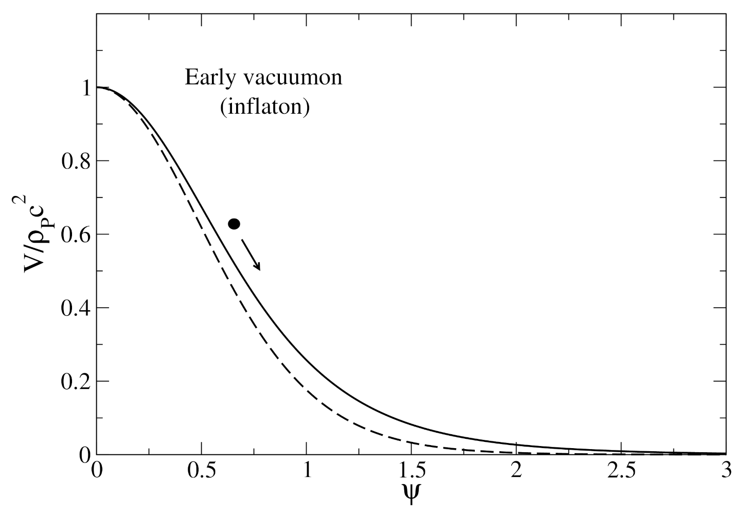
5.2. Early Vacuumon (Inflaton)

In the early universe (${\Omega }_{\Lambda }=0$), Equations (102) and (103) reduce to

$$\begin{array}{c}\hfill \varphi \left(a\right)={\left(\frac{3c^2}{8\pi G}\right)}^{1/2}\sqrt{1+\alpha }{\int }_0^a\frac{{\left(\frac{{\Omega }_{P,0}}{{\Omega }_{\alpha ,0}}\right)}^{1/2}{x}^{3(\alpha +1)/2}}{\sqrt{1+\frac{{\Omega }_{P,0}}{{\Omega }_{\alpha ,0}}{x}^{3(\alpha +1)}}}\frac{dx}{x},\end{array}$$

(111)

$$\begin{array}{c}\hfill \frac{V\left(a\right)}{{\rho }_0{c}^2}=\frac{1}{2}{\Omega }_{P,0}\frac{2+(1-\alpha )\frac{{\Omega }_{P,0}}{{\Omega }_{\alpha ,0}}{a}^{3(\alpha +1)}}{{\left(\frac{{\Omega }_{P,0}}{{\Omega }_{\alpha ,0}}{a}^{3(\alpha +1)}+1\right)}^2}.\end{array}$$

(112)

Introducing the notations from Equation (104), we find

$$\psi ={\int }_0^x\frac{ds}{{(1+s^2)}^{1/2}}={sinh}^{-1}\left(x\right),$$

(113)

$$V=\frac{1}{2}{\rho }_P{c}^2\frac{2+(1-\alpha )x^2}{{(x^2+1)}^2},$$

(114)

which corresponds to Equations (106) and (107) with $\kappa =0$. This returns Equations (122) and (123) of [44]. Eliminating x between these equations we obtain [44]

$$\begin{array}{c}\hfill V\left(\psi \right)=\frac{1}{2}{\rho }_P{c}^2\frac{(1-\alpha ){cosh}^2\psi +\alpha +1}{{cosh}^4\psi }(\psi \ge 0).\end{array}$$

(115)

This is the potential of the vacuumon in the early universe (playing the role of the inflaton). It is associated to the equation of state (49) valid in the early universe (see Section 8.1 of [42]). For $\psi \to 0$, it can be expanded in Taylor series as

$$\frac{V\left(\psi \right)}{{\rho }_P{c}^2}\simeq 1-\frac{3+\alpha }{2}{\psi }^2+\frac{9+5\alpha }{6}{\psi }^4+\dots$$

(116)

For $\psi \to +\infty$, we obtain the exponential asymptotic behaviors

$$\frac{V\left(\psi \right)}{{\rho }_P{c}^2}\sim 2(1-\alpha )e^{-2\psi },(\alpha \ne 1),$$

(117)

$$\frac{V\left(\psi \right)}{{\rho }_P{c}^2}\sim 16e^{-4\psi },(\alpha =1).$$

(118)

We note that the coefficient $\alpha =1$ (stiff matter) plays a special role as it leads to a faster decay of the potential. In that case [45,46]

$$\begin{array}{c}\hfill V\left(\psi \right)=\frac{{\rho }_P{c}^2}{{cosh}^4\psi }(\alpha =1).\end{array}$$

(119)

For the coefficient $\alpha =1/3$ (radiation), we have [42]

$$\begin{array}{c}\hfill V\left(\psi \right)=\frac{1}{3}{\rho }_P{c}^2\frac{{cosh}^2\psi +2}{{cosh}^4\psi }(\alpha =1/3).\end{array}$$

(120)

For $\alpha =0$ (pressureless matter), we have [42]

$$\begin{array}{c}\hfill V\left(\psi \right)=\frac{1}{2}{\rho }_P{c}^2\frac{{cosh}^2\psi +1}{{cosh}^4\psi }(\alpha =0).\end{array}$$

(121)

The potentials corresponding to $\alpha =1/3$ and $\alpha =1$ (relevant in the early universe) are plotted in Figure 1.

Recalling that $x={(a/a_1)}^{3(\alpha +1)/2}$ and using Equation (113), the relation between the scalar field and the scale factor is

$${(a/a_1)}^{3(\alpha +1)/2}=sinh\psi .$$

(122)

We can then express all the parameters of Section 3.2 as a function of $\psi$ instead of a. In particular, the energy density and the pressure of the scalar field are given by

$$\begin{array}{c}\hfill {\rho }_{\varphi }=\frac{{\rho }_P}{{cosh}^2\psi },\frac{P_{\varphi }}{{\rho }_P{c}^2}=\frac{\alpha {sinh}^2\psi -1}{{cosh}^4\psi }.\end{array}$$

(123)

The temporal evolution of the scalar field is discussed in detail in our previous papers [39,40,41,42,43,44,45,46,47]. According to Equations (59) and (122) we have

$$cosh\psi -ln\left(\frac{1+cosh\psi }{sinh\psi }\right)=\frac{3}{2}(\alpha +1){\left(\frac{8\pi }{3}\right)}^{1/2}\frac{t}{t_P}+C.$$

(124)

Remark 1.

For $a\to 0$, we can simplify Equation (111) into

$$\begin{array}{c}\hfill \varphi \left(a\right)={\left(\frac{3c^2}{8\pi G}\right)}^{1/2}\sqrt{1+\alpha }{\int }_0^a{\left(\frac{{\Omega }_{P,0}}{{\Omega }_{\alpha ,0}}\right)}^{1/2}{x}^{3(\alpha +1)/2}\frac{dx}{x},\end{array}$$

(125)

yielding

$$\begin{array}{c}\hfill \varphi \left(a\right)=\frac{2}{3}{\left(\frac{3c^2}{8\pi G}\right)}^{1/2}\frac{1}{\sqrt{1+\alpha }}{\left(\frac{{\Omega }_{P,0}}{{\Omega }_{\alpha ,0}}\right)}^{1/2}{a}^{\frac{3}{2}(1+\alpha )}.\end{array}$$

(126)

Substituting Equation (126) into Equation (112) we obtain the quadratic potential

$$\begin{array}{c}\hfill \frac{V\left(\varphi \right)}{{\rho }_0{c}^2}={\Omega }_{P,0}-\frac{3\pi G}{c^2}(1+\alpha )(3+\alpha ){\Omega }_{P,0}{\varphi }^2.\end{array}$$

(127)

This corresponds to the first term in the expansion of the potential from Equation (116).

5.3. Late Vacuumon (Quintessence)

In the late universe (${\Omega }_P\to +\infty$), Equations (102) and (103) reduce to

$$\begin{array}{c}\hfill \varphi \left(a\right)={\left(\frac{3c^2}{8\pi G}\right)}^{1/2}\sqrt{1+\alpha }{\int }^a\frac{1}{\sqrt{1+\frac{{\Omega }_{\Lambda ,0}}{{\Omega }_{\alpha ,0}}{x}^{3(\alpha +1)}}}\frac{dx}{x},\end{array}$$

(128)

$$\begin{array}{c}\hfill \frac{V\left(a\right)}{{\rho }_0{c}^2}=\frac{(1-\alpha ){\Omega }_{\alpha ,0}}{2a^{3(\alpha +1)}}+{\Omega }_{\Lambda ,0}.\end{array}$$

(129)

These expressions are valid for sufficiently large values of a. Introducing the notations from Equations (104) and (105), we find

$$\psi ={\int }^x\frac{ds}{s{(1+\kappa s^2)}^{1/2}}=-{sinh}^{-1}\left(\frac{1}{\sqrt{\kappa }x}\right)+{\psi }_{\max },$$

(130)

$$V=\frac{1}{2}{\rho }_P{c}^2\left(\frac{1-\alpha }{x^2}+2\kappa \right),$$

(131)

which correspond to Equations (106) and (107) with $x\gg 1$. Here, ${\psi }_{\max }$ appears as a constant of integration that can be obtained by matched asymptotics (see below). We recover Equations (125) and (126) of [44]. Eliminating x between these equations we obtain [44]

$$\begin{array}{c}\hfill V\left(\psi \right)=\frac{1}{2}{\rho }_{\Lambda }{c}^2\left[(1-\alpha ){cosh}^2({\psi }_{\max }-\psi )+\alpha +1\right](\psi \le {\psi }_{\max }).\end{array}$$

(132)

This is the potential of the vacuumon in the late universe (playing the role of the quintessence). It is associated to the equation of state (61) valid in the late universe (see Section 8.1. of [42]). For $\psi \to {\psi }_{\max }$, it can be expanded in Taylor series as

$$\frac{V\left(\psi \right)}{{\rho }_{\Lambda }{c}^2}\simeq 1+\frac{1-\alpha }{2}{({\psi }_{\max }-\psi )}^2+\frac{1-\alpha }{6}{({\psi }_{\max }-\psi )}^4+\dots$$

(133)

For $\psi \to -\infty$, we obtain the exponential asymptotic behavior

$$\frac{V\left(\psi \right)}{{\rho }_{\Lambda }{c}^2}\simeq \frac{1}{8}(1-\alpha )e^{2({\psi }_{\max }-\psi )},(\alpha \ne 1).$$

(134)

For $\alpha =1$ (stiff matter), the scalar field potential is constant

$$V\left(\psi \right)={\rho }_{\Lambda }{c}^2(\alpha =1).$$

(135)

For $\alpha =1/3$ (radiation), we have

$$V\left(\psi \right)=\frac{1}{2}{\rho }_{\Lambda }{c}^2\left[\frac{2}{3}{cosh}^2({\psi }_{\max }-\psi )+\frac{4}{3}\right](\alpha =1/3).$$

(136)

For $\alpha =0$ (pressureless matter), we have

$$V\left(\psi \right)=\frac{1}{2}{\rho }_{\Lambda }{c}^2\left[{cosh}^2({\psi }_{\max }-\psi )+1\right](\alpha =0).$$

(137)

The potential corresponding to $\alpha =0$ (relevant in the late universe) is plotted in Figure 2. This is the scalar field potential associated with the $\Lambda$CDM model viewed as a UDM model described by the constant equation of state $P_{\varphi }=-{\rho }_{\Lambda }{c}^2$.

Noting that $x\sqrt{\kappa }={(a/a_2)}^{3(\alpha +1)/2}$, where $a_2$ is defined by Equation (64), and using Equation (130), the relation between the scalar field and the scale factor is

$${(a_2/a)}^{3(\alpha +1)/2}=sinh({\psi }_{\max }-\psi ).$$

(138)

We can then express all the parameters of Section 3.3 as a function of $\psi$ instead of a. In particular, the energy density and the pressure of the scalar field are given by

$$\begin{array}{c}\hfill {\rho }_{\varphi }={\rho }_{\Lambda }{cosh}^2({\psi }_{\max }-\psi ),\frac{P_{\varphi }}{{\rho }_{\Lambda }{c}^2}=\alpha {sinh}^2({\psi }_{\max }-\psi )-1.\end{array}$$

(139)

The temporal evolution of the scalar field is discussed in detail in our previous papers [39,40,41,42,43,44,45,46,47]. According to Equations (71) and (138) we have

$${\psi }_{\max }-\psi ={sinh}^{-1}\left\{1/sinh\left[\frac{3}{2}(1+\alpha ){\left(\frac{8\pi }{3}\right)}^{1/2}\frac{t}{t_{\Lambda }}\right]\right\}.$$

(140)

Remark 2.

For $a\to +\infty$, we can simplify Equation (128) into

$$\begin{array}{c}\hfill \varphi \left(a\right)={\varphi }_{\max }-{\left(\frac{3c^2}{8\pi G}\right)}^{1/2}\sqrt{1+\alpha }{\int }_a^{+\infty }\frac{1}{\sqrt{\frac{{\Omega }_{\Lambda ,0}}{{\Omega }_{\alpha ,0}}{x}^{3(1+\alpha )}}}\frac{dx}{x},\end{array}$$

(141)

yielding

$$\begin{array}{c}\hfill \varphi \left(a\right)={\varphi }_{\max }-\frac{2}{3}{\left(\frac{3c^2}{8\pi G}\right)}^{1/2}\frac{1}{\sqrt{1+\alpha }}{\left(\frac{{\Omega }_{\alpha ,0}}{{\Omega }_{\Lambda ,0}}\right)}^{1/2}\frac{1}{a^{\frac{3}{2}(1+\alpha )}}.\end{array}$$

(142)

Substituting Equation (142) into Equation (129) we obtain the quadratic potential

$$\begin{array}{c}\hfill \frac{V\left(\varphi \right)}{{\rho }_0{c}^2}={\Omega }_{\Lambda ,0}+\frac{3\pi G}{c^2}(1-\alpha )(1+\alpha ){\Omega }_{\Lambda ,0}{({\varphi }_{\max }-\varphi )}^2.\end{array}$$

(143)

This corresponds to the first term in the expansion of the potential from Equation (133).

5.4. Matched Asymptotics

Using matched asymptotics, we find that the potential [44]

$$\begin{array}{ccc}\hfill V_{\mathrm{approx}}\left(\psi \right)& =& \frac{1}{2}{\rho }_P{c}^2\frac{(1-\alpha ){cosh}^2\psi +\alpha +1}{{cosh}^4\psi }\hfill \\ & +& \frac{1}{2}{\rho }_{\Lambda }{c}^2\left[(1-\alpha ){cosh}^2({\psi }_{\max }-\psi )+\alpha +1\right]\hfill \\ & -& 2{\rho }_P{c}^2(1-\alpha )e^{-2\psi }(0\le \psi \le {\psi }_{\max })\hfill \end{array}$$

(144)

provides a good approximation of the exact vacuumon potential given by Equation (108). It unifies the inflaton potential in the early universe (early vacuumon) and the quintessence potential in the late universe (late vacuumon) defined by Equations (115) and (132) respectively. In addition, matched asymptotics provides the value of the constant of integration ${\psi }_{\max }$ that appears in Equation (130). Indeed, by comparing Equations (117) and (134) we obtain ${\psi }_{\max }\simeq (1/2)ln(16/\kappa )=142.84\dots$ [44] in perfect agreement with the asymptotic expression of the exact value ${\psi }_{\max }=K(1-\kappa )$ for $\kappa \ll 1$ (see Section 5.1).

Remark 3.

For $\alpha =1$, the approximate potential from Equation (144) takes the particularly simple form

$$\begin{array}{c}\hfill V_{\mathrm{approx}}\left(\psi \right)=\frac{{\rho }_P{c}^2}{{cosh}^4\psi }+{\rho }_{\Lambda }{c}^2(\alpha =1).\end{array}$$

(145)

5.5. Intermediate Regime

In the intermediate regime valid after the early inflation and before the late accelerating expansion of the universe (${\Omega }_P\to +\infty$ and ${\Omega }_{\Lambda }=0$), the scalar field is described by the linear equation of state (73). In that case, Equations (102) and (103) reduce to

$$\begin{array}{c}\hfill \varphi \left(a\right)={\left(\frac{3c^2}{8\pi G}\right)}^{1/2}\sqrt{1+\alpha }{\int }^a\frac{dx}{x},\end{array}$$

(146)

$$\begin{array}{c}\hfill \frac{V\left(a\right)}{{\rho }_0{c}^2}=\frac{1}{2}(1-\alpha )\frac{{\Omega }_{\alpha ,0}}{a^{3(\alpha +1)}}.\end{array}$$

(147)

These equations can also be obtained from Equations (111) and (112) with ${\Omega }_P\to +\infty$ or from Equations (128) and (129) with ${\Omega }_{\Lambda }=0$. Integrating Equation (146), we obtain

$$\begin{array}{c}\hfill \varphi ={\left(\frac{3c^2}{8\pi G}\right)}^{1/2}\sqrt{1+\alpha }lna+{\varphi }_{\ast },\end{array}$$

(148)

where ${\varphi }_{\ast }$ is a constant of integration. Combining Equations (147) and (148), we obtain the exponential potential

$$\begin{array}{c}\hfill \frac{V\left(\varphi \right)}{{\rho }_0{c}^2}=\frac{1}{2}(1-\alpha ){\Omega }_{\alpha ,0}{e}^{-3{\left(\frac{8\pi G}{3c^2}\right)}^{1/2}\sqrt{1+\alpha }(\varphi -{\varphi }_{\ast })}.\end{array}$$

(149)

This result is equivalent to Equations (117) and (134) obtained long after the primordial inflation or long before the late accelerating expansion of the universe. This determines the constant of integration ${\psi }_{\ast }=(1/2)ln(4{\Omega }_{P,0}/{\Omega }_{\alpha ,0})$. For $\alpha =1$ (stiff matter), we find

$$\begin{array}{c}\hfill \varphi ={\left(\frac{3c^2}{8\pi G}\right)}^{1/2}\sqrt{2}lna+{\varphi }_{\ast },V\left(\varphi \right)=0(\alpha =1),\end{array}$$

(150)

corresponding to the regime of kination where the potential vanishes. Comparing Equation (150) with Equations (118) and (135) we see that the limits $\alpha \to 1$ and $\varphi \to \pm \infty$ do not commute. For $\alpha =-1$ (vacuum energy), we find

$$\begin{array}{c}\hfill \varphi ={\varphi }_{\ast },V\left(\varphi \right)={\rho }_{\ast }{c}^2(\alpha =-1),\end{array}$$

(151)

corresponding to the de Sitter regime where $\dot{\varphi }=0$.

Combining Equations (73), (76), and (148), we can express the density and the pressure as a function of the scalar field as

$$\begin{array}{c}\hfill P_{\varphi }=\alpha {\rho }_{\varphi }{c}^2=\alpha {\Omega }_{\alpha ,0}{\rho }_0{c}^2{e}^{-3\sqrt{\alpha +1}{\left(\frac{8\pi G}{3c^2}\right)}^{1/2}(\varphi -{\varphi }_{\ast })}.\end{array}$$

(152)

According to Equations (78) and (148), the temporal evolution of the scalar field is

$$\begin{array}{c}\hfill \varphi \left(t\right)={\left(\frac{3c^2}{8\pi G}\right)}^{1/2}\frac{2}{3\sqrt{1+\alpha }}ln\left[\frac{3}{2}(1+\alpha ){\left(\frac{8\pi G{\rho }_0{\Omega }_{\alpha ,0}}{3}\right)}^{1/2}t\right]+{\varphi }_{\ast }.\end{array}$$

(153)

5.6. Constant Scalar Field Potential

We have found different solutions corresponding to a constant scalar field potential (see Equations (135), (150) and (151)):

(i)

For the equation of state $P_{\varphi }={\rho }_{\varphi }{c}^2$ of stiff matter ($\alpha =1$), we have (see Section 3.4 and Section 5.5)

$$\begin{array}{c}\hfill {\rho }_{\varphi }\propto \frac{1}{a^6},a\propto t^{1/3},{\rho }_{\varphi }=\frac{1}{24\pi G{t}^2},\end{array}$$

(154)

$$\begin{array}{c}\hfill V\left(\varphi \right)=0,\varphi ={\left(\frac{3c^2}{4\pi G}\right)}^{1/2}lna+{\varphi }_{\ast },\varphi ={\left(\frac{c^2}{12\pi G}\right)}^{1/2}lnt+\mathrm{cst}.\end{array}$$

(155)

This solution describes a pure stiff matter era.

(ii)

For the equation of state $P_{\varphi }=-{\rho }_{\varphi }{c}^2$ of vacuum or dark energy ($\alpha =-1$), we have (see Section 3.4 and Section 5.5)

$$\begin{array}{c}\hfill {\rho }_{\varphi }=\mathrm{cst},a\propto e^{{\left(\frac{8\pi G{\rho }_{\varphi }}{3}\right)}^{1/2}t},V\left(\varphi \right)=\mathrm{cst},\varphi =\mathrm{cst}.\end{array}$$

(156)

This solution describes a pure de Sitter era.

(iii)

For the affine equation of state $P_{\varphi }={\rho }_{\varphi }{c}^2-2{\rho }_{\Lambda }{c}^2$, we have (see Section 3.3 and Section 5.3)

$$\begin{array}{ccc}\hfill \frac{{\rho }_{\varphi }}{{\rho }_{\Lambda }}=\frac{1}{{(a/a_2)}^6}+1,\frac{a}{a_2}& =& {sinh}^{1/3}\left[3{\left(\frac{8\pi }{3}\right)}^{1/2}\frac{t}{t_{\Lambda }}\right],\hfill \\ \hfill \frac{{\rho }_{\varphi }}{{\rho }_{\Lambda }}& =& \frac{1}{{tanh}^2\left[3{\left(\frac{8\pi }{3}\right)}^{1/2}\frac{t}{t_{\Lambda }}\right]},\hfill \end{array}$$

(157)

$$\begin{array}{c}\hfill V\left(\psi \right)={\rho }_{\Lambda }{c}^2,{\psi }_{\max }-\psi ={sinh}^{-1}\left[{\left(\frac{a_2}{a}\right)}^3\right],\\ \hfill {\psi }_{\max }-\psi ={sinh}^{-1}\left\{1/sinh\left[3{\left(\frac{8\pi }{3}\right)}^{1/2}\frac{t}{t_{\Lambda }}\right]\right\}.\end{array}$$

(158)

This solution describes a stiff matter era followed by a de Sitter era (late inflation).16 Therefore, several laws of evolution may correspond to the same potential.

6. Parameters of the Scalar Field

In this section, we determine the parameters (mass, self-interaction constant, and scattering length) of the scalar field in the early and late universe by comparing the form of the potential close to its maximum and minimum with the normal form of a quartic potential given by Equation (A54).

6.1. Early Vacuumon (Inflaton)

In the early universe, the potential of the vacuumon is given by Equation (115). For $\psi \to 0$, it can be expanded up to fourth order yielding Equation (116). Comparing Equation (116) with Equation (A54), we obtain the following results (see Appendix D):

(i)

The maximum value of the potential (corresponding to $\psi =0$) is equal to the Planck energy density

$$\begin{array}{c}\hfill V_{\max }={\rho }_P{c}^2,\end{array}$$

(159)

where ${\rho }_P=c^5/\hslash G^2=5.16\times {10}^{99}\mathrm{g}{\mathrm{m}}^{-3}$ is the Planck density.

(ii)

The squared mass of the scalar field is given by

$$\begin{array}{c}\hfill m^2=f_e\left(\alpha \right)\frac{8\pi }{3}{M}_P^2\end{array}$$

(160)

with

$$\begin{array}{c}\hfill f_e\left(\alpha \right)=-\frac{9}{4}(\alpha +1)(\alpha +3).\end{array}$$

(161)

We find $f_e=-27/4$ for $\alpha =0$, $f_e=-10$ for $\alpha =1/3$, and $f_e=-18$ for $\alpha =1$. The mass of the early vacuumon (inflaton) is imaginary ($f_e<0$) and its modulus $\left|m\right|$ is of the order of the Planck mass $M_P={\left(\hslash c/G\right)}^{1/2}=2.18\times {10}^{-5}\mathrm{g}=1.22\times {10}^{19}\mathrm{GeV}/{\mathrm{c}}^2$.

(iii)

The dimensionless self-interaction constant of the scalar field is given by

$$\begin{array}{c}\hfill \frac{\lambda }{8\pi }=g_e\left(\alpha \right)3\pi \end{array}$$

(162)

with

$$\begin{array}{c}\hfill g_e\left(\alpha \right)={(\alpha +1)}^2(9+5\alpha ).\end{array}$$

(163)

We find $g_e=9$ for $\alpha =0$, $g_e=512/27$ for $\alpha =1/3$, and $g_e=56$ for $\alpha =1$. The self-interaction constant of the early vacuumon (inflaton) is positive ($g_e>0$), corresponding to a repulsive self-interaction of order 1.

(iv)

The dimensional self-interaction constant of the scalar field is given by

$$\begin{array}{c}\hfill {\lambda }_s=\frac{27\pi }{4}\frac{g_e\left(\alpha \right)}{|f_e\left(\alpha \right)|}\frac{G{\hslash }^2}{c^2}.\end{array}$$

(164)

We find $g_e/\left|f_e\right|=4/3$ for $\alpha =0$, $g_e/\left|f_e\right|=256/135$ for $\alpha =1/3$, and $g_e/\left|f_e\right|=28/9$ for $\alpha =1$. The dimensional self-interaction constant of the early vacuumon (inflaton) is of order $G{\hslash }^2/c^2=5.15\times {10}^{-71}\mathrm{eV}{\mathrm{cm}}^3$.

(v)

The scattering length of the bosons associated with the scalar field is given by

$$\begin{array}{c}\hfill a_s=\frac{27}{32}\frac{g_e\left(\alpha \right)}{\sqrt{|f_e\left(\alpha \right)|}}2\sqrt{\frac{8\pi }{3}}{l}_P.\end{array}$$

(165)

We find $g_e^2/\left|f_e\right|=12$ for $\alpha =0$, $g_e^2/\left|f_e\right|=131072/3645$ for $\alpha =1/3$, and $g_e^2/\left|f_e\right|=1568/9$ for $\alpha =1$. The scattering length $a_s$ of the bosons associated with the early vacuumon (inflaton) is of the order of the Planck length $l_P=G{M}_P/c^2={(G\hslash /c^3)}^{1/2}=1.62\times {10}^{-35}\mathrm{m}$ which corresponds to the semi Schwarzschild radius associated with the Planck mass $M_P$.

In theories of extended supergravity, the mass of a scalar field is quantized according to the rule [66]

$$m^2=n_{\ast }\frac{H^2{\hslash }^2}{c^4},$$

(166)

where $n_{\ast }$ is an integer and H is the Hubble factor in the de Sitter era. As $H^2=8\pi G{\rho }_P/3$ during the early inflation, we can rewrite Equation (166) as

$$m^2=n_{\ast }\frac{8\pi G{\rho }_P{\hslash }^2}{3c^4}=n_{\ast }\frac{8\pi }{3}{M}_P^2.$$

(167)

The quantum of mass ($n_{\ast }=1$) in the early universe is the rescaled Planck mass $M_P^{\ast }=\sqrt{8\pi /3}{M}_P$. Comparing Equation (167) with Equation (160), the quantization rule implies that $f_e\left(\alpha \right)$ should be an integer $n_{\ast }$. We see that this quantization rule is realized for the integer value $n_{\ast }=-10$ when $\alpha =1/3$ (radiation) and for the integer value $n_{\ast }=-18$ when $\alpha =1$ (stiff) [47,67]. By contrast, $f_e\left(\alpha \right)$ is not an integer when $\alpha =0$ (matter). This may be connected to the fact that the index $\alpha =0$ is not justified in the early universe as there is no matter there in the usual sense.

6.2. Late Vacuumon (Quintessence)

In the late universe, the potential of the vacuumon is given by Equation (132). For $\psi \to {\psi }_{\max }$, it can be expanded up to fourth order yielding Equation (133).17 Comparing Equation (133) with Equation (A54), with the substitution $\varphi \to {\varphi }_{\max }-\varphi$, we obtain the following results (see Appendix D):

(i)

The minimum value of the potential (corresponding to $\psi ={\psi }_{\max }$) is equal to the cosmological energy density

$$\begin{array}{c}\hfill V_{\min }={\rho }_{\Lambda }{c}^2,\end{array}$$

(168)

where ${\rho }_{\Lambda }=\Lambda /8\pi G=5.96\times {10}^{-24}\mathrm{g}{\mathrm{m}}^{-3}$ is the cosmological density.

(ii)

The squared mass of the scalar field is given by

$$\begin{array}{c}\hfill m^2=f_l\left(\alpha \right)\frac{1}{3}{m}_{\Lambda }^2\end{array}$$

(169)

with

$$\begin{array}{c}\hfill f_l\left(\alpha \right)=\frac{9}{4}(\alpha +1)(1-\alpha ).\end{array}$$

(170)

We find $f_l=9/4$ for $\alpha =0$, $f_l=2$ for $\alpha =1/3$, and $f_l=0$ for $\alpha =1$. The mass of the late vacuumon (quintessence) is real ($f_l>0$) and of the order of the cosmon mass $m_{\Lambda }=\hslash \sqrt{\Lambda }/c^2=2.08\times {10}^{-33}\mathrm{eV}/{\mathrm{c}}^2$, except for $\alpha =1$ (stiff matter) where $m=0$. Our approach provides therefore a physical interpretation of the cosmon mass as being the mass of the scalar field responsible for the dark energy in the late universe. To the best of our knowledge, this interpretation has not been given before.

(iii)

The dimensionless self-interaction constant of the scalar field is given by

$$\begin{array}{c}\hfill \frac{\lambda }{8\pi }=g_l\left(\alpha \right)3\pi \frac{{\rho }_{\Lambda }}{{\rho }_P}\end{array}$$

(171)

with

$$\begin{array}{c}\hfill g_l\left(\alpha \right)={(\alpha +1)}^2(1-\alpha ).\end{array}$$

(172)

We find $g_l=1$ for $\alpha =0$, $g_l=32/27$ for $\alpha =1/3$, and $g_l=0$ for $\alpha =1$. The self-interaction constant of the late vacuumon (quintessence) is positive ($g_l>0$), corresponding to a repulsive self-interaction of order ${\rho }_{\Lambda }/{\rho }_P\sim {10}^{-123}$, except for $\alpha =1$ (stiff matter) where $\lambda =0$.

(iv)

The dimensional self-interaction constant of the scalar field is given by

$$\begin{array}{c}\hfill {\lambda }_s=\frac{27\pi }{4}\frac{g_l\left(\alpha \right)}{f_l\left(\alpha \right)}\frac{G{\hslash }^2}{c^2}.\end{array}$$

(173)

We find $g_l/f_l=4/9$ for $\alpha =0$, $g_l/f_l=16/27$ for $\alpha =1/3$, and $g_l/f_l\to 8/9$ for $\alpha \to 1$. The dimensional self-interaction constant of the late vacuumon (quintessence) is of order $G{\hslash }^2/c^2=5.15\times {10}^{-71}\mathrm{eV}{\mathrm{cm}}^3$, except for $\alpha =1$ (stiff matter) where ${\lambda }_s=0$ (note that the result obtained in the limit $\alpha \to 1$ is different from the result obtained for $\alpha =1$).

(v)

The scattering length of the bosons associated with the scalar field is given by

$$\begin{array}{c}\hfill a_s=\frac{27}{32}\frac{g_l\left(\alpha \right)}{\sqrt{f_l\left(\alpha \right)}}\frac{2}{\sqrt{3}}{r}_{\Lambda }.\end{array}$$

(174)

We find $g_l/\sqrt{f_l}=2/3$ for $\alpha =0$, $g_l/\sqrt{f_l}=16\sqrt{2}/27$ for $\alpha =1/3$, and $g_l/\sqrt{f_l}\to 0$ for $\alpha \to 1$. The scattering length $a_s$ of the bosons associated with the late vacuumon (quintessence) is of the order of the cosmon radius $r_{\Lambda }=G{m}_{\Lambda }/c^2=G\hslash \sqrt{\Lambda }/c^4=2.75\times {10}^{-96}\mathrm{m}$, which corresponds to the semi Schwarzschild radius associated with the cosmon mass $m_{\Lambda }$, except for $\alpha =1$ (stiff matter) where $a_s=0$.

As $H^2=8\pi G{\rho }_{\Lambda }/3$ during the late inflation, we can rewrite the quantization rule (166) as

$$m^2=n_{\ast }\frac{8\pi G{\rho }_{\Lambda }{\hslash }^2}{3c^4}=n_{\ast }\frac{1}{3}{m}_{\Lambda }^2.$$

(175)

The quantum of mass $(n_{\ast }=1$) in the late universe is the rescaled cosmon mass $m_{\Lambda }^{\ast }=\frac{1}{\sqrt{3}}{m}_{\Lambda }$.18 Comparing Equation (169) with Equation (175), the quantization rule implies that $f_l\left(\alpha \right)$ should be an integer $n_{\ast }$. We see that this quantization rule is realized for the integer value $n_{\ast }=2$ when $\alpha =1/3$ (radiation) and for the integer value $n_{\ast }=0$ when $\alpha =1$ (stiff matter) [47,67]. By contrast, $f_l\left(\alpha \right)$ is not an integer when $\alpha =0$ (matter). We recall that our model of late universe with $\alpha =0$ is equivalent to the $\Lambda$CDM model interpreted as a UDM model. Therefore, the quintessence field associated with the standard $\Lambda$CDM model ($\alpha =0$) does not satisfy the quantization rule (166) [47,67]. This suggests (provided that this quantization rule must hold, which is not firmly established) that the relevant value of $\alpha$ to take is $\alpha =1/3$ or $\alpha =1$, and that dark matter should be treated as an independent species, as in scenario (B).

Remark 4.

In this paper, we have described the late universe by a polytrope of index $n=-1$ [42]. For $\alpha =0$ and $n=-1$, our model is equivalent to the ΛCDM model. If we consider a more general polytropic equation of state with $\alpha =0$ and an arbitrary index $n<0$ (see Equation (A45) and Ref. [42]), we find that the mass of the scalar field in the late universe is given by (see Appendix D and [47,67])

$$m^2=-\frac{1+2n}{n^2}\frac{6\pi G{\rho }_{\Lambda }{\hslash }^2}{c^4}.$$

(176)

We note that this mass presents a maximum as a function of n for $n=-1$. Interestingly, this maximum selects the ΛCDM model among all the polytropic models of the form of Equation (A45) with $\alpha =0$ and $n<0$ [47,67].

7. Scalar Field in the Presence of One Fluid in the Intermediate Regime

7.1. General Results

In this section, we consider the complete model of Section 4 in the intermediate regime between the two de Sitter eras. In this regime, the scalar field has a linear equation of state $P_{\varphi }=\alpha {\rho }_{\varphi }{c}^2$. We use approach (B) in which the value of $\alpha$ is fixed. As we have seen, relevant values of $\alpha$ are $\alpha =1$ (stiff matter) or $\alpha =1/3$ (radiation). On the other hand, we have to take into account the presence of X-fluids which also have a linear equation of state $P_X={\alpha }_X{\rho }_X{c}^2$. If the scalar field evolves in the presence of radiation, one has ${\alpha }_r=1/3$. If it evolves in the presence of matter, one has ${\alpha }_m=0$. For the sake of generality, we consider arbitrary values of $\alpha$ and ${\alpha }_X$ but we assume that $\alpha \ge -1$ and ${\alpha }_X\ge -1$ so that the universe has not a phantom behavior.

The energy density of the scalar field and of the X-fluids evolve with the scale factor as

$$\begin{array}{c}\hfill \frac{{\rho }_{\varphi }}{{\rho }_0}=\frac{{\Omega }_{\alpha ,0}}{a^{3(1+\alpha )}},\frac{{\rho }_X}{{\rho }_0}=\frac{{\Omega }_{X,0}}{a^{3(1+{\alpha }_X)}}.\end{array}$$

(177)

The total energy density is therefore

$$\begin{array}{c}\hfill \frac{\rho }{{\rho }_0}=\sum _X\frac{{\Omega }_{X,0}}{a^{3(1+{\alpha }_X)}}+\frac{{\Omega }_{\alpha ,0}}{a^{3(1+\alpha )}}.\end{array}$$

(178)

The time evolution $a\left(t\right)$ of the scale factor is determined by the Friedmann equation

$$\begin{array}{c}\hfill H^2=\frac{8\pi G}{3}\rho =\frac{8\pi G}{3}\left(\sum _X{\rho }_X+{\rho }_{\varphi }\right),\end{array}$$

(179)

where the right hand side is given by Equation (178).19 On the other hand, the scalar field potential is determined by the equations20

$$\begin{array}{c}\hfill \varphi \left(a\right)={\left(\frac{3c^2}{8\pi G}\right)}^{1/2}\sqrt{1+\alpha }{\int }_0^a\sqrt{\frac{\frac{{\Omega }_{\alpha ,0}}{x^{3(\alpha +1)}}}{{\sum }_X\frac{{\Omega }_{X,0}}{x^{3(1+{\alpha }_X)}}+\frac{{\Omega }_{\alpha ,0}}{x^{3(\alpha +1)}}}}\frac{dx}{x},\end{array}$$

(180)

$$\begin{array}{c}\hfill \frac{V\left(a\right)}{{\rho }_0{c}^2}=\frac{1}{2}(1-\alpha ){\Omega }_{\alpha ,0}\frac{1}{a^{3(\alpha +1)}}.\end{array}$$

(181)

In the following, in order to have analytical results, we assume that there is just one X-fluid in addition to the scalar field. It can represent for example radiation (${\alpha }_X=1/3$) or matter (${\alpha }_X=0$). The case of two X-fluids (radiation and matter) in addition to the scalar field could be treated numerically. We obtain the form of the potential in the limiting case where one perfect fluid dominates over the other. In our model, the foregoing equations are valid only in the intermediate regime between the two de Sitter eras, where the equation of state of the scalar field can be approximated by a linear law, so they have a restricted domain of validity. However, in our mathematical analysis below, we shall study Equations (177)–(181) for all times because they can be relevant in other contexts, for example in the case where the fluid describes dark matter and the scalar field describes dark energy (see Section 7.3).

7.2. Hyperbolic Potential

We first assume $\alpha <{\alpha }_X$. In that case, the X-fluid dominates at early times and the scalar field dominates at late times. Equation (180) can be rewritten as

$$\begin{array}{c}\hfill \varphi \left(a\right)={\left(\frac{3c^2}{8\pi G}\right)}^{1/2}\sqrt{1+\alpha }{\int }_0^a\frac{dx}{x\sqrt{1+\frac{{\Omega }_{X,0}}{{\Omega }_{\alpha ,0}}\frac{1}{x^{3({\alpha }_X-\alpha )}}}}.\end{array}$$

(182)

Making the change of variables

$$\begin{array}{c}\hfill X=\frac{{\Omega }_{X,0}}{{\Omega }_{\alpha ,0}}\frac{1}{x^{3({\alpha }_X-\alpha )}},\end{array}$$

(183)

we obtain

$$\begin{array}{c}\hfill \varphi \left(a\right)={\left(\frac{3c^2}{8\pi G}\right)}^{1/2}\sqrt{1+\alpha }\frac{1}{3({\alpha }_X-\alpha )}{\int }_{\frac{{\Omega }_{X,0}}{{\Omega }_{\alpha ,0}}\frac{1}{a^{3({\alpha }_X-\alpha )}}}^{+\infty }\frac{dX}{X\sqrt{1+X}}.\end{array}$$

(184)

Using the identity

$$\begin{array}{c}\hfill \int \frac{1}{\sqrt{x+1}}\frac{dx}{x}=ln\left(\frac{\sqrt{1+x}-1}{\sqrt{1+x}+1}\right)=-2{sinh}^{-1}\left(\frac{1}{\sqrt{x}}\right),\end{array}$$

(185)

we find

$$\begin{array}{c}\hfill \varphi \left(a\right)={\left(\frac{3c^2}{8\pi G}\right)}^{1/2}\sqrt{1+\alpha }\frac{2}{3({\alpha }_X-\alpha )}{sinh}^{-1}\left[\sqrt{\frac{{\Omega }_{\alpha ,0}}{{\Omega }_{X,0}}}{a}^{\frac{3}{2}({\alpha }_X-\alpha )}\right].\end{array}$$

(186)

Inversely,

$$\begin{array}{c}\hfill a={\left(\frac{{\Omega }_{X,0}}{{\Omega }_{\alpha ,0}}\right)}^{\frac{1}{3({\alpha }_X-\alpha )}}{sinh}^{\frac{2}{3({\alpha }_X-\alpha )}}\left[{\left(\frac{8\pi G}{3c^2}\right)}^{1/2}\frac{1}{\sqrt{1+\alpha }}\frac{3({\alpha }_X-\alpha )}{2}\varphi \right].\end{array}$$

(187)

Combining Equation (187) with Equation (181), we obtain the hyperbolic potential

$$\begin{array}{ccc}\hfill V\left(\varphi \right)& =& \frac{1}{2}{\rho }_0{c}^2{\Omega }_{\alpha ,0}(1-\alpha ){\left(\frac{{\Omega }_{\alpha ,0}}{{\Omega }_{X,0}}\right)}^{\frac{\alpha +1}{{\alpha }_X-\alpha }}\hfill \\ & \times & {sinh}^{-\frac{2(\alpha +1)}{{\alpha }_X-\alpha }}\left[{\left(\frac{8\pi G}{3c^2}\right)}^{1/2}\frac{1}{\sqrt{1+\alpha }}\frac{3({\alpha }_X-\alpha )}{2}\varphi \right].\hfill \end{array}$$

(188)

We now assume $\alpha >{\alpha }_X$. In that case, the scalar field dominates at early times and the X-fluid dominates at late times. We note that the integral from Equation (182) diverges at $x=0$. We can easily circumvent this problem by redefining the additive constant in the scalar field so that

$$\begin{array}{c}\hfill \varphi \left(a\right)=-{\left(\frac{3c^2}{8\pi G}\right)}^{1/2}\sqrt{1+\alpha }{\int }_a^{+\infty }\frac{dx}{x\sqrt{1+\frac{{\Omega }_{X,0}}{{\Omega }_{\alpha ,0}}\frac{1}{x^{3({\alpha }_X-\alpha )}}}}.\end{array}$$

(189)

With this convention, we can check that the previous Equations (186)–(188) remain valid.

Finally, when $\alpha ={\alpha }_X$, Equation (180) reduces to

$$\begin{array}{c}\hfill \varphi \left(a\right)={\left(\frac{3c^2}{8\pi G}\right)}^{1/2}\sqrt{1+\alpha }\frac{1}{\sqrt{1+\frac{{\Omega }_{X,0}}{{\Omega }_{\alpha ,0}}}}{\int }_1^a\frac{dx}{x},\end{array}$$

(190)

where we have chosen the origin of the scalar field at $a=1$ in order to avoid spurious divergences. This yields

$$\begin{array}{c}\hfill \varphi \left(a\right)={\left(\frac{3c^2}{8\pi G}\right)}^{1/2}\sqrt{1+\alpha }{\left(\frac{{\Omega }_{\alpha ,0}}{{\Omega }_{X,0}+{\Omega }_{\alpha ,0}}\right)}^{1/2}lna.\end{array}$$

(191)

Inversely,

$$\begin{array}{c}\hfill a=e^{{\left(\frac{8\pi G}{3c^2}\right)}^{1/2}\frac{1}{\sqrt{1+\alpha }}{\left(\frac{{\Omega }_{X,0}+{\Omega }_{\alpha ,0}}{{\Omega }_{\alpha ,0}}\right)}^{1/2}\varphi }.\end{array}$$

(192)

Combining Equation (192) with Equation (181) we obtain the exponential potential

$$\begin{array}{c}\hfill \frac{V\left(\varphi \right)}{{\rho }_0{c}^2}=\frac{1}{2}(1-\alpha ){\Omega }_{\alpha ,0}{e}^{-3{\left(\frac{8\pi G}{3c^2}\right)}^{1/2}\sqrt{1+\alpha }{\left(\frac{{\Omega }_{X,0}+{\Omega }_{\alpha ,0}}{{\Omega }_{\alpha ,0}}\right)}^{1/2}\varphi }.\end{array}$$

(193)

For a scalar field alone (${\Omega }_{X,0}=0$) we recover Equation (149).

Below, we consider particular limits of the hyperbolic potential (188).

7.2.1. Power-Law Potential

When the terms in brackets in Equations (186)–(188) go to zero, we find

$$\begin{array}{c}\hfill \varphi \left(a\right)={\left(\frac{3c^2}{8\pi G}\right)}^{1/2}\sqrt{1+\alpha }\frac{2}{3({\alpha }_X-\alpha )}\sqrt{\frac{{\Omega }_{\alpha ,0}}{{\Omega }_{X,0}}}{a}^{\frac{3}{2}({\alpha }_X-\alpha )},\end{array}$$

(194)

$$\begin{array}{c}\hfill a={\left(\frac{{\Omega }_{X,0}}{{\Omega }_{\alpha ,0}}\right)}^{\frac{1}{3({\alpha }_X-\alpha )}}{\left[{\left(\frac{8\pi G}{3c^2}\right)}^{1/2}\frac{1}{\sqrt{1+\alpha }}\frac{3({\alpha }_X-\alpha )}{2}\varphi \right]}^{\frac{2}{3({\alpha }_X-\alpha )}},\end{array}$$

(195)

$$\begin{array}{c}\hfill V\left(\varphi \right)=\frac{1}{2}{\rho }_0{c}^2{\Omega }_{\alpha ,0}(1-\alpha ){\left(\frac{{\Omega }_{\alpha ,0}}{{\Omega }_{X,0}}\right)}^{\frac{\alpha +1}{{\alpha }_X-\alpha }}{\left[{\left(\frac{8\pi G}{3c^2}\right)}^{1/2}\frac{1}{\sqrt{1+\alpha }}\frac{3({\alpha }_X-\alpha )}{2}\varphi \right]}^{-\frac{2(\alpha +1)}{{\alpha }_X-\alpha }}.\end{array}$$

(196)

This corresponds to the situation where the X-fluid dominates the scalar field. In that case, we obtain a power-law potential. When $\alpha <{\alpha }_X$, this approximation is valid at sufficiently early times ($R\to 0$, $\varphi \to 0^{+}$ and $V\to +\infty$). When $\alpha >{\alpha }_X$, it is valid at sufficiently late times ($R\to +\infty$, $\varphi \to 0^{-}$ and $V\to 0$). Pure (inverse) power-law potentials were introduced by Peebles and Ratra [30,31]. They were used in relation to tracker solutions [22,23,33].

7.2.2. Exponential Potential

When the terms in brackets in Equations (186)–(188) go to $+\infty$, we find

$$\begin{array}{c}\hfill \varphi \left(a\right)={\left(\frac{3c^2}{8\pi G}\right)}^{1/2}\sqrt{1+\alpha }\frac{2}{3({\alpha }_X-\alpha )}ln\left[2\sqrt{\frac{{\Omega }_{\alpha ,0}}{{\Omega }_{X,0}}}{a}^{\frac{3}{2}({\alpha }_X-\alpha )}\right],\end{array}$$

(197)

$$\begin{array}{c}\hfill a={\left(\frac{{\Omega }_{X,0}}{{\Omega }_{\alpha ,0}}\right)}^{\frac{1}{3({\alpha }_X-\alpha )}}\frac{1}{2^{\frac{2}{3({\alpha }_X-\alpha )}}}{e}^{{\left(\frac{8\pi G}{3c^2}\right)}^{1/2}\frac{1}{\sqrt{1+\alpha }}\varphi },\end{array}$$

(198)

$$\begin{array}{c}\hfill V\left(\varphi \right)=\frac{1}{2}{\rho }_0{c}^2{\Omega }_{\alpha ,0}(1-\alpha ){\left(\frac{{\Omega }_{\alpha ,0}}{{\Omega }_{X,0}}\right)}^{\frac{\alpha +1}{{\alpha }_X-\alpha }}{2}^{\frac{2(\alpha +1)}{{\alpha }_X-\alpha }}{e}^{-3{\left(\frac{8\pi G}{3c^2}\right)}^{1/2}\sqrt{1+\alpha }\varphi }.\end{array}$$

(199)

This corresponds to the situation where the scalar field dominates the X-fluid. In that case, we obtain an exponential potential as when the scalar field with a linear equation of state is alone in the universe (see Section 5.5).21 When $\alpha <{\alpha }_X$, this approximation is valid at sufficiently late times ($R\to +\infty$, $\varphi \to +\infty$ and $V\to 0$). When $\alpha >{\alpha }_X$, it is valid at sufficiently early times ($R\to 0$, $\varphi \to -\infty$ and $V\to +\infty$). Pure exponential potentials were introduced by Halliwell [69] (see also [31,70,71,72,73,74,75]). Exponential potentials arise very naturally in all models of unification with gravity such as Kaluza–Klein theories, supergravity theory or string theory. Most theories undergoing dimensional reduction to an effective four-dimensional theory yield exponential potentials.

7.3. Comparison with Other Works

The hyperbolic potential (188) has been obtained by several authors [18,76,77,78,79,80,81] using different methods. In these models, the fluid characterized by an equation of state $P_X={\alpha }_X{\rho }_X{c}^2$ with $0\le {\alpha }_X\le 1$ describes radiation (${\alpha }_X=1/3$) or dark matter (${\alpha }_X=0$) and the scalar field characterized by an equation of state $P_{\varphi }=\alpha {\rho }_{\varphi }{c}^2$ with $-1<\alpha \le -1/3$ (e.g., $\alpha =-0.65$ [79] or $\alpha =-2/3$ [80]) describes DE. As $\alpha <{\alpha }_X$ these models describe a radiation or dark matter era followed by a dark energy era. During the radiation or dark matter era, the universe is decelerating and the scale factor increases algebraically as $t^{1/2}$ or $t^{2/3}$ (see Equation (23)). During the dark energy era, the universe is accelerating and the scale factor increases algebraically as $t^{2/\left[3\right(1+\alpha \left)\right]}$ (power-law inflation). In the radiation and dark matter eras, the scalar field is subdominant and the potential $V\left(\varphi \right)$ has an inverse power-law behavior (tracking). In the dark energy era, the scalar field dominates the other species (X-fluids) and the potential $V\left(\varphi \right)$ has an exponential behavior as when a scalar field with a linear equation of state is alone in the universe. We thus achieve a tracker solution that can drive the universe into its current inflationary state. The behavior of the potential as an inverse power-law potential at early times avoids the fine-tuning problem and the cosmic coincidence problem [22]. Its exponential behavior at late time drives the universe into a power-law inflationary stage in agreement with the observations. In this model, the scalar field describes only dark energy, and we have to add radiation and (dark) matter as additional species.

In the present work, the hyperbolic potential (188) is obtained in a particular limit of a more general model based on a scalar field with a quadratic equation of state in the presence of X-fluids. It is valid in the intermediate regime between the early and late inflation. The scalar field models dark radiation ($\alpha =1/3$) or stiff matter ($\alpha =1$) and the fluid models radiation (${\alpha }_X=1/3$) or matter (${\alpha }_X=0$). As $\alpha \ge {\alpha }_X$, we are always in the situation where the scalar field dominates at early times and the X-fluid dominates at late times (note that the scalar field dominates again in the late universe due to the constant term $-(\alpha +1){\rho }_{\Lambda }{c}^2$ in its equation of state which has been ignored in the intermediate regime). Therefore, in this intermediate period, the scalar field potential is initially exponential and then becomes algebraic.

Remark 5.

The ΛCDM model corresponds to ${\alpha }_X=0$ and $\alpha =-1$. In that case, $\varphi =\mathrm{cst}$ and $V\left(\varphi \right)=\mathrm{cst}$. The ΛCDM model can also be obtained by taking ${\alpha }_X=-1$ and $\alpha =0$. In that case, the scalar field has a potential

$$\begin{array}{c}\hfill V\left(\varphi \right)=\frac{1}{2}{\rho }_0{c}^2{\Omega }_{X,0}{sinh}^2\left[{\left(\frac{8\pi G}{3c^2}\right)}^{1/2}\frac{3}{2}\varphi \right].\end{array}$$

(200)

8. Scalar Field in the Presence of One Fluid in the Late Universe

In this section, we consider the complete model of Section 4 in the late universe (we consider just one X-fluid in addition to the scalar field). In that case, the scalar field has an affine equation of state $P_{\varphi }=\alpha {\rho }_{\varphi }{c}^2-(\alpha +1){\rho }_{\Lambda }{c}^2$. The scalar field potential is determined by Equations (98) and (99) which can be rewritten as

$$\begin{array}{c}\hfill \varphi \left(a\right)={\left(\frac{3c^2}{8\pi G}\right)}^{1/2}\sqrt{1+\alpha }{\int }^a\frac{1}{\sqrt{\frac{{\Omega }_{X,0}}{{\Omega }_{\alpha ,0}}{x}^{3(\alpha -{\alpha }_X)}+1+\frac{{\Omega }_{\Lambda ,0}}{{\Omega }_{\alpha ,0}}{x}^{3(1+\alpha )}}}\frac{dx}{x},\end{array}$$

(201)

$$\begin{array}{c}\hfill \frac{V\left(a\right)}{{\rho }_0{c}^2}=\frac{(1-\alpha ){\Omega }_{\alpha ,0}}{2a^{3(\alpha +1)}}+{\Omega }_{\Lambda ,0}.\end{array}$$

(202)

The scalar field is described by the index $\alpha =1/3$ (radiation) or $\alpha =1$ (stiff) and the X-fluid is described by the index ${\alpha }_X=0$ (matter). Unfortunately, the integral cannot be calculated analytically in general except in the degenerate case $\alpha ={\alpha }_X$ (see below) which is not relevant in our situation. However, in the very late universe, we can ignore the term in ${\Omega }_{X,0}$ in Equation (201). In that case, we are led back to the equations (128) and (129) valid for a scalar field alone in the universe leading to the potential from Equation (132). Note that for $\alpha =1$ (stiff matter), the potential from Equation (202) is constant:

$$\begin{array}{c}\hfill V\left(\varphi \right)={\rho }_{\Lambda }{c}^2(\alpha =1),\end{array}$$

(203)

whether or not an X-fluid is present. In addition, for $\alpha =1$ and ${\alpha }_X=0$ the integral in Equation (201) can be computed analytically, giving

$$\begin{array}{c}\hfill \varphi \left(a\right)=\frac{\sqrt{2}}{3}{\left(\frac{3c^2}{8\pi G}\right)}^{1/2}ln\left[\frac{a^3}{2+\frac{{\Omega }_{X,0}}{{\Omega }_{\alpha ,0}}{a}^3+2\sqrt{1+\frac{{\Omega }_{X,0}}{{\Omega }_{\alpha ,0}}{a}^3+\frac{{\Omega }_{\Lambda ,0}}{{\Omega }_{\alpha ,0}}{a}^6}}\right]+\mathrm{cst}.\end{array}$$

(204)

For $a\gg 1$, it reduces to

$$\begin{array}{c}\hfill \varphi \left(a\right)=-\frac{2\sqrt{2}}{3}{\left(\frac{3c^2}{8\pi G}\right)}^{1/2}\frac{{\Omega }_{\alpha ,0}}{{\Omega }_{X,0}}\sqrt{\frac{{\Omega }_{X,0}}{{\Omega }_{\alpha ,0}}\frac{1}{a^3}+\frac{{\Omega }_{\Lambda ,0}}{{\Omega }_{\alpha ,0}}}+\mathrm{cst}.\end{array}$$

(205)

This expression provides the correction to Equation (128) due to the presence of the X-fluid.

Remark 6.

It is interesting at a general level to consider the case $\alpha ={\alpha }_X$ in Equation (201) where the integral can be calculated analytically. This corresponds to a situation where a scalar field described by the affine equation of state $P_{\varphi }=\alpha {\rho }_{\varphi }{c}^2-(\alpha +1){\rho }_{\Lambda }{c}^2$ evolves in the presence of an X-fluid described by the linear equation of state $P_X={\alpha }_X{\rho }_X{c}^2$ with ${\alpha }_X=\alpha$.22 In that case, Equation (201) reduces to

$$\begin{array}{c}\hfill \varphi \left(a\right)=-{\left(\frac{3c^2}{8\pi G}\right)}^{1/2}\sqrt{1+\alpha }\frac{1}{\sqrt{\frac{{\Omega }_{X,0}}{{\Omega }_{\alpha ,0}}+1}}{\int }_a^{+\infty }\frac{1}{\sqrt{1+\frac{{\Omega }_{\Lambda ,0}}{{\Omega }_{X,0}+{\Omega }_{\alpha ,0}}{x}^{3(1+\alpha )}}}\frac{dx}{x},\end{array}$$

(206)

where we have chosen the origin of the scalar field at $a\to +\infty$ in order to avoid spurious divergences at $x=0$.23 Making the change of variables

$$\begin{array}{c}\hfill X=\frac{{\Omega }_{\Lambda ,0}}{{\Omega }_{X,0}+{\Omega }_{\alpha ,0}}{x}^{3(\alpha +1)},\end{array}$$

(207)

we obtain

$$\begin{array}{c}\hfill \varphi \left(a\right)=-{\left(\frac{3c^2}{8\pi G}\right)}^{1/2}\frac{1}{\sqrt{\frac{{\Omega }_{X,0}}{{\Omega }_{\alpha ,0}}+1}}\frac{1}{3\sqrt{\alpha +1}}{\int }_{\frac{{\Omega }_{\Lambda ,0}}{{\Omega }_{X,0}+{\Omega }_{\alpha ,0}}{a}^{3(\alpha +1)}}^{+\infty }\frac{1}{\sqrt{1+X}}\frac{dX}{X}.\end{array}$$

(208)

Using the identity from Equation (185), we find

$$\begin{array}{c}\hfill \varphi \left(a\right)=-{\left(\frac{3c^2}{8\pi G}\right)}^{1/2}\frac{1}{\sqrt{\frac{{\Omega }_{X,0}}{{\Omega }_{\alpha ,0}}+1}}\frac{2}{3\sqrt{\alpha +1}}\mathrm{argsinh}\left(\sqrt{\frac{{\Omega }_{X,0}+{\Omega }_{\alpha ,0}}{{\Omega }_{\Lambda ,0}}}\frac{1}{a^{3(\alpha +1)/2}}\right).\end{array}$$

(209)

Inversely,

$$\begin{array}{c}\hfill a={\left(\frac{{\Omega }_{X,0}+{\Omega }_{\alpha ,0}}{{\Omega }_{\Lambda ,0}}\right)}^{\frac{1}{3(\alpha +1)}}\frac{1}{{sinh}^{\frac{2}{3(\alpha +1)}}\left[-\frac{3}{2}{\left(\frac{8\pi G}{3c^2}\right)}^{1/2}\sqrt{1+\alpha }\sqrt{\frac{{\Omega }_{X,0}}{{\Omega }_{\alpha ,0}}+1}\varphi \right]}.\end{array}$$

(210)

Finally, combining Equation (210) with Equation (202), we obtain the hyperbolic potential

$$\begin{array}{c}\hfill \frac{V\left(\varphi \right)}{{\rho }_0{c}^2}=\frac{1}{2}(1-\alpha )\frac{{\Omega }_{\alpha ,0}{\Omega }_{\Lambda ,0}}{{\Omega }_{X,0}+{\Omega }_{\alpha ,0}}{sinh}^2\left[-\frac{3}{2}{\left(\frac{8\pi G}{3c^2}\right)}^{1/2}\sqrt{1+\alpha }\sqrt{\frac{{\Omega }_{X,0}}{{\Omega }_{\alpha ,0}}+1}\varphi \right]+{\Omega }_{\Lambda ,0}.\end{array}$$

(211)

For a scalar field alone (${\Omega }_{X,0}=0$), we recover Equation (132).

9. Spectrum of Fluctuations in the Primordial Universe

In this work and in previous ones [39,40,41,42,43,44,45,46,47], we have developed a model of early inflation based on the quadratic equation of state (49). This model is able to describe the evolution of the homogeneous background and to account for a primordial phase of exponential expansion (de Sitter era) followed by a stiff matter era ($\alpha =1$) or a radiation era ($\alpha =1/3$). It also provides a graceful exit to the de Sitter era. However, explaining the evolution of the homogeneous background is not sufficient. A relevant model of inflation must also reproduce the observed spectrum of fluctuations in the primordial universe. In this section, we apply the Hamilton–Jacobi formalism of inflation [60] to a scalar field described by the equation of state (49) and we determine the Hubble hierarchy parameters and the spectral indices. We show that the obtained results are in severe disagreement with the observations. These negative results suggest that the vacuumon potential $V\left(\varphi \right)$ is just an effective classical potential that cannot be used to compute the fluctuations in the primordial universe. A fully quantum mechanics approach may be required.

9.1. Hamilton–Jacobi Formalism

Let us first briefly review the Hamilton–Jacobi formalism of inflation following Ref. [60]. This formalism is very general. In particular, it does not rely on the slow roll approximation. This is important because, as we shall see, our model of inflation is never in the slow roll regime.24 In this section, we assume that the scalar field is alone in the primordial universe. The basic equations of the problem are the KG equation

$$\ddot{\varphi }+3H\dot{\varphi }+\frac{dV}{d\varphi }=0$$

(212)

and the Friedmann equation

$$H^2=\frac{8\pi G}{3}{\rho }_{\varphi },$$

(213)

where

$${\rho }_{\varphi }{c}^2=\frac{1}{2}{\dot{\varphi }}^2+V\left(\varphi \right)$$

(214)

is the energy density of the scalar field. In the following, we assume that the function $H\left(\varphi \right)$ is known. It is called the generating function. Specifying $H\left(\varphi \right)$ is equivalent to specifying the equation of state $P_{\varphi }\left({\rho }_{\varphi }\right)$ or the potential $V\left(\varphi \right)$ of the scalar field. Taking the time derivative of Equations (213) and (214), combining the results with Equation (212), and using $\dot{H}=H^{\prime }\left(\varphi \right)\dot{\varphi }$, we find

$$\dot{\varphi }=-\frac{c^2}{4\pi G}{H}^{\prime },$$

(215)

where ${}^{\prime }$ denotes derivative with respect to $\varphi$. Using $aH=\dot{a}=a^{\prime }\dot{\varphi }$ and Equation (215), we obtain

$$aH=-\frac{c^2}{4\pi G}{H}^{\prime }{a}^{\prime }.$$

(216)

Integrating this equation, we find that

$$a\left(\varphi \right)=\exp \left\{-\frac{4\pi G}{c^2}\int \frac{H}{H^{\prime }}d\varphi \right\}.$$

(217)

This equation determines the scale factor as a function of $\varphi$. On the other hand, combining Equations (213)–(215), we find

$$V\left(\varphi \right)=\frac{3c^2}{8\pi G}\left[H^2-\frac{c^2}{12\pi G}{\left(H^{\prime }\right)}^2\right].$$

(218)

This equation determines the scalar field potential. In the slow-roll approximation where ${\dot{\varphi }}^2\ll V\left(\varphi \right)$ and $|\ddot{\varphi }|\ll V^{\prime }\left(\varphi \right)$, the scalar field potential is given by

$$V_{\mathrm{SR}}\left(\varphi \right)=\frac{3c^2}{8\pi G}{H}^2.$$

(219)

The first Hubble hierarchy parameter is defined by

$${ϵ}_H=-\frac{dlnH}{dlna}=\frac{c^2}{4\pi G}{\left(\frac{H^{\prime }}{H}\right)}^2,$$

(220)

where we have used Equation (216) to obtain the second equality. Using $\ddot{a}=(d/dt)\left(Ha\right)=a\dot{H}+H\dot{a}$, implying $\ddot{a}/a=H^2+\dot{H}=H^2(1+\dot{H}/H^2)=H^2(1+\dot{H}a/H\dot{a})$, we find that

$$\frac{\ddot{a}}{a}=H^2(1-{ϵ}_H).$$

(221)

Therefore, ${ϵ}_H$ is related to the deceleration parameter from Equation (14) by

$$q={ϵ}_H-1.$$

(222)

The parameter ${ϵ}_H$ gives information about the acceleration of the universe. During inflation ($\ddot{a}>0$), we have ${ϵ}_H<1$. Inflation ends when $\ddot{a}=0$ yielding ${ϵ}_H\left(t_{\mathrm{end}}\right)=1$. The number of e-folding before inflation ends is defined by

$$N\left(t\right)={\int }_t^{t_{\mathrm{end}}}Hdt={\int }_t^{t_{\mathrm{end}}}\frac{\dot{a}}{a}dt={\int }_t^{t_{\mathrm{end}}}\frac{da}{a}=ln\left[\frac{a\left(t_{\mathrm{end}}\right)}{a\left(t\right)}\right].$$

(223)

It can be written in terms of the scalar field as

$$N\left(\varphi \right)={\int }_t^{t_{\mathrm{end}}}Hdt=\frac{4\pi G}{c^2}{\int }_{{\varphi }_{\mathrm{end}}}^{\varphi }\frac{H}{H^{\prime }}d\varphi ={\int }_{{\varphi }_{\mathrm{end}}}^{\varphi }\frac{1}{{ϵ}_H}\frac{H^{\prime }}{H}d\varphi ,$$

(224)

where we have used Equation (215) to obtain the second equality and Equation (220) to obtain the last equality. Here, ${\varphi }_{\mathrm{end}}$ is the value of the scalar field at the end of inflation. It is determined by the condition ${ϵ}_H\left({\varphi }_{\mathrm{end}}\right)=1$. The pressure of the scalar field is given by

$$P_{\varphi }=\frac{1}{2}{\dot{\varphi }}^2-V\left(\varphi \right).$$

(225)

Summing Equations (214) and (225), we find

$$P_{\varphi }+{\rho }_{\varphi }{c}^2={\dot{\varphi }}^2.$$

(226)

Substituting Equations (213) and (215) into Equation (226), we obtain

$$P_{\varphi }=\frac{3c^2}{8\pi G}{H}^2\left[\frac{c^2}{6\pi G}{\left(\frac{H^{\prime }}{H}\right)}^2-1\right].$$

(227)

This equation determines the pressure as a function of $\varphi$. Finally, the energy density ${\rho }_{\varphi }\left(\varphi \right)$ of the scalar field is given by

$${\rho }_{\varphi }=\frac{3H^2}{8\pi G}.$$

(228)

Eliminating $\varphi$ between Equations (227) and (228), we obtain the equation of state $P_{\varphi }\left({\rho }_{\varphi }\right)$.

9.2. Application to Our Model of Inflation

We now apply the Hamilton–Jacobi formalism to our model of early inflation. The generating function of our model is25

$$H\left(\varphi \right)={\left(\frac{8\pi G{\rho }_P}{3}\right)}^{1/2}\frac{1}{cosh\psi }\mathrm{with}\psi ={\left(\frac{8\pi G}{3c^2}\right)}^{1/2}\frac{3\sqrt{\alpha +1}}{2}\varphi .$$

(229)

Using Equations (227) and (228), we obtain the pressure

$$P_{\varphi }=\frac{{\rho }_P{c}^2}{{cosh}^2\psi }\left(\alpha -\frac{\alpha +1}{{cosh}^2\psi }\right)$$

(230)

and the energy density

$$\begin{array}{c}\hfill {\rho }_{\varphi }=\frac{{\rho }_P}{{cosh}^2\psi }.\end{array}$$

(231)

This returns the results from Equation (123). Eliminating $\psi$ between these equations, we obtain the equation of state

$$P_{\varphi }=-(\alpha +1)\frac{{\rho }_{\varphi }^2}{{\rho }_P}{c}^2+\alpha {\rho }_{\varphi }{c}^2.$$

(232)

This returns the result from Equation (49). Using Equation (218), we obtain the scalar field potential

$$V\left(\varphi \right)=\frac{1}{2}{\rho }_P{c}^2\frac{(1-\alpha ){cosh}^2\psi +\alpha +1}{{cosh}^4\psi }.$$

(233)

This returns the result from Equation (115). Using Equation (217), we obtain the scale factor

$$a\left(\varphi \right)\propto {(sinh\psi )}^{\frac{2}{3(\alpha +1)}}.$$

(234)

This returns the result from Equation (122). Using Equations (223) and (234), we find that the number of e-folding before inflation ends is given by

$$N\left(\varphi \right)=\frac{2}{3(\alpha +1)}ln\left[\frac{sinh\left({\psi }_{\mathrm{end}}\right)}{sinh\psi }\right].$$

(235)

In our model, we find $N_i\sim ln(a_1/l_P)\sim 67$ [44]. Using Equations (220) and (222), we obtain the first Hubble hierarchy parameter and the deceleration parameter through the relation

$${ϵ}_H=q+1=\frac{3}{2}(\alpha +1){tanh}^2\psi .$$

(236)

The condition ${ϵ}_H=1$ (i.e., $q=0$) gives

$${tanh}^2\left({\psi }_{\mathrm{end}}\right)=\frac{2}{3(\alpha +1)}.$$

(237)

This equation determines the value ${\psi }_{\mathrm{end}}$ of the scalar field at the end of the inflation. Therefore, inflation takes place between $\psi =0$ and ${\psi }_{\mathrm{end}}$. The second and third Hubble hierarchy parameters are defined by

$${\eta }_H=-\frac{dln{H}^{\prime }}{dlna}=\frac{c^2}{4\pi G}\frac{H^{\prime \prime }}{H}$$

(238)

and

$${\xi }_H^2={\left(\frac{c^2}{4\pi G}\right)}^2\frac{H^{\prime \prime \prime }{H}^{\prime }}{H^2},$$

(239)

where we have used Equation (216) to obtain the second equality in Equation (238). For the generating function from Equation (229), we find

$${\eta }_H=\frac{3}{2}(\alpha +1)\frac{{cosh}^2\psi -2}{{cosh}^2\psi }$$

(240)

and

$${\xi }_H^2=\frac{9}{4}{(\alpha +1)}^2\frac{{cosh}^2\psi -1}{{cosh}^4\psi }({cosh}^2\psi -6).$$

(241)

We note that ${\eta }_H\to -\frac{3}{2}(\alpha +1)\ne 0$ when $\psi \to 0$, so we are never in the slow roll regime unless $\alpha \simeq -1$ (which is a very peculiar situation [41]). The scalar spectral index $n_s$ is given by [60]

$$n_s-1=2{\eta }_H-4{ϵ}_H.$$

(242)

Using Equations (236) and (238), we obtain

$$n_s-1=-3(\alpha +1).$$

(243)

In our model, the scalar spectral index $n_s$ turns out to be independent of $\varphi$. The running scalar spectral index $n_{\mathrm{run}}$ is given by [60]

$$n_{\mathrm{run}}=10{ϵ}_H{\eta }_H-8{ϵ}_H^2-2{\xi }_H^2.$$

(244)

Using Equations (236), (238), and (241), we find

$$n_{\mathrm{run}}=0.$$

(245)

In our model, the running scalar spectral index vanishes whatever the values of $\varphi$ and $\alpha$. The gravitational wave spectral index $n_T$ is given by [60]

$$n_T=-2{ϵ}_H$$

(246)

and the tensor-to-scalar amplitude ratio is given by [60]

$$r=4{ϵ}_H.$$

(247)

In our model, using Equation (236), we find that

$$r=-2n_T=6(\alpha +1){tanh}^2\psi .$$

(248)

Comparison with Planck data: The values of the parameters of inflation obtained by the Planck collaboration [82] are $n_s=0.9603\pm 0.0073$, $n_{\mathrm{run}}=-0.0134\pm 0.0090$, $r<0.11$ and $N=60-70$. A value of $n_s$ close to 1 means that we have nearly scale-dependent density perturbations. For $\alpha =1$ (stiff matter), $\alpha =1/3$ (radiation) or $\alpha =0$ (matter), the value of $n_s$ predicted by our model is very far from unity. This implies that we are not in the slow roll regime where ${ϵ}_H$ and ${\eta }_H$ are small. For $\alpha =1$, we find $n_s=-5$; for $\alpha =1/3$, we find $n_s=-3$; and for $\alpha =0$, we find $n_s=-2$. It is only for $\alpha \simeq -1$ that $n_s$ becomes close to unity. However, in that case, we cannot describe the graceful exit to inflation (i.e., the smooth transition from inflation to a stiff matter or a radiation era). Therefore, for relevant values of $\alpha$, our inflationary model cannot account for the fluctuations in the primordial universe. This is probably because the vacuumon potential $V\left(\varphi \right)$ (see Equation (233)) is just an effective classical field that cannot be used to compute the spectrum of fluctuations in the primordial universe. It may be therefore necessary to develop a fully quantum model of inflation.

10. Conclusions

We have developed the model of universe introduced in our previous papers [39,40,41,42,43,44,45,46,47]. This model assumes that the universe is filled with an exotic fluid described by a quadratic equation of state. The presence of this fluid accounts for a phase of early inflation, followed by a decelerated expansion, and finally a late accelerating expansion. Therefore, our quadratic equation of state unifies inflation, relativistic or nonrelativistic matter, and dark energy in the spirit of a generalized Chaplygin gas. Stiff matter, radiation, and (dark or baryonic) matter may be incorporated in this exotic fluid at different periods of its evolution or treated as independent species. We have given the scalar field representation of this exotic fluid and determined its potential in the absence or presence of other species. For a pure scalar field the potential can be expressed in terms of the Jacobian Elliptic function. We have shown that the mass of the early vacuumon (inflaton) is equal to the Planck mass $M_P$ while the mass of the late vacuumon (quintessence) is equal to the cosmon mass $m_{\Lambda }$. Our model is able to describe the complete history of the universe from an early de Sitter era with density ${\rho }_P$ to a late de Sitter era with density ${\rho }_{\Lambda }$, bridged by a phase of decelerated expansion. In our model, the periods of early and late inflation are described by two polytropic equations of state with index $n_e=+1$ and $n_l=-1$, respectively. This makes our model of universe very symmetric, the Planck density ${\rho }_P$ in the early universe playing a role similar to the cosmological density ${\rho }_{\Lambda }$ in the late universe. They represent fundamental upper and lower density bounds differing by 123 orders of magnitude. Our model is also fully consistent with the $\Lambda$CDM model at late times and completes it by incorporating in a natural manner a phase of early inflation that avoids the primordial (big bang) singularity. Therefore, in our model, the universe exists eternally in the past and in the future and does not present singularities. This has been called the aioniotic universe [42]. We have also made the connection between our model [39,40,41,42,43,44,45,46,47] based on a quadratic equation of state and the RVM [57,58,59] based on a quartic dependence of the cosmological constant on the Hubble parameter. In this connection, our exotic fluid can be viewed as a mixture of a barotropic fluid (representing stiff matter, radiation, or dark matter) and vacuum energy. Furthermore, our scalar field [42,44] corresponds to what Basilakos et al. [58] have called later the vacuumon. Despite its interest, our model cannot account for the spectrum of fluctuations in the early universe. This suggests that the vacuumon potential is just an effective classical potential that cannot be directly used to compute the fluctuations in the early universe. A fully quantum field theory may be required to achieve that goal.

References

1. Guth, A.H. Inflationary universe: A possible solution to the horizon and flatness problems. Phys. Rev. D 1981, 23, 347–356. [Google Scholar] [CrossRef] [Green Version]
2. Riess, A.G.; Filippenko, A.V.; Challis, P.; Clocchiatti, A.; Diercks, A.; Garnavich, P.M.; Gilliland, R.L.; Hogan, C.J.; Jha, S.; Kirshner, R.P.; et al. Observational Evidence from Supernovae for an Accelerating Universe and a Cosmological Constant. Astron. J. 1998, 116, 1009–1038. [Google Scholar] [CrossRef] [Green Version]
3. Perlmutter, S.; Aldering, G.; Goldhaber, G.; Knop, R.A.; Nugent, P.; Castro, P.G.; Deustua, S.; Fabbro, S.; Goobar, A.; Groom, D.E.; et al. Measurements of Ω and Λ from 42 High-Redshift Supernovae. Astrophys. J. 1999, 517, 565–586. [Google Scholar] [CrossRef]
4. De Bernardis, P.; Ade, P.A.; Bock, J.J.; Bond, J.R.; Borrill, J.; Boscaleri, A.; Coble, K.; Crill, B.P.; de Gasperis, G.; Farese, P.C.; et al. A flat Universe from high-resolution maps of the cosmic microwave background radiation. Nature 2000, 404, 955–959. [Google Scholar] [CrossRef]
5. Hanany, S.; Ade, P.; Balbi, A.; Bock, J.; Borrill, J.; Boscaleri, A.; De Bernardis, P.; Ferreira, P.G.; Hristov, V.V.; Jaffe, A.H.; et al. MAXIMA-1: A Measurement of the Cosmic Microwave Background Anisotropy on Angular Scales of 10’-5. Astrophys. J. 2000, 545, L5–L9. [Google Scholar] [CrossRef]
6. Planck, M. Ueber das Gesetz der Energieverteilung im Normalspectrum. Ann. Phys. 1901, 309, 553–563. [Google Scholar] [CrossRef]
7. Einstein, A. Kosmologische Betrachtungen zur Allgemeinen Relativitätstheorie; Sitzungsberichte der Königlich Preußischen Akademie der Wissenschaften: Berlin, Germany, 1917; pp. 142–152. [Google Scholar]
8. O’Raifeartaigh, C.; Mitton, S. Interrogating the Legend of Einstein’s “Biggest Blunder”. Phys. Perspect. 2018, 20, 318–341. [Google Scholar] [CrossRef] [Green Version]
9. Lemaître, G. Evolution of the Expanding Universe. Proc. Natl. Acad. Sci. USA 1934, 20, 12–17. [Google Scholar] [CrossRef] [Green Version]
10. Sakharov, A.D. Vacuum quantum fluctuations in curved space and the theory of gravitation. Dokl. Akad. Nauk SSSR 1967, 177, 70. [Google Scholar]
11. Zeldovich, Y.B. The Cosmological Constant and the Theory of Elementary Particles. Sov. Phys. Uspek. 1968, 11, 381–393. [Google Scholar] [CrossRef]
12. Weinberg, S. The cosmological constant problem. Rev. Mod. Phys. 1989, 61, 1–23. [Google Scholar] [CrossRef]
13. Padmanabhan, T. Cosmological constant-the weight of the vacuum. Phys. Rep. 2003, 380, 235–320. [Google Scholar] [CrossRef] [Green Version]
14. Starobinsky, A.A. A new type of isotropic cosmological models without singularity. Phys. Lett. B 1980, 91, 99–102. [Google Scholar] [CrossRef]
15. Linde, A. Particle Physics and Inflationary Cosmology; Harwood: Chur, Switzerland, 1990. [Google Scholar]
16. Ellis, J.; Nanopoulos, D.V.; Olive, K.A. Starobinsky-like inflationary models as avatars of no-scale supergravity. J. Cosmol. Astropart. Phys. (JCAP) 2013, 10, 009. [Google Scholar] [CrossRef] [Green Version]
17. Carroll, S.M. The Cosmological Constant. Living Rev. Relativity 2001, 4, 1. [Google Scholar] [CrossRef] [Green Version]
18. Sahni, V.; Starobinsky, A. The Case for a Positive Cosmological Λ-Term. Int. J. Mod. Phys. D 2000, 9, 373–443. [Google Scholar] [CrossRef]
19. Ade, P.A.R.; Aghanim, N.; Armitage-Caplan, C.; Arnaud, M.; Ashdown, M.; Atrio-Barandela, F.; Aumont, J.; Baccigalupi, C.; Banday, A.J.; et al.; Planck Collaboration Planck 2013 results. XVI. Cosmological parameters. Astron. Astrophys. 2014, 571, A16. [Google Scholar]
20. Ade, P.A.R.; Aghanim, N.; Arnaud, M.; Ashdown, M.; Aumont, J.; Baccigalupi, C.; Banday, A.J.; Barreiro, R.B.; Bartlett, J.G.; et al.; Planck Collaboration Planck 2015 results. XIII. Cosmological parameters. Astron. Astrophys. 2016, 594, A13. [Google Scholar]
21. Steinhardt, P. Critical Problems in Physics; Fitch, V.L., Marlow, D.R., Eds.; Princeton University Press: Princeton, NJ, USA, 1997. [Google Scholar]
22. Zlatev, I.; Wang, L.; Steinhardt, P.J. Quintessence, Cosmic Coincidence, and the Cosmological Constant. Phys. Rev. Lett. 1999, 82, 896–899. [Google Scholar] [CrossRef] [Green Version]
23. Steinhardt, P.J.; Wang, L.; Zlatev, I. Cosmological tracking solutions. Phys. Rev. D 1999, 59, 123504. [Google Scholar] [CrossRef] [Green Version]
24. Moore, B.; Quinn, T.; Governato, F.; Stadel, J.; Lake, G. Cold collapse and the core catastrophe. Mon. Not. R. Astron. Soc. (MNRAS) 1999, 310, 1147–1152. [Google Scholar] [CrossRef] [Green Version]
25. Kauffmann, G.; White, S.D.M.; Guiderdoni, B. The formation and evolution of galaxies within merging dark matter haloes. Mon. Not. R. Astron. Soc. (MNRAS) 1993, 264, 201–218. [Google Scholar] [CrossRef] [Green Version]
26. Klypin, A.; Kravtsov, A.V.; Valenzuela, O. Where Are the Missing Galactic Satellites? Astrophys. J. 1999, 522, 82–92. [Google Scholar] [CrossRef] [Green Version]
27. Kamionkowski, M.; Liddle, A.R. The Dearth of Halo Dwarf Galaxies: Is There Power on Short Scales? Phys. Rev. Lett. 2000, 84, 4525–4528. [Google Scholar] [CrossRef] [Green Version]
28. Boylan-Kolchin, M.; Bullock, J.S.; Kaplinghat, M. Too big to fail? The puzzling darkness of massive Milky Way subhaloes. Mon. Not. R. Astron. Soc. (MNRAS) 2011, 415, L40–L44. [Google Scholar] [CrossRef] [Green Version]
29. Bullock, J.S.; Boylan-Kolchin, M. Small-Scale Challenges to the ΛCDM Paradigm. Ann. Rev. Astron. Astrophys. 2017, 55, 343–387. [Google Scholar] [CrossRef] [Green Version]
30. Peebles, P.J.E.; Ratra, B. Cosmology with a Time-Variable Cosmological “Constant”. Astrophys. J. 1988, 325, L17. [Google Scholar] [CrossRef]
31. Ratra, B.; Peebles, P.J.E. Cosmological consequences of a rolling homogeneous scalar field. Phys. Rev. D 1988, 37, 3406–3427. [Google Scholar] [CrossRef]
32. Frieman, J.; Hill, C.; Stebbins, A.; Waga, I. Cosmology with Ultralight Pseudo Nambu-Goldstone Bosons. Phys. Rev. Lett. 1995, 75, 2077–2080. [Google Scholar] [CrossRef] [Green Version]
33. Caldwell, R.R.; Dave, R.; Steinhardt, P.J. Cosmological Imprint of an Energy Component with General Equation of State. Phys. Rev. Lett. 1998, 80, 1582–1585. [Google Scholar] [CrossRef] [Green Version]
34. Kamenshchik, A.; Moschella, U.; Pasquier, V. An alternative to quintessence. Phys. Lett. B 2001, 511, 265–268. [Google Scholar] [CrossRef] [Green Version]
35. Chaplygin, S. On gas jets. Sci. Mem. Moscow Univ. Math. Phys. 1904, 21, 1. [Google Scholar]
36. Makler, M.; Oliveira, S.Q.; Waga, I. Constraints on the generalized Chaplygin gas from supernovae observations. Phys. Lett. B 2003, 555, 1–6. [Google Scholar] [CrossRef] [Green Version]
37. Bento, M.C.; Bertolami, O.; Sen, A.A. Generalized Chaplygin gas, accelerated expansion, and dark-energy-matter unification. Phys. Rev. D 2002, 66, 043507. [Google Scholar] [CrossRef] [Green Version]
38. Benaoum, H.B. Accelerated Universe from Modified Chaplygin Gas and Tachyonic Fluid. arXiv 2002, arXiv:hep-th/0205140. [Google Scholar]
39. Chavanis, P.H. A simple model of universe describing the early inflation and the late accelerated expansion in a symmetric manner. AIP Conf. Proc. 2013, 1548, 75–115. [Google Scholar]
40. Chavanis, P.H. A Cosmological model based on a quadratic equation of state unifying vacuum energy, radiation, and dark energy. J. Gravity 2013, 2013, 682451. [Google Scholar] [CrossRef] [Green Version]
41. Chavanis, P.H. Models of universe with a polytropic equation of state: I. The early universe. Eur. Phys. J. Plus 2014, 129, 38. [Google Scholar] [CrossRef] [Green Version]
42. Chavanis, P.H. Models of universe with a polytropic equation of state: II. The late universe. Eur. Phys. J. Plus 2014, 129, 222. [Google Scholar] [CrossRef] [Green Version]
43. Chavanis, P.H. Models of universe with a polytropic equation of state: III. The phantom universe. arXiv 2012, arXiv:1208.1185. [Google Scholar]
44. Chavanis, P.H. A Cosmological Model Describing the Early Inflation, the Intermediate Decelerating Expansion, and the Late Accelerating Expansion of the Universe by a Quadratic Equation of State. Universe 2015, 1, 357–411. [Google Scholar] [CrossRef]
45. Chavanis, P.H. Cosmology with a stiff matter era. Phys. Rev. D 2015, 92, 103004. [Google Scholar] [CrossRef] [Green Version]
46. Chavanis, P.H. Partially relativistic self-gravitating Bose-Einstein condensates with a stiff equation of state. Eur. Phys. J. Plus 2015, 130, 181. [Google Scholar] [CrossRef]
47. Chavanis, P.H. A simple model of universe with a polytropic equation of state. J. Phys. Conf. Ser. 2018, 1030, 012009. [Google Scholar] [CrossRef]
48. Chavanis, P.H. Is the Universe logotropic? Eur. Phys. J. Plus 2015, 130, 130. [Google Scholar] [CrossRef]
49. Chavanis, P.H. The Logotropic Dark Fluid as a unification of dark matter and dark energy. Phys. Lett. B 2016, 758, 59–66. [Google Scholar] [CrossRef]
50. Chavanis, P.H.; Kumar, S. Comparison between the Logotropic and ΛCDM models at the cosmological scale. J. Cosmol. Astropart. Phys. (JCAP) 2017, 5, 018. [Google Scholar] [CrossRef] [Green Version]
51. Chavanis, P.H. New predictions from the logotropic model. Phys. Dark Univ. 2019, 24, 100271. [Google Scholar] [CrossRef] [Green Version]
52. Chavanis, P.H. A new logotropic model based on a complex scalar field with a logarithmic potential. arXiv 2022, arXiv:2201.05908. [Google Scholar]
53. Sandvik, H.B.; Tegmark, M.; Zaldarriaga, M.; Waga, I. The end of unified dark matter? Phys. Rev. D 2004, 69, 123524. [Google Scholar] [CrossRef]
54. Avelino, P.P.; Beca, L.M.G.; de Carvalho, J.P.M.; Martins, C.J.A.P. The ΛCDM limit of the generalized Chaplygin gas scenario. J. Cosmol. Astropart. Phys. (JCAP) 2003, 09, 002. [Google Scholar] [CrossRef]
55. Zel’dovich, Y.B. The equation of state at ultrahigh densities and its relativistic limitations. Soviet Phys. JETP 1962, 14, 1143. [Google Scholar]
56. Zel’dovich, Y.B. A hypothesis, unifying the structure and the entropy of the Universe. Mon. Not. R. Astron. Soc. 1972, 160, 1. [Google Scholar] [CrossRef] [Green Version]
57. Solà, J.P.; Gómez-Valent, A. The Λ¯CDM cosmology: From inflation to dark energy through running Λ. Int. J. Mod. Phys. D 2015, 24, 1541003. [Google Scholar] [CrossRef] [Green Version]
58. Basilakos, S.; Mavromatos, N.E.; Solà, J.P. Scalar field theory description of the running vacuum model: The vacuumon. J. Cosmol. Astropart. Phys. (JCAP) 2019, 12, 025. [Google Scholar] [CrossRef] [Green Version]
59. Mavromatos, N.E.; Solà, J.P.; Basilakos, S. String-Inspired Running Vacuum—The “Vacuumon"—And the Swampland Criteria. Universe 2020, 6, 218. [Google Scholar] [CrossRef]
60. Del Campo, S. Single-field inflation à la generalized Chaplygin gas. J. Cosmol. Astropart. Phys. (JCAP) 2013, 11, 004. [Google Scholar] [CrossRef] [Green Version]
61. Suárez, A.; Chavanis, P.H. Cosmological evolution of a complex scalar field with repulsive or attractive self-interaction. Phys. Rev. D 2017, 95, 063515. [Google Scholar] [CrossRef] [Green Version]
62. Chavanis, P.H. Cosmological models based on a complex scalar field with a power-law potential associated with a polytropic equation of state. arXiv 2021, arXiv:2111.01828. [Google Scholar]
63. Joyce, M. Electroweak baryogenesis and the expansion rate of the Universe. Phys. Rev. D 1997, 55, 1875. [Google Scholar] [CrossRef] [Green Version]
64. Copeland, E.J.; Sami, M.; Tsujikawa, S. Dynamics of Dark Energy. Int. J. Mod. Phys. D 2006, 15, 1753–1935. [Google Scholar] [CrossRef] [Green Version]
65. Bamba, K.; Capozziello, S.; Nojiri, S.; Odintsov, S.D. Dark energy cosmology: The equivalent description via different theoretical models and cosmography tests. Astrophys. Space Sci. 2012, 342, 155–228. [Google Scholar] [CrossRef] [Green Version]
66. Tsujikawa, S. Quintessence: A review. Class. Quantum Grav. 2013, 30, 214003. [Google Scholar] [CrossRef] [Green Version]
67. Chavanis, P.H. in preparation.
68. Wesson, P.S. Is Mass Quantized? Mod. Phys. Lett. A 2004, 19, 1995–2000. [Google Scholar] [CrossRef] [Green Version]
69. Halliwell, J.J. Scalar fields in cosmology with an exponential potential. Phys. Lett. B 1987, 185, 341–344. [Google Scholar] [CrossRef]
70. Burd, A.B.; Barrow, J.D. Inflationary models with exponential potentials. Nucl. Phys. B 1988, 308, 929–945. [Google Scholar] [CrossRef]
71. Wetterich, C. An asymptotically vanishing time-dependent cosmological “constant”. Astron. Astrophys. 1995, 301, 321. [Google Scholar]
72. Ferreira, P.G.; Joyce, M. Structure Formation with a Self-Tuning Scalar Field. Phys. Rev. Lett. 1997, 79, 4740–4743. [Google Scholar] [CrossRef] [Green Version]
73. Ferreira, P.G.; Joyce, M. Cosmology with a primordial scaling field. Phys. Rev. D 1998, 58, 023503. [Google Scholar] [CrossRef] [Green Version]
74. Copeland, E.J.; Liddle, A.R.; Wands, D. Exponential potentials and cosmological scaling solutions. Phys. Rev. D 1998, 57, 4686–4690. [Google Scholar] [CrossRef] [Green Version]
75. Barreiro, T.; Copeland, E.J.; Nunes, N.J. Quintessence arising from exponential potentials. Phys. Rev. D 2000, 61, 127301. [Google Scholar] [CrossRef] [Green Version]
76. Chimento, L.P.; Jakubi, A.S. Scalar Field Cosmologies with Perfect Fluid in Robertson-Walker Metric. Int. J. Mod. Phys. D 1996, 5, 71–84. [Google Scholar] [CrossRef] [Green Version]
77. Sahni, V.; Wang, L. New cosmological model of quintessence and dark matter. Phys. Rev. D 2000, 62, 103517. [Google Scholar] [CrossRef] [Green Version]
78. González-Díaz, P.F. Cosmological models from quintessence. Phys. Rev. D 2000, 62, 023513. [Google Scholar] [CrossRef] [Green Version]
79. Ureña-López, L.A.; Matos, T. New cosmological tracker solution for quintessence. Phys. Rev. D 2000, 62, 081302(R). [Google Scholar] [CrossRef] [Green Version]
80. Rubano, C.; Barrow, J.D. Scaling solutions and reconstruction of scalar field potentials. Phys. Rev. D 2001, 64, 127301. [Google Scholar] [CrossRef] [Green Version]
81. Di Pietro, E.; Demaret, J. A Constant Equation of State for Quintessence? Int. J. Mod. Phys. D 2001, 10, 231–237. [Google Scholar] [CrossRef] [Green Version]
82. Ade, P.A.R.; Aghanim, N.; Armitage-Caplan, C.; Arnaud, M.; Ashdown, M.; Atrio-Barandela, F.; Aumont, J.; Baccigalupi, C.; Banday, A.J.; et al.; Planck Collaboration Planck 2013 results. XXII. Constraints on inflation. Astron. Astrophys. 2014, 571, A22. [Google Scholar]
83. Chavanis, P.H. Phase transitions between dilute and dense axion stars. Phys. Rev. D 2018, 98, 023009. [Google Scholar] [CrossRef] [Green Version]
84. Arvanitaki, A.; Dimopoulos, S.; Dubovsky, S.; Kaloper, N.; March-Russell, J. String axiverse. Phys. Rev. D 2010, 81, 123530. [Google Scholar] [CrossRef] [Green Version]
85. Goldhaber, A.S.; Nieto, M.M. Photon and graviton mass limits. Rev. Mod. Phys. 2010, 82, 939–979. [Google Scholar] [CrossRef]
86. Chavanis, P.H. Derivation of the core mass-halo mass relation of fermionic and bosonic dark matter halos from an effective thermodynamical model. Phys. Rev. D 2019, 100, 123506. [Google Scholar] [CrossRef] [Green Version]
87. Böhmer, C.G.; Harko, T. Physics of Dark Energy Particles. Found. Phys. 2008, 38, 216–227. [Google Scholar] [CrossRef] [Green Version]
88. Peccei, R.D.; Solà, J.; Wetterich, C. Adjusting the cosmological constant dynamically: Cosmons and a new force weaker than gravity. Phys. Lett. B 1987, 195, 183–190. [Google Scholar] [CrossRef]
89. Wetterich, C. Cosmology and the fate of dilatation symmetry. Nucl. Phys. B 1988, 302, 668–696. [Google Scholar] [CrossRef] [Green Version]
90. Solà, J. The cosmological constant and the fate of the cosmon in Weyl conformal gravity. Phys. Lett. B 1989, 228, 317–324. [Google Scholar] [CrossRef]
91. Solà, J. Scale Gauge Symmetry and the Standard Model. Int. J. Mod. Phys. A 1990, 5, 4225–4240. [Google Scholar] [CrossRef]
92. Shapiro, I.L.; Solà, J. Scaling behavior of the cosmological constant and the possible existence of new forces and new light degrees of freedom. Phys. Lett. B 2000, 475, 236–246. [Google Scholar] [CrossRef] [Green Version]
Figure 1. Potential of the scalar field in the early universe for α = 1 / 3 (solid line) and α = 1 (dashed line). The early vacuumon plays the role of the inflaton. The field tends to run down the potential.
Universe 08 00092 g001
Figure 2. Potential of the scalar field in the late universe for α = 0 . The late vacuumon plays the role of quintessence. The field tends to run down the potential.
Universe 08 00092 g002
Publisher’s Note: MDPI stays neutral with regard to jurisdictional claims in published maps and institutional affiliations.