1. Introduction
Large-scale solar eruptive phenomena generating magnetic structures embedded in the solar wind, so-called coronal mass ejections (CMEs) [
1], together with their accompanying solar flares (SFs) [
2], solar energetic particles (SEPs) [
3] and additionally, fast solar wind streams can affect the heliosphere, planetary magnetospheres and technological devices in a multitude of aspects termed space weather (SW) [
4]. The electromagnetic emission that is dominating the SF phenomena is the first to arrive to the near-Earth space and starts a cascade of effects, closely followed by energetic electrons, whereas tens of minutes to hours are needed for the protons [
5]. Lastly, the CME, i.e., the magnetized plasma cloud, impacts the planetary environment tens of hours to a few days after the SF, see, e.g., [
6] and references therein.
The temporary strong disturbances of the Earth’s magnetosphere and lower atmospheric layers together with the generation of electric currents are termed geomagnetic storms (GSs) [
7,
8,
9]. The coupling between the solar and magnetospheric plasma is due to the process of magnetic reconnection enabled when the
component of the interplanetary (IP) magnetic field is negative (e.g., southward directed) and impacts Earth with high speed, as during CMEs, see [
10,
11,
12] and the references therein. This process leads to increased particle injection from the magnetotail towards lower atmospheric layers causing bright aurora displays during their interactions with the oxygen or nitrogen atoms. The oppositely drifting electrons and protons, however, are responsible for the formation of westward ring current, which is the main cause of the decrease of the equatorial (horizontal) magnetic field. The hourly values for this decrease are known as the disturbance storm time (Dst) index.
CMEs in the IP space (ICMEs) are known to give rise to the most intense GSs [
13,
14,
15] described with a sudden decrease in their Dst profile compared to the gradual GSs caused by corotating interaction regions (CIRs) [
7,
16]. Such fast ICMEs are usually related to shocks propagating ahead of the magnetic ejecta acting as driver of the wave. Both shock waves and magnetic ejecta produce a cascade of processes in near-Earth space interfering with modern technology [
17].
Earth-directed fast ejecta have the potential to be most geo-effective. In addition, CMEs holding a strong negative, i.e., southward directed magnetic field component, cause the strongest GS. However, remote sensing measurements from a single spacecraft are subject to projection effects and thus to dubious speed estimations, see [
18,
19] and references therein. No clear relationship could be established in previous studies between the GS indices and the SF parameters or with near-Sun measurements of CME properties (projected speed, angular width—AW) [
20]. Moreover, there is no method available to derive the
value of the CME’s magnetic structure using image data. Therefore, reliable solar or near-Sun parameters that are able to give early warnings about potential GS onsets and strength are still missing.
To forecast a potential hit of an incoming disturbance, it is important to derive the arrival time and speed of the incoming CME. Upon arrival of these large-scale structures (multiple times the size of the Earth) at 1 AU, different parts can hit Earth, such as their apex or flanks. These different CME parts might lead to different processes in the Earth’s atmospheric layers. Namely, the flank hits might only cover a sheath compression, while apex hits cover both structure sheath and magnetic ejecta. For that, the derivation of the CME directivity and geometry is of high importance, see, e.g., [
21]. To maximize the lead time of forecasting, the estimate of these parameters is aimed to be derived as early as possible, i.e., already close to the Sun, as soon as the CME has launched and progressed into the coronagraph field of view. In white-light image data the structures appear as line-of-sight integrated intensity enhancement projected onto the plane-of-sky of the observing instrument [
22,
23].
Continued research in reconstruction techniques for a more reliable estimate of the 3D geometry of a CME to correct for projection effects can help to improve our understanding of CME propagation in interplanetary space [
24,
25,
26,
27]. This is also important for an improved prediction of their potential impacts on Earth and space weather forecasting. Several models on CME propagation have been proposed [
28,
29,
30,
31] and online tools for reconstruction and analyses have been developed,
https://ccmc.gsfc.nasa.gov/analysis/stereo/ (accessed on 24 February 2023);
https://euhforia.com/euhforia-2-0/ (accessed on 24 February 2023). A study by [
32] confirmed that the 2D projected CME speeds are underestimated by about 20% compared to their 3D counterparts, whereas the 2D AW are significantly overestimated. A recent study by [
33] revealed clearly the bias of human observers on the 3D reconstruction results when using the graduated cylindrical shell (GCS) model [
24,
27]. Even well experienced observers have a different understanding of CME structures as observed in white-light (shock versus flux rope) and the line-of-sight integrated signal that we receive from the differently extended CME structures leads to no unique solution.
In this study we focus on CME directivity and de-projection efforts while deducing their near-Sun speeds. Newly developed tools for CME de-projection, such as the PyThea software package for reconstruction of the 3D structure of CMEs and shock waves [
19], can be easily utilized for the purpose. Here, we use a set of geo-effective CMEs in solar cycle (SC) 24 (2009–2019) and derive their direction and 3D geometry using several reconstruction techniques applied by two different observers from our team. The results on the derived CME parameters are compared to the GS strength, provided by the Dst index. Inter-correlations between the de-projected CME speeds and ICME/IP shock speeds are also performed in order to evaluate the significance of the 3D de-projection efforts for the CME arrival and GS forecasting. Other IP parameters are also used, e.g., shock speed, plasma parameter jump at the shock discontinuity, magnetic fields as measured close to L1.
2. Data and Methods
The event selection for this study started with the identification of all major GSs in SC24, defined by a Dst index ≤−100 nT (according to [
7] classification). In total, 25 GSs are identified with a Dst index ranging from
to
nT. The GSs in SC24 and their solar and IP origin have already been studied previously [
34,
35,
36,
37]; however, listing all the works goes beyond the scope of this work. The reduced number of GSs in SC24 compared to previous SC was also noted [
38]. In our study, independently from previous analyses, we sought a causal link between the GSs in our list and IP and/or solar phenomena in a similar manner as explored by others [
14,
39,
40,
41,
42]. In order to find their solar and IP drivers, we follow an association procedure that is commonly used in the field of SW research. Namely, we search for the IP and solar origin of a GS storm in a specific time window prior to the reported GS timing at Earth. The steps are outlined below:
- 1.
We start with a temporal association between the GS and the recorded IP shock near Earth, within a 1-day period prior to the hour of the reported minimum Dst of the GS. A similar argument is used for the association with the ICME reported near Earth. In addition, the animations provided by
http://helioweather.net/archive/ (accessed on 24 February 2023) are used to confirm the potential ICME and IP shock candidates.
- 2.
Next, we proceed with an association with a CME in a 3-to-5 day window prior to the IP (or GS) timing, using the information in the available solar and IP event catalogs and also the
http://helioweather.net/archive/ (accessed on 24 February 2023) animations.
- 3.
Finally, we complete the association with the identification of an SF in a relationship to the so-associated CME using timing (within one hour between the SF onset and CME timing) and location constrains (the SF location ought to be in the same solar quadrant as the reported value of the CME measurement position angle, MPA).
All databases, catalogs and other publicly available lists, used in the analysis are summarized below:
2.1. GSs and IP Phenomena
The results on the GSs and their associated ICMEs and IP shocks are summarized in
Table 1. The first column gives the event number (#) as used throughout the paper. The GS date, hour (mm-dd/h) and Dst index (in nT) are listed in columns (2) and (3), whereas in columns (4)–(6) we give the parameters of the ICME [
43] using the Wind database under
https://wind.nasa.gov/ICME_catalog/ICME_catalog_viewer.php (accessed on 24 February 2023). The sheath duration (
, in hours) between the start times of the ICME and magnetic structure is calculated from the available timings in the plots available from the above Wind database and is given in column (7). The ICME in situ measured speed is provided from both Wind and ACE databases. No ICME is reported for E11. The
component, identified from
https://cdaweb.gsfc.nasa.gov/ (accessed on 24 February 2023) as the minimum value during the ICME duration, is also added for completeness in column (8). A qualitative assessment on the orientation of the ICME arrival is given in column (9). Namely, the position of encounter between the ICME structure and Earth is visually inspected from the ecliptic plane-animations provided by
http://helioweather.net/archive/ (accessed on 24 February 2023) and denoted ‘hit’. We register nose (denoted with ‘n’) or flank (‘f’) arrivals. Several discrepancies are found between the different data sources, such as solar wind streams/CIRs visible in the animation opposite to ICME arrivals identified with the in situ data. These cases are denoted with ‘u’ (uncertain) in the same column, as we could not see a clear ICME structure propagating through the IP space. Occasionally, a fast-speed solar wind flow (or/and CIR) was recorded close to Earth at the time of ICME or/and shock wave occurrence. For example, for E11 and E18 [
35] identified a CIR as their IP origin; however, in contrast to these authors, we do not discriminate between ICME and sheath origin.
The last columns, (10)–(13), list the properties of the IP shock (timing, speed, magnetic field, density and temperature jump at the shock interface and Mach number,
) based on Wind satellite data,
http://www.ipshocks.fi/database (accessed on 24 February 2023), with an exception for E24, where the median shock speed is adopted from
https://lweb.cfa.harvard.edu/shocks/wi_data/ (accessed on 24 February 2023). For E17, E18 and E25, there are no IP shocks reported in either database.
2.2. GSs and Solar Phenomena
For five cases (E05, E11, E17, E18 and E22), neither SF nor CME could be identified by us. In six additional cases, no SF could be specified. The parameters of the remaining cases, the GS-associated solar origin, are listed in
Table 2. In columns (2)–(5) are shown the properties of the GS-associated SF, whereas (6) to (9) give the parameters of the GS-associated CME. The associated SFs range from C1.2 to X5.4 and are located close to the solar disk center (apart from E02 and E03). The CMEs have on-sky projected (denoted as 2D) speeds ranging from as low as 126 to 2684 km s
that were taken from the SOHO-LASCO CDAW catalog. The majority (15/20) of the GS-associated CMEs are halo and three others are close to halo.
The events with uncertain CME origin are automatically dropped from the 3D analyses. For E07, the specific orientation of the double CME, as viewed from each spacecraft, did not allow the de-projection procedure to be performed on the same CME structure. Thus, this case will also be dropped from the 3D analyses. For seven additional cases (E12, E14–E16, E19, E23, E25), the online tool used for the analyses could not recover data simultaneously from both spacecraft. For the remaining 12 cases, 3D CME speed reconstructions from each model were possible and their mean values (based on 2 or 4 available fits, see next subsection) are given in the last columns (10)–(12) of the table.
2.3. PyThea 3D De-Projection Tool
The de-projection technique used in this study is based on the novel PyThea online tool for 3D reconstruction of CMEs and shock waves [
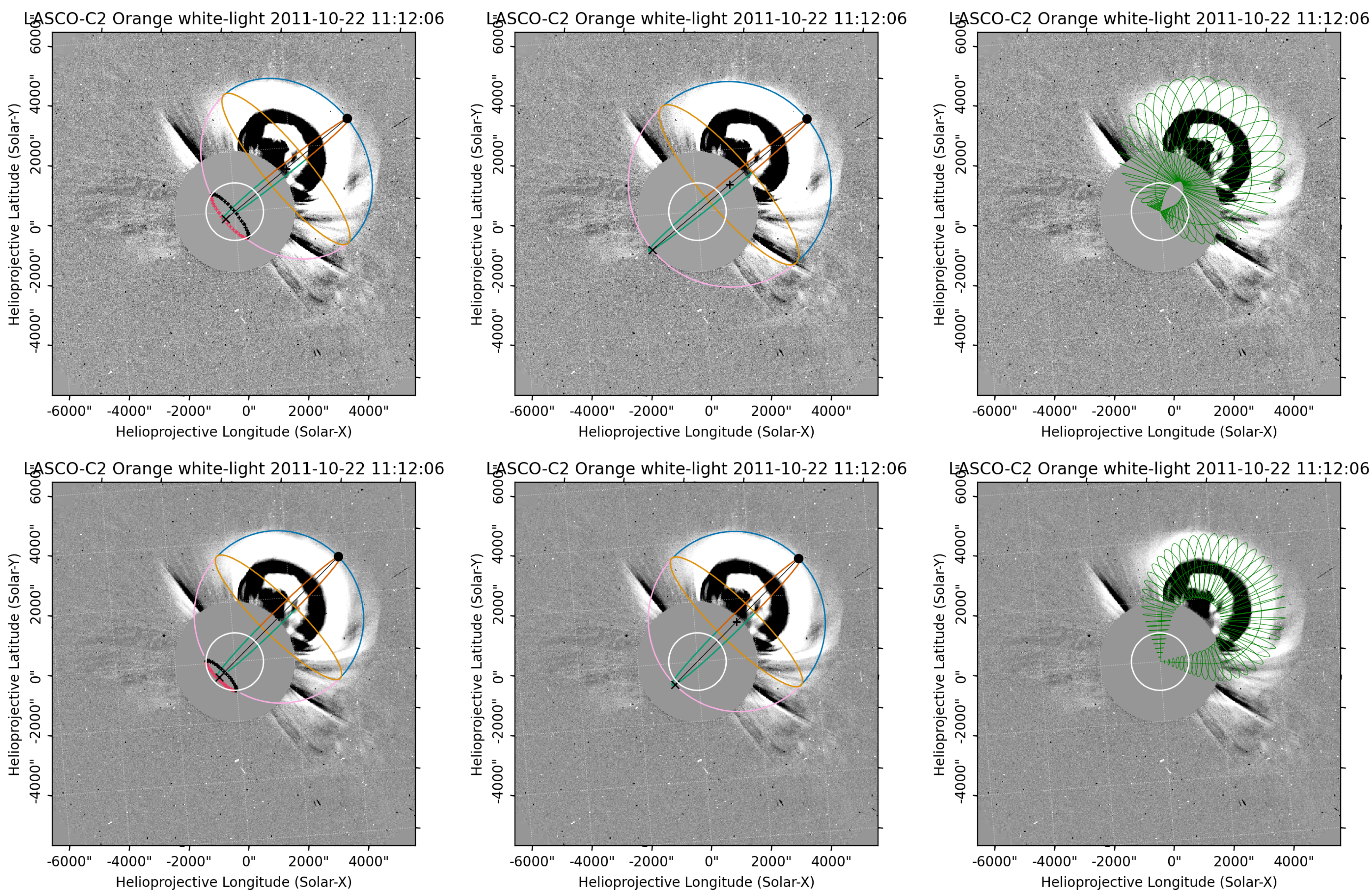
19]. All three models provided by PyThea are applied here: spheroid, ellipsoid and GCS. The fitting is completed by two observers from our team independently and an example of the fits for the event E03 is shown in
Figure 1. Inspecting the fitting results for this example, we see that the reconstructions show a clear bias, as an observer has a subjective ’choice’ of structures to match with the model. Namely, in the top row of
Figure 1 we observe clear shock-related structures (bending of streamers), which the idealized GCS flux rope geometry is fitted on. Hence, the CME width is most probably overestimated. We also find that the overall results, directivity and speed for this event (E03) are less affected by that bias. However, the more complex the choice of structures is, the larger the differences between several observers might be.
For this study we focused on deriving the de-projected CME speeds based on fits completed at two time steps. For each of the three models, the initial CME longitude and latitude was specified by hand. We used the provided locations of the CME-accompanied SFs. We note, however, that these values did not change (substantially or at all) after finalizing the fitting procedure; thus, the final CME directivity provided via PyThea is very crude. Thus, the final CME orientations in the IP space and at Earth are based only on the qualitative information provided by animations from the
http://helioweather.net/archive/ (accessed on 24 February 2023).
4. Discussion
In this study, we present post-event analyses of all GSs observed in SC24 in the search for distinct and reliable GS intensity predictors. The ultimate goal is to derive reliable solar or near-Sun parameters using remote sensing image data that can be applied for early warnings about potential GS onsets and strength. For that, we combined solar, near-Sun and IP parameters, mostly provided by catalogs but also analyzed by us using space-related databases. The results from the novel tool for CME speed de-projection (PyThea) are used for the first time together with the well known parameters in space weather and geophysics research.
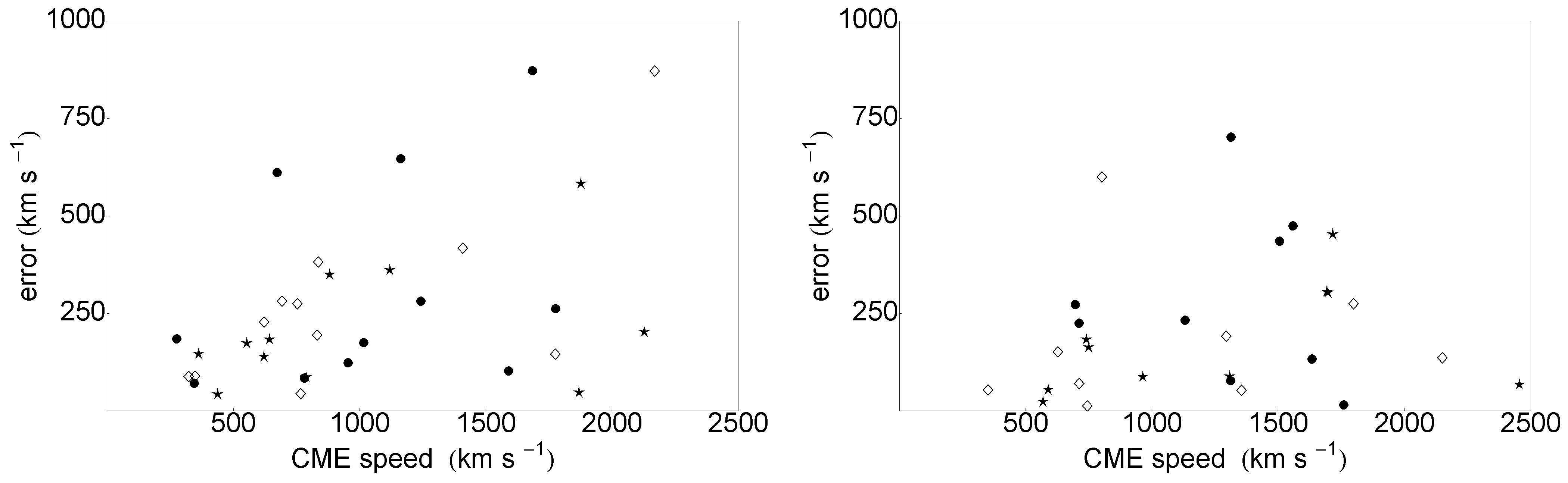
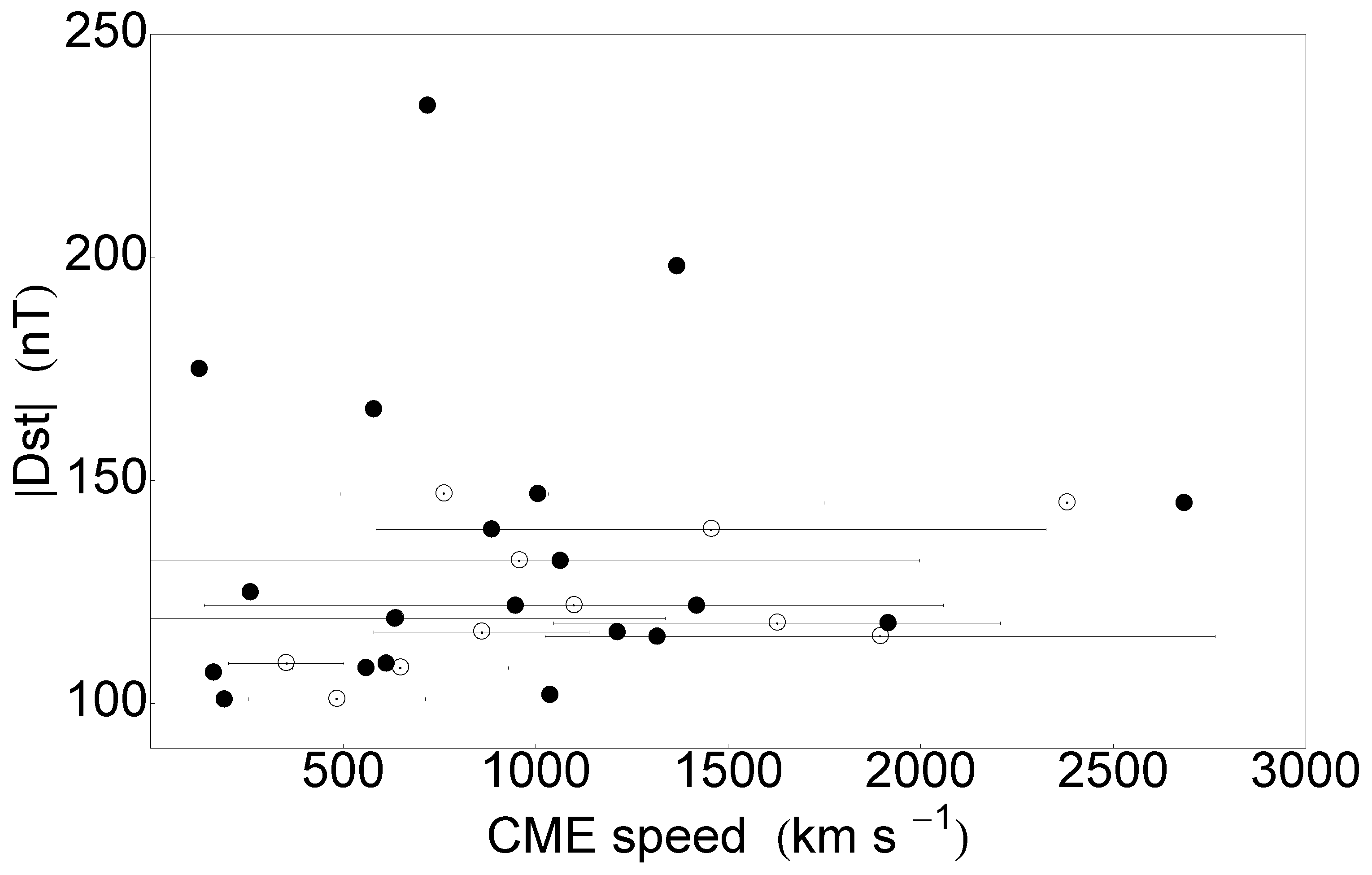
From the considered solar and near-Sun phenomena, selected parameters show a positive correlation with the Dst index. In comparison to the observed projected CME speed, the correlation coefficient could be improved from 0.04 (LASCO) to 0.34–0.55 (using different geometrical models provided via PyThea software package combining LASCO and STEREO data). However, when applying the different CME geometry reconstruction techniques we reveal that especially fast CMEs seem to be prone to large speed errors. Similar results were derived in previous studies that focused on CME arrival time and speed forecasts for Earth, concluding that the CME launch speed might be overestimated for fast events [
44]. This is most probably due to a higher complexity in the ’choice’ of coronal structures that become visible due to the larger compression related to the quickly expanding magnetic structure of the CME. Moreover, for fast halo CMEs large deviations might be found due to the overlap in shock and magnetic structure components strongly affecting the reconstruction quality. For that reason we conclude that the deduced near-Sun 3D parameters continue to have limited forecasting potential for forecasting the GS strength.
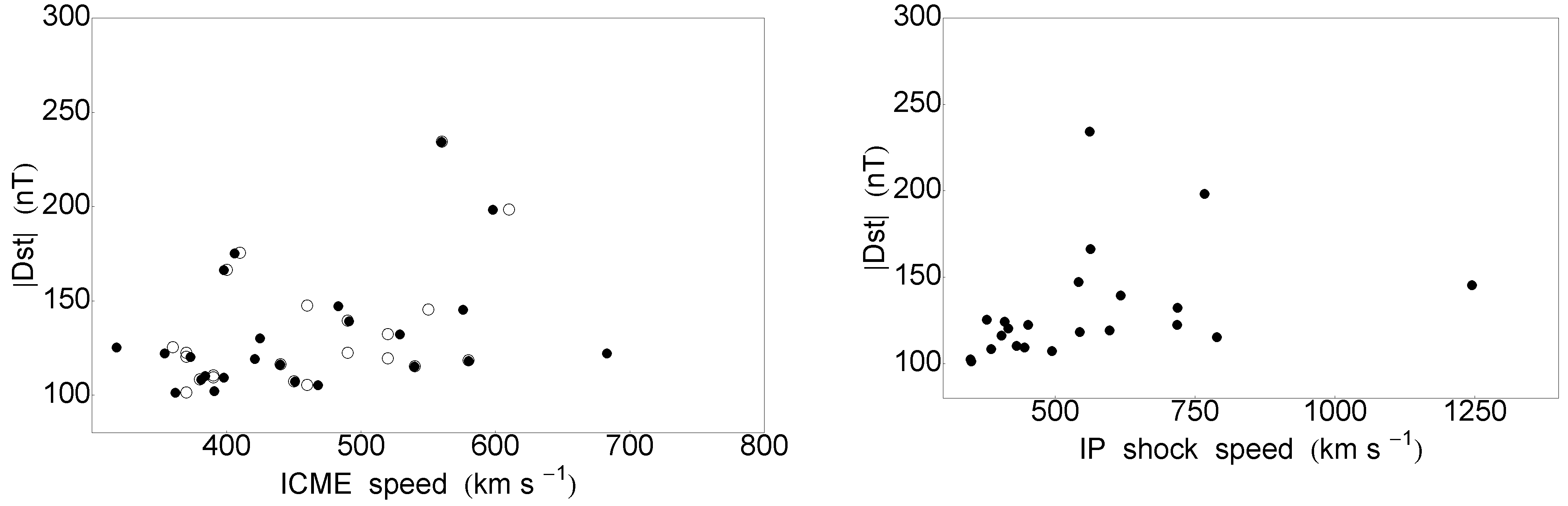
In comparison, most of the selected well known IP parameters deduced from in situ measurements show moderate positive correlations with the GS strength as expected [
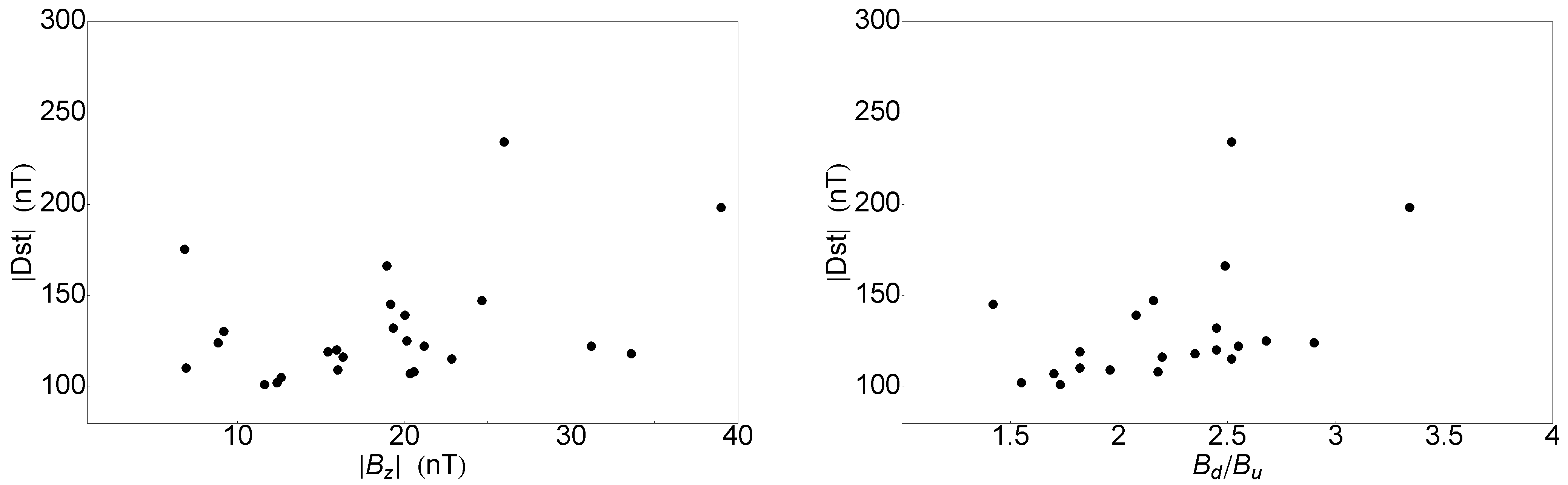
12]. However, for the
parameter (i.e., the southward component of the magnetic field) we find a rather low correlation coefficient of 0.37. This could be due to the limited event sample used here. Other IP parameters, ICME and IP shock speeds, together with their derivative parameters (e.g., Mach number), show a positive trend with the Dst index and correlation coefficients of 0.35–0.45. Therefore, neither of these parameters can be considered as a prevailing one and moreover they are calculated based on single-point in situ observation. Comparing ACE and Wind measurements (see
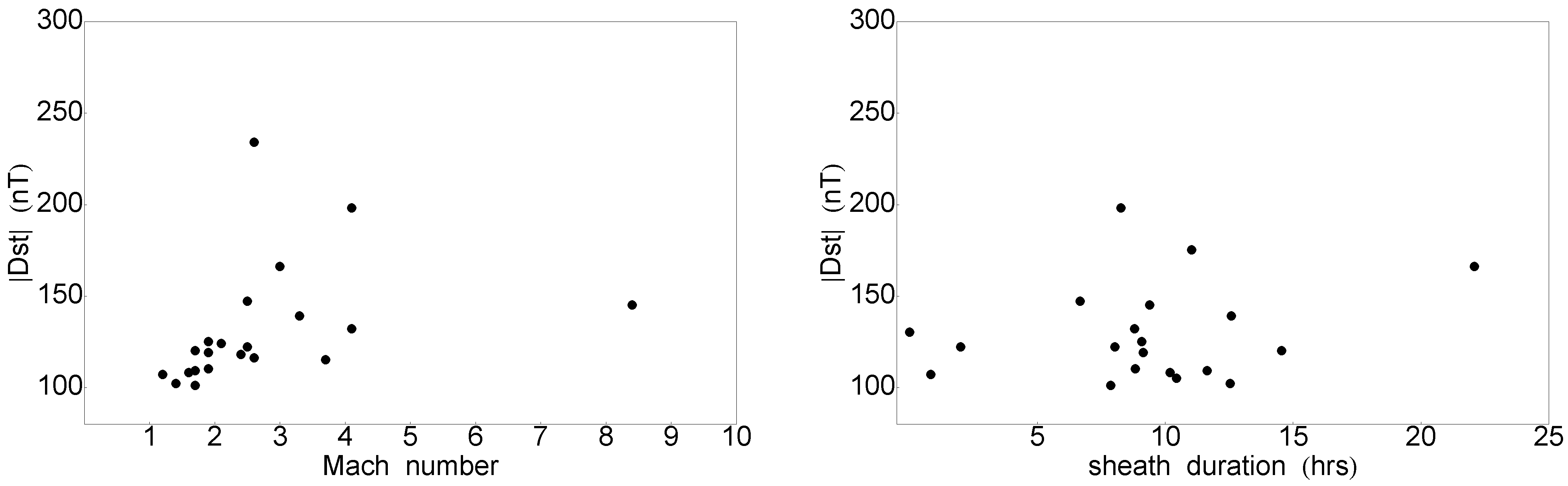
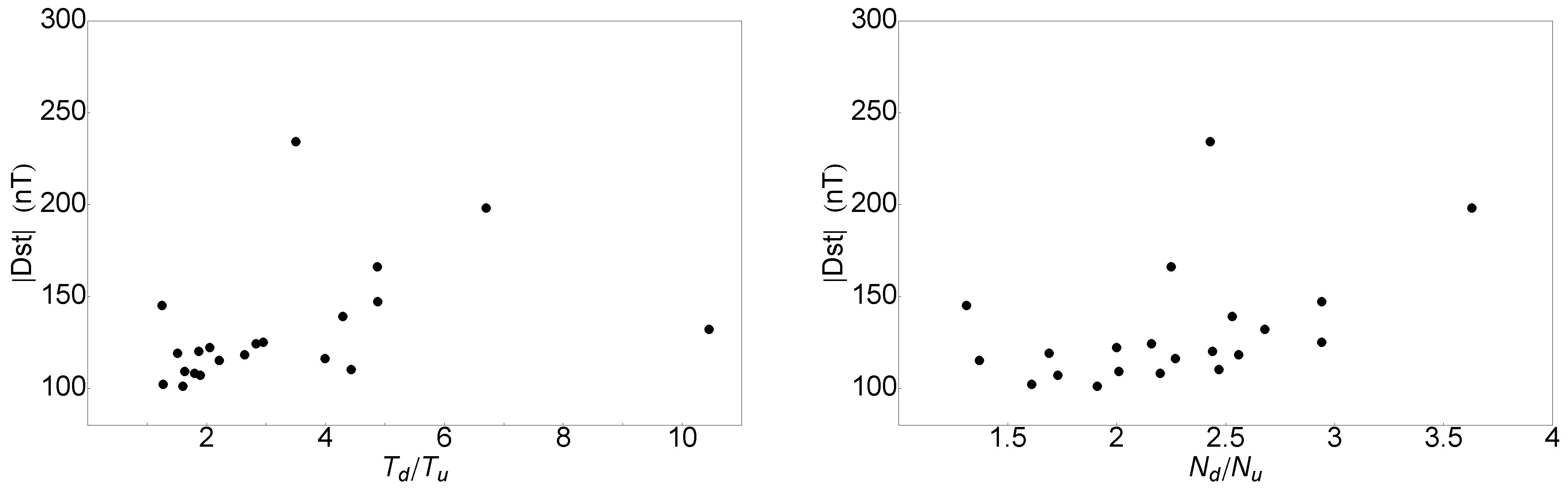
Figure 4) we derive differences in the ICME speed values. Slightly stronger correlation coefficients (0.4–0.5) are obtained when using different shock parameters, e.g., magnetic field, temperature and density jump at the shock profile. In contrast, averaged values of the magnetic field and speed in the magnetic structure, plasma beta in the upstream region or duration of the sheath region show no correlation with the GS strength.
Among all considered solar, near-Sun and IP parameters, only the combination of speed and orientation (nose-like) of the magnetic obstacle seem to have a positive feedback on the GS strength (Dst index), based on the qualitative results provided by
http://helioweather.net/archive/ (accessed on 24 February 2023) animations. As concluded in previous studies, de-projected CME speeds are a necessity for improving the results when modeling CME propagation through the IP space [
45]. However, there seems to be a lack of direct influence of the 3D de-projected CME speed on the GS intensity. Therefore, reliable estimation of the ICME speed distribution over the entire ICME structure upon arrival at Earth seems to be of great importance. Definitely, there is a clear need for permanent stereoscopic observations such as with future ESA Vigil mission that will be positioned at the Lagrange point L5. Future studies should seek a better disentanglement of different CME structures and hence more reliable 3D reconstructions of CME geometries to more reliably estimate the 3D speed and directivity.


