Abstract
The investigation of the magnetic activity of different types of variable stars holds significant implications for our understanding of the physical processes and evolution of stars. This study’s International Variable Star Index (VSX) variable star catalog was cross-matched with Transiting Exoplanet Survey Satellite (TESS) data, resulting in 26,276 labeled targets from 76,187 light curves. A total of 25,327 stellar flare events were detected, including 245 eclipsing binaries, 2324 rotating stars, 111 pulsating stars, and 629 eruptive stars. The results showed that flares from eclipsing binaries, rotating stars, eruptive stars, and pulsating stars have durations such that 90% are less than 2 h, and 91% of their amplitudes are less than 0.3. Flare events mainly occurred in the temperature range of 2000 K to 3000 K. The power-law indices of different types of variable stars were (eclipsing binaries), (rotating stars), (eruptive stars), and (pulsating stars). Among them, the flare energy of pulsating stars is more concentrated in the high-energy range. In all samples, flare energies were distributed from erg to erg. The LAMOST DR9 low-resolution spectral survey has provided H equivalent widths for 398 variable stars. By utilizing these H equivalent widths, we have determined the stellar activity of the variable stars and confirmed a positive correlation between the flare energy and H equivalent width.
1. Introduction
Stellar flares refer to sudden and intense energy release events on the surface of the Sun or other stars, which can be observed as a rapid increase in flux across a broad range of wavelengths. The standard theory states that the reconnection of magnetic field loops in the active outer atmosphere of the star triggers flares, leading to a brief but intense release of energy. During a reconnection event, the magnetic field configuration is altered to a state of lower energy. This often results in the acceleration of high-energy particles towards the star’s atmosphere, leading to the generation of various observable effects across different wavelengths [1,2,3]. Solar flares can be observed with high frequency and rich detail. Therefore, a large part of our comprehension of the flare mechanism and its repercussions is derived from observations of the Sun. Flares on our Sun have energies ranging from to 10 ergs [4]. However, other than the Sun, flares on other stars cannot benefit from the advantage of spatial resolution. Therefore, studies on stellar flares rely on temporal resolution using photometry or spectroscopy. Flares on cooler stars such as K- and M-dwarfs, which are smaller and cooler than the Sun, display properties that differ from the standard solar model. These flares unexpectedly exhibit high energies and, unlike solar flares, show intense continuum or “white-light” emissions, similar to a blackbody at temperatures of 9000–10,000 K superimposed on the stellar spectrum [5,6].
The frequency and energy of flares are correlated with the magnetic field’s strength on the star’s surface. Young, rapidly rotating stars typically have stronger surface magnetic fields and higher flare frequencies, and flare occurrence follows this basic trend [7]. Young T Tauri systems are very active and experience frequent flares [8]. Main sequence stars with low mass or late spectral types (M, K, and G dwarfs) typically exhibit higher flaring rates than their higher-mass counterparts. These low-mass main sequence stars have the potential to experience superflares with energies of up to 10–10 ergs. [9]. The emergence of flares initiates various significant evolutionary processes; this includes the enhanced photoevaporation of protoplanetary disks closer to the star and permanent chemical alterations in the atmospheres of exoplanets. Therefore, flare rates are particularly significant for the early evolution of exoplanetary systems [10]. The maximum flare energy has also been proposed to constrain stellar age [11,12].
Space photometric telescopes and ground-based spectroscopic surveys, such as Kepler/K2 [13], TESS [14], and LAMOST [15,16,17], have been developed significantly. The precision of Kepler is now approaching 10 ppm for bright targets (V = 9–10) and 100 ppm for fainter targets (V = 13–14) [18]; TESS achieves a 1 h photometric precision better than 60 ppm for quiet stars brighter than 7.5 mags and better than 200 ppm for quiet stars brighter than 10 mags [19]. Researchers can now study the stellar activity of different spectral types and ages in more detail. In the search for flares based on Kepler data, 373 flare stars were identified among about 23,000 cool dwarfs [20], as well as flares on A-type stars [21], and 148 G-type superflare stars were found after observing approximately 83,000 stars for 120 days [4]. Through the visual inspection of light curves, Balona [21] detected flares on a broader range of Kepler observations and discovered that even some A-type stars exhibit flare activity. Davenport et al. [22] provided the largest sample of flares for M dwarfs at that time using Kepler data. Davenport [23] discovered about 850,000 flares using four years of Kepler data, covering 4000 stars of spectral types G0–M4, and identified a potential flare saturation threshold based on the Rossby number. Gao et al. [24] searched for flares in binary stars based on Kepler data. It was discovered that the rate of flare occurrence is approximately 10–20% lower in contact and elliptical binaries than in detached and semi-detached systems. Lin et al. [25] estimated the saturation energies for M, K, and G dwarfs to be about 1 × 10 erg, 4 × 10 erg, and 1 × 10 erg, respectively, and also estimated the power-law index for the flare frequency distribution for these three spectral types to be 1.82 ± 0.02 (M dwarfs), 1.86 ± 0.02 (K dwarfs), and 2.09 ± 0.04 (G dwarfs).
Günther et al. [26] examined flares in 24,809 stars observed during the initial two months of the TESS mission and observed that the energy of flares varied from 10 to 10 erg. It was confirmed that fast-rotating M-type dwarf stars were the most prone to flaring and that the amplitude of the flares was not dependent on their rotation period. The team detected 8700 flare events in 1228 stars, with the highest flares occurring in M4.5 and higher dwarf stars. By examining the K2 data of Pleiades, Praesepe, and M67, Ilin et al. [27] detected and examined flares, concluding that flare activity diminishes over time. This decline was more pronounced in stars with higher effective temperatures (). A convolutional neural network (CNN) was employed by Feinstein et al. [28] to scan for flares. Their research revealed that low-mass stars ( < 4000 K) exhibit higher flare rates and energies at all stages of their evolution. In contrast, hotter stars demonstrate increased flare rates and amplitudes. Yang et al. [29] searched for flare events in the targets of sectors 1–30 of TESS and found over 60,000 flare events; they also found that eclipsing binary stars exhibit a higher frequency of flares compared to single stars.
The magnetic field is the most critical factor in stellar activity, as Parker [30] and other researchers demonstrated. Clues left by stellar activity can be found in the corona, chromosphere, and photosphere, which can be established on the emission of H and Ca II lines and coronal X-rays. Previous studies have shown that stellar activity is closely related to rotation period and convective depth [31,32,33]. Yi et al. [34] investigated the magnetic activity characteristics of 58,360 M dwarf stars in the LAMOST survey using H emission lines as a basis. By combining data from LAMOST and Kepler, Chang et al. [35] analyzed the magnetic activity of 54 M dwarf stars and determined that M dwarf stars with more strong H emission levels generally experience more massive flares. Utilizing the extensive photometric data provided by Kepler, Yang et al. [36] identified 540 M dwarf stars and cross-matched them with LAMOST DR4 to obtain spectra for 89 M dwarf stars that had exhibited flares. Lu et al. [37] found that the correlation between chromospheric activity and flares was analyzed by merging spectra from LAMOST DR5 with light curves from the Kepler and K2 missions, obtaining a spectra catalog for 516,688 M-type stars. We hope to investigate the magnetic activity characteristics of flare stars and their correlation with various parameters. We are particularly interested in the connection between chromospheric activity and flares, as it is one of the most prominent manifestations of magnetic activity. By utilizing the spectral data from LAMOST DR9, we can obtain more accurate and detailed information on chromospheric activity and further explore the relationship between flares and magnetic activity.
We searched for flare events in TESS and VSX [38] cross-matched data. We obtained flare parameters for different types of variable stars and performed statistical analysis on the flare characteristics of these four types of variables. Section 2 presents the data used in our analysis. Section 3 describes our method for identifying flare events, presents our flare search results, and discusses the flare characteristics of eclipsing binary, rotating, eruptive, and pulsating stars. Section 4 of the paper focuses on the magnetic activity of flare stars and involves an analysis of the low-resolution spectra obtained from LAMOST. In Section 5, we summarize the existing research work.
2. Data
2.1. TESS Data
The Transiting Exoplanet Survey Satellite (TESS) [39] was launched by SpaceX Falcon, a space telescope within NASA’s Explorer program, on 18 April 2018. Its primary objective is to investigate the presence of planets around stars within a 300-light-year vicinity of Earth. TESS’s mission is divided into several phases: the first year (July 2018–July 2019) focused on observing the southern ecliptic hemisphere; the second year (July 2019–July 2020) was dedicated to the northern hemisphere; the third year (July 2020–July 2021) entailed re-observation of the southern hemisphere; the fourth year (July 2021–September 2022) involved re-observation of select northern hemisphere regions and the first observation of a 240-degree ecliptic belt, encompassing 16 sectors. In the fifth year, TESS aimed to complete the northern hemisphere survey and initiate a new southern hemisphere investigation. In the initial two years of its mission, TESS conducted high-precision photometry on approximately 200,000 stars at roughly two-minute intervals, covering nearly the entire sky through 26 sectors, each spanning 24 degrees by 96 degrees, with each sector observed for 27.4 days. Commencing in the third year, TESS initiated an extended mission with a similar data collection cadence for approximately 20,000 targets per sector. Additionally, a 20 s data collection mode was introduced, enabling the observation of up to 1000 targets per sector. TESS’s light curve data are processed through the TESS pipeline, an improvement on the pipeline utilized during the Kepler mission [40,41,42]. Each target pixel file (TP) undergoes data reduction using the simple aperture photometry (SAP) method, with the light curves of all targets stored in a flux array. Subsequently, the data are detrended using contrending basis vectors, and the processed light curves are stored in another array, referred to as pre-search data conditioning (PDCSAP). In this study, by cross-matching the International Variable Star Index (hereafter VSX) [38] with the TESS sectors S1–S56, we obtained 76,187 light curves for 26,276 targets. We then searched for flare events on this dataset.
2.2. LAMOST Spectra
The Guoshoujing Telescope, also known as the Large Sky Area Multi-Object Fiber Spectroscopic Telescope (LAMOST), is a major national infrastructure of the National Astronomical Observatories, Chinese Academy of Sciences, located at the Xinglong Observatory base in Hebei Province, China [15]. With an equivalent aperture of 4 m and a field of view of 5 degrees, LAMOST can observe more than half of the sky, covering a spectral range of 370 nm–900 nm. To achieve multi-object fiber spectroscopy, 4000 optical fibers were arranged at the focal plane [16,17]. On 31 March 2022, the LAMOST Data Release 9 (DR9) was officially released, which includes the pilot survey and the first nine years of the formal survey data. DR9 v1.0 contains 5533 low-resolution observation fields and 1529 medium-resolution observation fields. The total number of spectra reaches 19.44 million, including 11.22 million low-resolution spectra, 1.84 million non-time-domain medium-resolution spectra, and 6.38 million time-domain medium-resolution spectra. In addition, DR9 also includes a stellar spectroscopic parameter catalog of approximately 8.79 million stars.
We cross-matched the LAMOST DR9 dataset with 3174 stars exhibiting outbursts and excluded samples with a signal-to-noise ratio (S/N) of less than 10. After the selection, we obtained 1108 low-resolution spectra from 398 stars. In this study, we utilized the H equivalent width provided by the low-resolution spectra to assess the activity of variable stars. We analyzed the correlation between outburst energy and equivalent width.
3. Flare Detection
3.1. Searching for TESS Flare
Flares are defined as powerful eruptions on a star’s surface that often involve high-energy radiation emission. Flares typically arise near active regions of the magnetic field on the star due to the discharge of magnetic field energy. The brightness of these eruptions exhibits a noticeable increase in both visible light and ultraviolet wavelength bands, with some even showing significantly enhanced radiation in the X-ray and gamma-ray bands [43,44]. Various methods exist for searching for flares, with one common approach being based on time-series analysis. This method often involves utilizing change-point detection techniques, such as scanning the time series for dramatic brightness fluctuations [20,22,23,24,25,26,36,37,45,46,47,48,49,50]. Moreover, some algorithms employ convolutional neural networks to detect flares automatically Feinstein et al. [28]. Webb et al. [51] proposed an unsupervised approach to detect transients by employing clustering techniques and the ASTRONOMALY package [52], which allows for rapid flare identification and further analysis. Vida and Roettenbacher [53] employed the RANSAC (RANdom SAmple Consensus) algorithm to search for flares, demonstrating performance on par with manual inspection in the Kepler dataset. In this study, we applied a method similar to Su et al. [54] and Yang et al. [29] for flare detection in 76,187 light curves. First, we normalized the data as follows:
In this equation, represents the normalized flux, denotes the PDCSAP flux value for each TESS target, and is the median of the PDCSAP flux.
After obtaining the normalized data, we used multiple fitting tests to find the most suitable segmentation length to divide the TESS 27 day data. We subtracted the mean value from the abscissa of each light curve to center them around zero. Each segment of the segmented light curve has a 60% overlap with the neighboring segments. This was performed to facilitate subsequent analysis and processing and to avoid the Runge phenomenon caused by polynomial fitting. Afterward, we used polynomial fitting to find the background light curve for each data segment. To determine the optimal polynomial fit, we incrementally increased the polynomial order until increasing the order no longer significantly reduced the fitting residuals. At this point, the most suitable fitting function had been found. This fitting process was repeated ten times, with data points exceeding three times the standard deviation removed during each iteration. Then, we refitted the remaining data, obtaining the background light data and its proper function after ten iterations. After normalization and background fitting, we identified the relevant data points. Initially, we eliminated the background light curve from the original light curve and then identified all occurrences that surpassed four times the standard deviation. We then visually inspected these points for the characteristics of rapid increases and slow declines and excluded potential contamination sources. Finally, we confirmed the flare events. To ascertain the start and end times, we defined the start of a flare event as when the brightness first surpasses 5% of its peak value. The brightness then starts to decline until it returns to the baseline level; we define the end of a flare event as when the brightness drops below 5% of its peak value. To determine the magnitude of a flare, we subtracted the fitted function of the background light curve at the corresponding time from the highest recorded value of the flare. Figure 1a–d shows examples of flare event searches for eclipsing binary, rotating, eruptive, and pulsating stars, respectively. For the eclipsing binary example shown in Panel a, we performed a background fitting using polynomials, increasing the polynomial order to find the best fit. When the polynomial order exceeded three, the residual did not decrease significantly, indicating that third-order polynomials are the best-fitting function. We repeated the data fitting at the top of the panel ten times, removing points greater than three times the standard deviation and marking these points as green, as shown at the top of Figure 1a. The middle of Figure 1a shows the background we obtained after removing the green points, with the red line representing our fitting function. Subtracting the background from the original light curve, we obtained the bottom panel of Figure 1a, with points greater than four times the standard deviation marked in red. In subsequent visual inspections, we determined that Figure 1a met the criteria for a flare event and is thus a flare event.
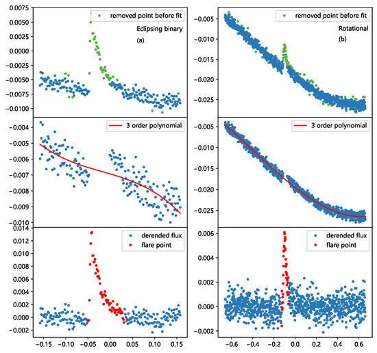
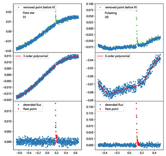
Figure 1.
Exploring flare event phenomena: (a) eclipsing binaries, (b) rotating stars, (c) eruptive stars, and (d) pulsating stars The top panel of Figure (a) shows the observational data, where the green dots correspond to the data points removed during the fitting process. In the middle panel, we fit the background with a sixth-order polynomial and subtracted it from the raw light curve, resulting in the flares shown in the bottom panel.
In Figure 2, we show the smaller flares we have discovered, with the smallest amplitude being about 0.001 and the shortest duration being about 14 min. These amplitudes and durations represent the lower limits of the flares we have found. The discovery of these flares benefited from the advantages of the TESS telescope in studying flares. Tu et al. [55] and Yang et al. [29] searched for flares using TESS data, and the durations of the flares they found were mainly concentrated around 1 h. The amplitudes were also usually small, with a minimum of about 0.001, consistent with our search range. TESS has strong capabilities in finding smaller flares because the targets observed by TESS have a high signal-to-noise ratio. Based on TESS’s 2-min sampling rate, the properties of flares, including their duration and energy, can be obtained more accurately. In addition, the TIC provides rich stellar parameters, which also help study flares.
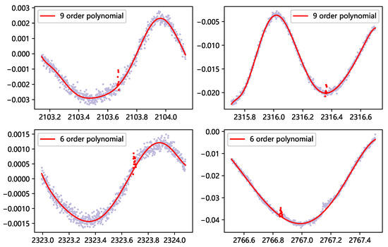
Figure 2.
Examples of four smaller flares identified in the TESS survey.
3.2. TESS Flare Energies
We identified 25,327 flares from 3174 stars in the 76,187 light curves of 26,276 targets. Utilizing the classification provided by the VSX, our sample of flare stars includes 245 eclipsing binaries, 2324 rotating stars, 629 eruptive variables, and 111 pulsating variables. The same star may have multiple variability type labels, and it may be classified into different categories simultaneously. However, the number of such stars is small, and their influence on the overall classification is limited. The left panel of Figure 3 depicts the proportion of variable stars with flares in the overall sample, with blue indicating the total number and red indicating the number of stars with flare events. Notably, the highest proportion of flare events is found in rotational and eruptive variables, reaching 30% and 38%, respectively, while the proportions for eclipsing binaries and pulsating variables are only 4% and 2%, respectively. The right panel presents the average flares and the total flare events for each variable type. The average number of flares in rotational and eruptive variables is higher than in eclipsing binaries and pulsating variables, leading to a significantly lower number of flare events in the latter two categories.
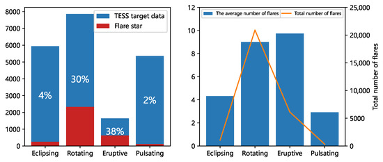
Figure 3.
Proportions of variable stars with flares for different types (left) and total and average numbers of flare events for different types (right).
To classify the evolutionary stages of our target variable stars, we used the method of Notsu et al. [56] and plotted different types of eruptive variables in Figure 4. The background of these plots is based on the distribution of main sequence stars, subgiant stars, and red giant stars provided by Berger et al. [57] using Kepler data. In Subplot a, we classified 216 eclipsing binaries with flares, of which 148 (69%) were categorized as main sequence stars, 57 (26%) were categorized as subgiant stars, and the remaining 11 (5%) were categorized as red giant stars. Subplot b contains 2098 rotational variables, of which 1912 (91%) are main sequence stars, 129 (6%) are subgiant stars, and 57 (3%) are red giant stars. In Panel c, we classified 550 eruptive variables, of which 520 (94%) are main sequence stars, 20 (3%) are subgiant stars, and 10 (2%) are red giant stars. Finally, in Panel d, we classified 75 pulsating variables, of which 41 (54%) are main sequence stars, 2 (3%) are subgiant stars, and 32 (43%) are red giant stars. In general, most of them are main sequence stars, with a small portion being subgiant and red giant stars. Flares are an indicator of stellar activity level, and the distribution and evolution of flaring stars are related to those of stars. In Figure 4, most of our flaring variables are concentrated on the right. Yang and Liu [58] plotted the distribution of 3420 flaring stars on the H-R diagram and found that these objects are mainly distributed in the late-type region. They also indicated that a few giant stars exhibit active flaring activity, but most are relatively inactive, which is consistent with the dynamo theory and magnetic observation results.
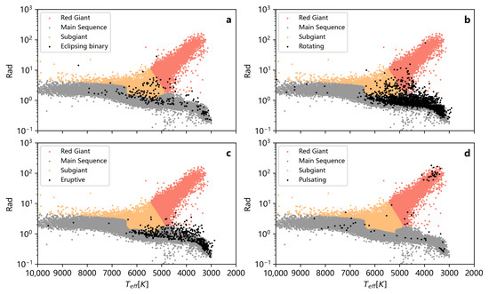
Figure 4.
The distribution of the radius (R) and effective temperature of stars of different types are shown in the figure. The background colors are based on the marking of all 177,911 Kepler stars listed by Berger Berger et al. [57], where red represents red giants, orange represents subgiants, and gray represents main sequence stars. In the figure, we use black to represent variable stars with eruptive phenomena, where (a–d), respectively, represent the distribution of eclipsing binary, rotating, eruptive, and pulsating stars.
The energy of these flares was calculated using the following equation:
Here, represents the flare energy, denotes the stellar radius, is the Stefan–Boltzmann constant, signifies the star’s effective temperature, and is the normalized PDCSAP flux. The effective temperature and stellar radius were derived from the TESS Input Catalog (TIC) [59], which is based on the GAIA DR2 catalog and incorporates a variety of other catalogs [60], including the Two Micron All-Sky Survey (2MASS), the Fourth US Naval Observatory CCD Astrograph Catalog (UCAC4), the AAVSO Photometric All-Sky Survey (APASS), the Sloan Digital Sky Survey (SDSS), and the Wide-field Infrared Survey Explorer (WISE) [61,62,63,64]. Due to the absence of radius or effective temperature information for specific targets, we were able to determine the energy of 21,989 flare events from 2783 stars. In Table 1, we present a comprehensive overview of pertinent parameters for the flaring stars under investigation, encompassing the initiation and termination times of flares, the associated energy release, and the variability period reported in the VSX catalog and the respective stellar classification. Following the General Catalogue of Variable Stars (GCVS) [65] classification scheme, we have meticulously detected 1060 flaring instances within 245 eclipsing binary systems, with 20,908 flares among 2324 rotating stars, 324 flaring events in a sample of 111 pulsating variables, and 6127 flare occurrences across 629 eruptive stellar objects, thereby offering a comprehensive perspective on distinct variable star categories.

Table 1.
Flare parameters of TESS variable stars.
As illustrated in Figure 5, the flare energy distribution of our data spans a range from 3.99 × 10 erg to 6.18 × 10 erg. Previously, Tu et al. [55,66] searched for superflares in solar-type stars captured during the initial and subsequent years of the TESS mission. This resulted in the detection of 2988 superflares from 711 solar-type stars, with maximum flare energies of 1.24 × 10 erg and 1.77 × 10 erg in the first and second years, respectively. Su et al. [54] investigated flare events in the initial 24 sectors of TESS data, with flare energy ranging from 4.25 × 10 erg to 3.23 × 10 erg. Our obtained energy distribution aligns with previous findings, with the most considerable flare energy in our study reaching erg, surpassing the erg reported by Tu et al. [55]. We have identified only six stars with flare energies exceeding erg, namely TIC 220424200, TIC 117655534, TIC 445271527, TIC 320321218, TIC 7620704, and TIC 20319183. These objects are giants with radii measuring 113.408, 154.247, 83.868, 79.174, 91.515, and 90.34 times the solar radius, respectively, which accounts for the maximum flare energy exceeding erg. The flare energy of the entire sample shows a concentrated distribution centered around erg, with a gradual decrease in proportion on both sides. The flare event energies of rotating stars and eruptive variables correspond to the overall distribution. For eclipsing binaries, a higher proportion of lower-energy flare events, specifically those with energies around erg, is observed. In pulsating variables, superflares with energies greater than erg constitute the highest proportion, reaching 43%, while the proportions for eclipsing binaries, eruptive variables, and rotating stars are 22%, 13%, and 13%, respectively.
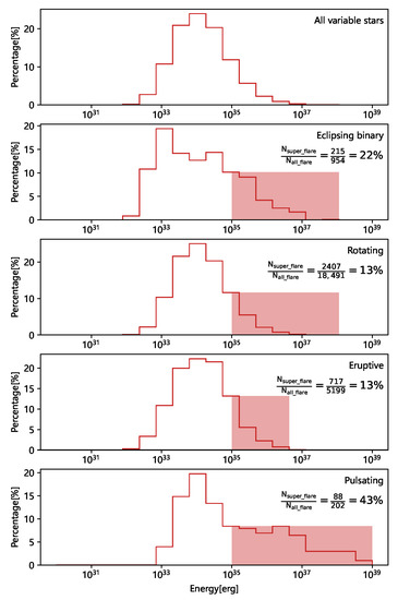
Figure 5.
Energy distribution of flares in different types of variable stars. The red portion represents flares with energy greater than ergs. represents the number of events in the current type of variable star with energy greater than ergs, and represents the total number of flares in the current type of variable star.
3.3. Flare Duration and Amplitude
We conducted a detailed statistical analysis of the duration and amplitude distribution for eclipsing binaries, rotating variables, eruptive stars, and pulsating variables. We found that the duration of flares for each type of variable star is concentrated within 2 h (see Figure 6). According to our statistics, the proportion of flare events within 2 h is 93%, 90%, 90%, and 90% for the respective categories. We conducted KS tests on the duration of flares in four types of variable stars. The results showed that the p-value for comparing eclipsing binaries and pulsating variables was 0.19. The p-values for the comparisons between eclipsing binaries and eruptive variables and between eclipsing binaries and rotating variables were both less than the significance level of 0.01. Moreover, the p-values for comparing eruptive and rotating variables, eruptive and pulsating variables, and rotating and pulsating variables were 0.047, 0.069, and 0.077, respectively. These findings indicate that different types of variable stars share similar features in the duration of flares. Recently, Lin et al. [25] investigated flares in G, M, and K dwarf stars and found their durations concentrated around 1.5 h, with the longest flares reaching approximately 5 h. Walkowicz et al. [20] observed flare durations of 3–5 h in their Kepler survey. Yang et al. [29] conducted a large-scale flare event analysis using TESS data and discovered that over 90% of the events were shorter than 2 h. Furthermore, flare amplitudes exhibit similar characteristics, mainly ranging between 0.01 and 0.1. We investigated the amplitude distribution of different types of variable stars and found that 75% of amplitudes were less than 0.1, while over 91% were less than 0.3. These findings indicate that flare duration and amplitude are focused in a relatively narrow range. Günther et al. [26], Yang et al. [29], Tu et al. [55] identified a concentration of flare amplitude in the range of 0.001–0.1 from TESS data. Our findings are consistent with the existing literature.
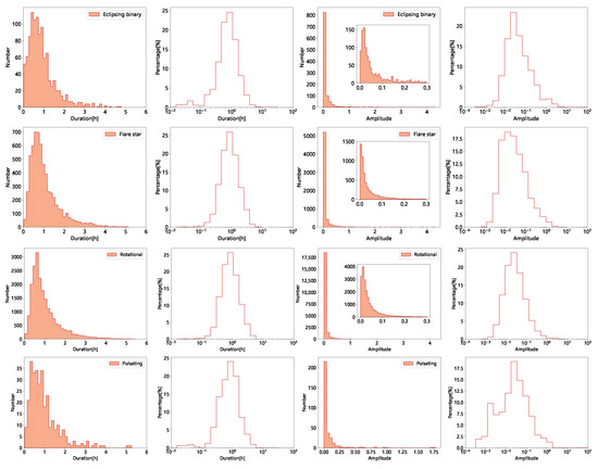
Figure 6.
The distribution of flare durations, including the number and percentage, for different types of variable stars is presented, along with the distribution of flare amplitudes in terms of both the number and percentage.
Lin et al. [25] identified power-law relationships between the amplitude and the effective temperature () of the star () and between the amplitude and the mass of the star (), revealing an inverse correlation between the amplitude of flares and the temperature/mass of the star. We performed a regression analysis to investigate the relationship between the amplitude of flares and stellar parameters, as shown in Figure 7. The analysis yielded power-law relationships of and , which confirmed the presence of a negative correlation between flare amplitude and stellar parameters. The values for the relationship between amplitude and temperature for different types are as follows: , , , and . The values for amplitude and mass are , , , and . Figure 8 also displays the relationship between flare energy, temperature, and mass for variable stars, all of which exhibit positive correlations with flare energy.
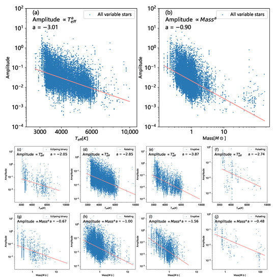
Figure 7.
(a,b) depict the relationship between the amplitude of all flare events and stellar parameters. At the same time, (c–f) illustrate the correlations between amplitude and temperature for distinct variable star types. Additionally, (g–j) illustrate the relationship between amplitude and mass for various variable stars.
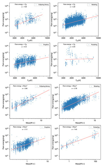
Figure 8.
Illustration of a positive correlation between flare energy and stellar parameters for different types of variable stars.
3.4. Flare Occurrence Percentages
The occurrence frequency represents the proportion of total flare duration for a given star relative to its total observation time. The percentage of flares can be calculated using the equation given by Walkowicz et al. [20], as shown in Formula (3).
Here, denotes the complete duration of flares for each star, and represents the total observation duration for each star.
Figure 9 illustrates the percentage distribution of flares for various stellar types. The flare percentage in our sample increases within the 0–2% range and then gradually declines, with 95% of variable stars having a flare occurrence rate within 5%. The highest number of stars exhibit a flare occurrence rate between 1% and 2%. In the study by Yang et al. [29], out of 1,347,800 flare stars, 12,763 exhibit a flare rate between 0% and 1%. Several studies have also verified that there is an increase in the percentage of flares that occurs as the effective temperature decreases [25]. For different types of variable stars, Yang et al. [29] found that eclipsing binaries are more prone to flares than single stars. Huang et al. [48] observed a significantly higher flare frequency in eclipsing binary stars than individual M dwarfs. We found that the flare occurrence rate for eclipsing binaries and pulsating variables is mainly concentrated between 0 and 1%, while rotating and eruptive variables are mainly concentrated between 1–2%, indicating that rotating and eruptive variable stars have a higher flare frequency than eclipsing binaries and pulsating variables.
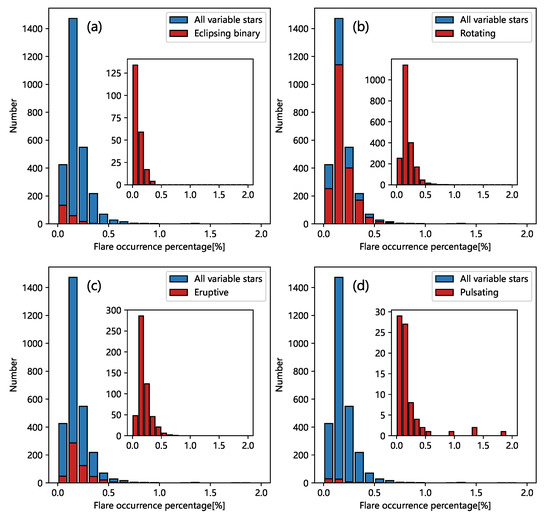
Figure 9.
Panels (a–d) represent the distribution of flare percentages for eclipsing binary, rotating, eruptive, and pulsating stars, respectively. Rotating and eruptive-type stars tend to exhibit higher flare percentages.
3.5. Ratio of Flaring Stars to Total Stars
Figure 10 demonstrates the distribution of flare occurrences for various variable stars in the temperature range of 2000 K to 10,000 K. As the temperature rises, the fraction of variable stars displaying flares decreases, with flare events primarily occurring on stars between 2000 K and 3000 K. Among these stars, 38.5% exhibit flaring phenomena, a percentage higher than the 24% reported by Yang et al. [29] for the 2500 K–3000 K range. Walkowicz et al. [20] and Lin et al. [25] found that stars with lower temperatures have a higher probability of flaring than those with higher temperatures, which our study corroborates. In terms of temperature range, we find that variable star flares are concentrated between 2000 K and 6000 K, higher than the range of up to 4000 K reported by Günther et al. [26] and Jackman et al. [67]. Yang et al. [29] revealed that eclipsing binary stars are more susceptible to flaring than single stars, particularly at temperatures below 6000 K. Huang et al. [48] posited that magnetic interactions between the two stars in binary systems make eclipsing binaries more flare-prone than M dwarfs. We observe that the flare proportion of eclipsing binaries gradually decreases as the temperature increases, peaking at 24.1% within the 3000 K–4000 K range. Within this temperature range, rotating stars are relatively less likely to experience flare events, while eruptive and pulsating stars are more common, with 53.8% and 33.1% flare proportions, respectively. Within the 3000 K–6000 K range, the flare proportion of eruptive stars increases as the temperature rises. In the 4000 K–5000 K range, rotating and pulsating stars are more likely to produce flare events.
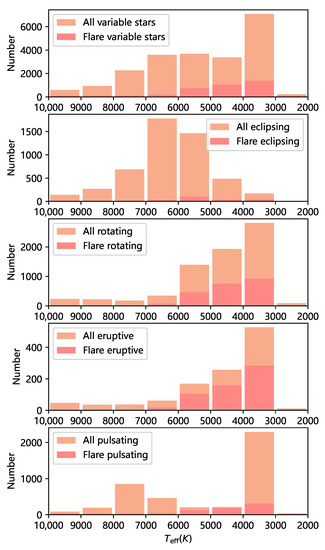
Figure 10.
Distribution of different types of variable stars within the 2000 K–10,000 K range.
3.6. Duration, Amplitude, and Energy
Figure 11 depicts the correlation between flare energy and duration for various categories of stars. We refer to the power-law relationship between energy and time as , defined as the relationship between energy (E) and duration (D): . This implies that as the duration increases, the energy correspondingly escalates. The steeper the power-law relationship, the more rapidly the energy increases, resulting in larger energy values for extended durations. Recent studies by Yang et al. [29] demonstrated that , with values for A-, F-, G-, K-, and M-type stars being , , , , and , respectively. Our overall sample has a value of 0.23, which is consistent with the aforementioned result. Panel (c) displays the relationship between flare energy and duration for eclipsing binaries. Eclipsing binary systems consist of two closely connected stars whose orbits cause them to obscure each other, leading to changes in brightness periodically. Our study reveals that the power-law relationship index for flare energy and duration in eclipsing binaries is 0.13, indicating a relatively weaker relationship with a minor impact of increasing duration on energy. For eruptive variables (Panel e), the changes in brightness are attributed to intense processes and flares occurring in the chromosphere and corona. Our research finds that the power-law relationship index for flare energy and duration in eruptive variables is 0.27, steeper than that of eclipsing binaries. This suggests a more pronounced relationship between flare energy and duration in eruptive variables, with a more significant impact of increasing duration on energy. We observe that the relationship between flare energy and duration for rotating variables (Panel d) exhibits a power-law distribution with a power-law index of 0.26, similar to eruptive variables. However, we did not detect a notable power-law correlation between flare energy and duration in pulsating variable stars (Panel f), which may be due to the smaller number of pulsating variables. Our findings, illustrated in Figure 11, show the relationship between flare amplitude and energy as described by the formula . We found that for eruptive and rotational variables, the value of a was 0.29 and 0.39, respectively, which is consistent with the overall sample trend of 0.26. However, no clear pattern emerged for eclipsing binaries, with a value of . As for pulsating variables, we found a value of , contrary to the overall trend, suggesting that flare energy decreases as amplitude increases. For panels f and g, there may be fitting biases due to the limited sample size. Additionally, since the sample size of pulsating variables is limited, we need to expand the sample size further to investigate this phenomenon more deeply.
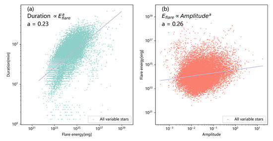
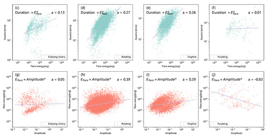
Figure 11.
The relationship between flare energy and duration for different types of stars is depicted as follows: Panel (a) displays the entire sample; Panel (c) showcases eclipsing binaries; Panel (d) features rotating variables; Panel (e) presents eruptive stars; and Panel (f) illustrates pulsating variables. The relationship between flare energy and amplitude for diverse categories of stars is illustrated as follows: Panel (b) exhibits the entire sample; Panel (g) highlights eclipsing binaries; Panel (h) focuses on rotating variables; Panel (i) demonstrates eruptive stars; and Panel (j) reveals pulsating variables.
3.7. TESS Flare Frequency Distribution
The flare frequency distribution (FFD) is a commonly employed method to describe the correlation between the frequency of stellar flare occurrences and their energy. We utilized the maximum likelihood estimation approach to compute and evaluate the distribution of flare frequencies [68,69,70,71], as shown in Equation (4); we used Equation (5) to compute the error:
In these equations, represents the frequency distribution slope, n denotes the number of flares, and denote the highest and lowest values in the flare dataset, and is the error. We calculated the overall flare frequency distribution and the flare frequencies for eclipsing binaries, rotational variables, eruptive variables, and pulsating variables. The distribution of flare energies conforms to a power law solely at higher energy levels [72], and different researchers have adopted varying energy ranges to analyze the power-law distribution of stellar flares. For instance, Yang et al. [36] considered a range of erg and above, Su et al. [54] selected flares with energies above erg, Wu et al. [46] employed a range of – erg, while Maehara et al. [4] and Shibayama et al. [73] used a range of – erg. Given that the quantity of flare occurrences in our sample is limited to below erg and above erg, we chose an energy range of erg– erg to calculate the overall distribution. We chose the same energy range as the overall sample for rotational and eruptive variables. For eclipsing binaries, we selected the erg– erg energy range, as many flare events also occur within this range. For pulsating variable samples, we selected an energy range of erg– erg.
Figure 12 top shows the flare frequency distribution of all variables in different effective temperature ranges. The exponent value is . We calculated the values for flare events in different temperature ranges: 2000–3500 K, 3500–5000 K, 5000–6000 K, and 6000–7500 K. The values for flares in these temperature ranges are , , , and , respectively. This implies that the flare frequency distribution and energy relationship differ across temperature ranges, with the index increasing and gradually decreasing as the temperature rises. Tu et al. [55,66] obtained values of and from TESS 1–13 and 13–26 sector observations, respectively, while Su et al. [54] reported an of . They also provided values for flares at 2000–3500 K, 3500–5000 K, and 5000–6000 K, which were , , and , respectively. For eclipsing binaries, rotational variables, eruptive variables, and pulsating variables, their power-law relationship indices are , , , and , respectively. Furthermore, we calculated the values for eclipsing binaries at temperature ranges of 2000–3500 K, 3500–5000 K, 5000–6000 K, and 6000–7500 K, which were , , , and , respectively; for rotational variables, they were , , , and ; for eruptive variables, they were , , , and . Due to the small sample size of pulsating variables, we could not calculate their frequency distribution by temperature. We found that eclipsing binaries and pulsating variables generally had smaller values, while rotational and eruptive variables had larger values. This suggests significant differences in the flare frequency distribution and energy relationship between different variable star types, necessitating more advanced research for each specific variable star type.
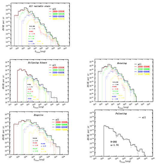
Figure 12.
The flare frequency distributions of all flare stars, eclipsing binaries, rotational variables, eruptive variables, and pulsating variables are presented, with different colors representing distinct stellar temperature regions. Due to insufficient sample size of pulsating variables, we only provide their overall distribution.
4. Chromospheric Activity
4.1. LAMOST Data
In order to investigate the flare events, we cross-matched the 3174 flare-active stars with the LAMOST DR9 dataset. To ensure the accuracy of our analysis, we selected data with a signal-to-noise ratio (S/N) greater than 10. We considered a TESS target and its corresponding LAMOST spectrum to be the same object when their distance was less than 1 arcsecond. As presented in Table 2, LAMOST DR9 provides the H equivalent width measurements, along with , log g, [Fe/H], and other parameters obtained from LAMOST, for a total of 398 variable stars. The positions of our TESS variable stars, flare-active stars, and LAMOST targets are illustrated in Figure 13.
Table 2.
Low-Resolution Spectroscopic Parameters in LAMOST DR9.
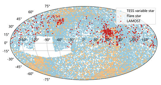
Figure 13.
Blue points represent the entire variable star sample, yellow points denote individual targets with flare events, and red points display the distribution of flare event targets observed by LAMOST.
4.2. Chromospheric Activity and Variation
Chromospheric activity refers to a series of phenomena occurring on the stellar surface, including changes in temperature and density and the formation of high-energy particles in the chromosphere. The H, H, H, H, and Ca II H&K spectral lines are usually used as indicators to measure the activity of stellar chromospheres. The DR9 dataset provides chromospheric activity indices, including the H equivalent width (EW), which is typically used to assess the activity level of a star. H is one of the most common lines in chromospheric activity, and its equivalent width reflects the degree of emission or absorption of hydrogen atoms on the stellar surface. As the activity on the star’s surface intensifies, the equivalent width of the H line rises, indicating the level of activity of the star. To determine the activity level of a star, the relationship between the H line equivalent width and the star’s surface temperature () is typically evaluated. In projects establishing activity criteria for stars, researchers have utilized multiple datasets to establish activity decision lines, including those by Fang et al. [74,75] based on LAMOST low-resolution spectra and Du et al. [76] based on the standard star catalog released by the LAMOST survey. We follow their criteria to assess the activity of our targets: the H equivalent width is greater than 0 and above our decision line. In Figure 14, we plot the distribution of H equivalent widths for variable stars in the 3000 K–4000 K temperature range, with the red line representing our activity decision line. Variable stars above the red line are considered active, while those below are inactive. Using this criterion, we identified 396 active stars among 398 low-resolution spectra containing H EW measurements. In Table 2, we denote the chromospheric activity of the stars, represented by “1” for active stars and “0” for inactive ones. We selected four samples with prominent H emissions from LAMOST low-resolution spectra, as shown in Figure 15. Figure 16 displays the relationship between the flare energy-to-luminosity ratio and the H equivalent width for 398 stars. Flares are closely related to H, as they enhance its features. The static radiation of H is produced by magnetic heating in the chromosphere. During flares, stressed magnetic field loops reconfigure to a lower-energy state, causing energy transfer and radiation, with some energy used to enhance H features [77,78]. We calculated the Pearson correlation coefficient between the flare-energy-to-luminosity ratio and equivalent width, with r = 0.275 and a p-value of . This means that as the H emission increases, so does the flare-energy-to-luminosity ratio to some extent, indicating the close relationship between flares and H. This result is consistent with previous studies [54].
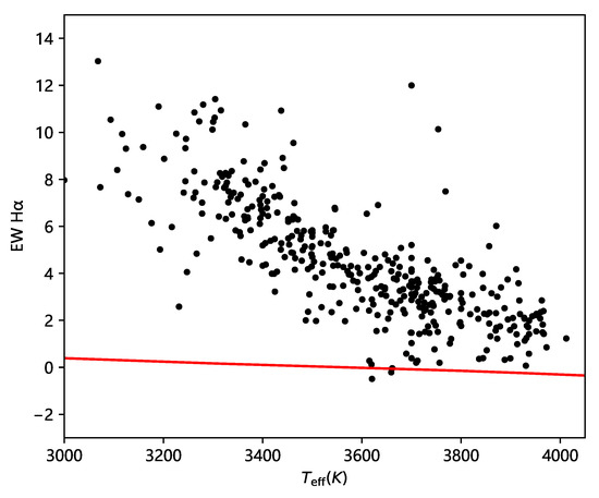
Figure 14.
Employing the activity diagnostic lines determined by standard stars (indicated by the red line), the sample is divided into active and inactive groups. Stars above the red line are considered active, while those below the line are deemed inactive.
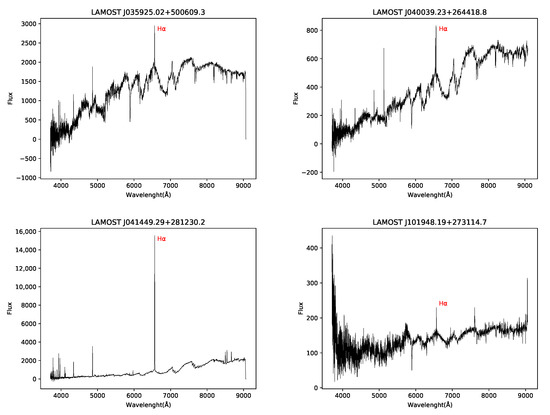
Figure 15.
The H emission line is displayed in the spectra of four stars observed at low resolution by LAMOST.
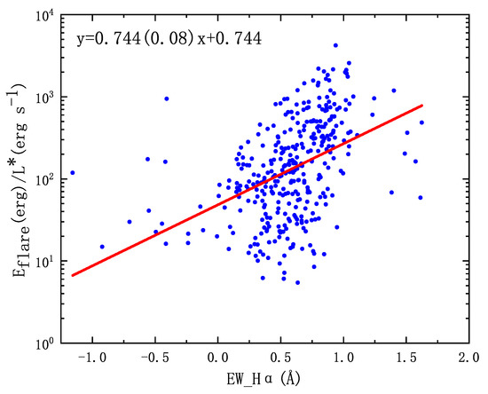
Figure 16.
The relationship between the ratio of flare energy to stellar luminosity and EWs of H.
5. Summary
We searched for flares in the light curves of stars by subtracting the background light curve obtained through polynomial fitting from the raw light curve. We discovered 25,327 flaring events in 3174 stars, including 245 eclipsing binaries, 2324 rotating stars, 111 pulsating stars, and 629 eruptive stars. It should be noted that the same star may have multiple type labels, so there may be some duplicated counts in these classifications. However, this has a limited impact on our overall conclusions. Using the TESS Input Catalog, we obtained the effective temperature and mass parameters for each target star and calculated the energy of each flare. For each event, we compiled a table of flare parameters, including the duration, amplitude, start and end time, and total energy. We performed statistical analysis on the flare parameters of the flaring events and found that 90% of the flares for all four types of variable stars had a duration of fewer than 2 h, and 91% had an amplitude of less than 0.3. The flare energy range ranged from erg to erg. Flare energy increased with increasing effective temperature and mass. There was a positive correlation between flare energy and duration and amplitude for different variable stars. The correlation between flare energy, duration, and amplitude was more pronounced for rotating and eruptive stars than for pulsating stars. The power-law index for the flare energy and duration of all the stars was 0.23. The power-law indices for rotating and eruptive stars were 0.27 and 0.26, respectively, which was similar to the value of around 1/3 for solar-like stars, indicating that the mechanisms behind most stellar flares are similar to those of solar flares. We conducted a statistical analysis of the number of flaring events for different types of variable stars. We found that the proportion of flaring stars is higher for rotating and eruptive stars than for eclipsing binaries and pulsating stars. The average number of flaring events for rotating and eruptive stars is also higher than for eclipsing binaries and pulsating stars. Regarding the temperature distribution of stars with flares, we observed that the proportion of stars exhibiting flares decreased with increasing temperature, with the majority of flares occurring in the temperature range of 2000–3000 K (accounting for 38.5% of all flares). For eclipsing binaries, the most common range for flares was 3000–4000 K, while for rotating, pulsating, and eruptive stars, they were more common in the range of 4000–5000 K.
We used maximum likelihood estimation to calculate the flare frequency distribution for different types of variable stars. The power-law index () was 1.72 ± 0.025, 1.82 ± 0.062, 1.80 ± 0.0116, and 1.73 ± 0.060 for eclipsing binaries, rotating stars, eruptive stars, and pulsating stars, respectively. The distribution range of these power-law indices was between 1.72 and 1.82, consistent with the results previously reported by other researchers [25,29,58]. We observed that the values were generally smaller for eclipsing binaries and pulsating stars and larger for rotating stars and eruptive stars. This indicates that, compared to rotating and eruptive stars or the entire sample, the flare energy of pulsating stars is more concentrated in the high-energy range. In terms of the flare occurrence rate, we found that 95% of variable stars had a flare occurrence rate of less than 5%, with the highest occurrence rate for eclipsing binaries and pulsating stars in the range of 0–1%, while for rotating and eruptive stars, it was in the range of 1–2%. We also identified 396 active stars using the H parameters provided by LAMOST DR9 and found a positive correlation between the H equivalent width and flare energy.
Author Contributions
Conceptualization, L.Z.; methodology, M.Z.; investigation, Z.Y. and T.S.; writing—review and editing, M.Z. All authors have read and agreed to the published version of the manuscript.
Funding
This research is funded by the Joint Fund of Astronomy of the NSFC and CAS Grant Nos. 11963002 and U1931132 and the China Manned Space Project Grant No. CMS-CSST-2021-B07. This research is also funded by the Cultivation Project for FAST Scientific Payoff Grant No. 2021.
Data Availability Statement
Not applicable.
Acknowledgments
Here, the first author would like to thank all the authors for their joint guidance, my teacher for his help and encouragement, and the reviewer for his valuable advice!
Conflicts of Interest
The authors declare no conflict of interest.
References
- Parker, E.N. The Solar-Flare Phenomenon and the Theory of Reconnection and Annihiliation of Magnetic Fields. Astrophys. J. Suppl. Ser. 1963, 8, 177. [Google Scholar] [CrossRef]
- Masuda, S.; Kosugi, T.; Hara, H.; Tsuneta, S.; Ogawara, Y. A loop-top hard X-ray source in a compact solar flare as evidence for magnetic reconnection. Nature 1994, 371, 495–497. [Google Scholar] [CrossRef]
- Su, Y.; Veronig, A.M.; Holman, G.D.; Dennis, B.R.; Wang, T.; Temmer, M.; Gan, W. Imaging coronal magnetic-field reconnection in a solar flare. Nat. Phys. 2013, 9, 489–493. [Google Scholar] [CrossRef]
- Maehara, H.; Shibayama, T.; Notsu, S.; Notsu, Y.; Nagao, T.; Kusaba, S.; Honda, S.; Nogami, D.; Shibata, K. Superflares on solar-type stars. Nature 2012, 485, 478–481. [Google Scholar] [CrossRef]
- Haisch, B.; Strong, K.T.; Rodono, M. Flares on the Sun and other stars. Annu. Rev. Astron. Astrophys. 1991, 29, 275–324. [Google Scholar] [CrossRef]
- Hawley, S.L.; Pettersen, B.R. The Great Flare of 1985 April 12 on AD Leonis. Astrophys. J. 1991, 378, 725. [Google Scholar] [CrossRef]
- Ambartsumian, V.A.; Mirzoian, L.V. Flare stars in star clusters and associations. In Symposium-International Astronomical Union, Volume 67: Variable Stars and Stellar Evolution; Sherwood, V.E., Plaut, L., Eds.; Reidel: Kufstein, Austria, 1975; pp. 3–14. [Google Scholar]
- Haro, G. The possible connexion between T Tauri stars and UV Ceti stars. In Symposium–International Astronomical Union, Volume 3: Non-Stable Stars; Herbig, G.H., Ed.; Cambridge University Press: Cambridge, UK, 1957; p. 26. [Google Scholar]
- Hilton, E.J. The Galactic M Dwarf Flare Rate. Ph.D. Thesis, University of Washington, Seattle, WA, USA, 2011. [Google Scholar]
- Rubenstein, E.P.; Schaefer, B.E. Are Superflares on Solar Analogues Caused by Extrasolar Planets? Astrophys. J. 2000, 529, 1031–1033. [Google Scholar] [CrossRef]
- Parsamyan, E.S. Dependence of the absolute magnitudes (energies) of flares on the age of the cluster in which the flare stars occur. Astrophysics 1976, 12, 145–151. [Google Scholar] [CrossRef]
- Parsamyan, E.S. Determination of the age of stellar aggregates and flare stars of the galactic field. Astrophysics 1995, 38, 206–212. [Google Scholar] [CrossRef]
- Borucki, W.J.; Koch, D.; Basri, G.; Batalha, N.; Brown, T.; Caldwell, D.; Caldwell, J.; Christensen-Dalsgaard, J.; Cochran, W.D.; DeVore, E.; et al. Kepler Planet-Detection Mission: Introduction and First Results. Science 2010, 327, 977. [Google Scholar] [CrossRef]
- Ricker, G.R.; Winn, J.N.; Vanderspek, R.; Latham, D.W.; Bakos, G.A.; Bean, J.L.; Berta-Thompson, Z.K.; Brown, T.M.; Buchhave, L.; Butler, N.R.; et al. Transiting Exoplanet Survey Satellite (TESS). In Proceedings of the Space Telescopes and Instrumentation 2014: Optical, Infrared, and Millimeter Wave, Montreal, QC, Canada, 22–27 June 2014; Oschmann Jacobus, M.J., Clampin, M., Fazio, G.G., MacEwen, H.A., Eds.; Volume 9143, p. 914320. [Google Scholar] [CrossRef]
- Wang, S.G.; Su, D.Q.; Chu, Y.Q.; Cui, X.; Wang, Y.N. Special configuration of a very large Schmidt telescope for extensive astronomical spectroscopic observation. Appl. Opt. 1996, 35, 5155–5161. [Google Scholar] [CrossRef] [PubMed]
- Su, D.Q.; Cui, X.Q. Active Optics in LAMOST. Chin. J. Astron. Astrophys. 2004, 4, 1–9. [Google Scholar] [CrossRef]
- Cui, X.Q.; Zhao, Y.H.; Chu, Y.Q.; Li, G.P.; Li, Q.; Zhang, L.P.; Su, H.J.; Yao, Z.Q.; Wang, Y.N.; Xing, X.Z.; et al. The Large Sky Area Multi-Object Fiber Spectroscopic Telescope (LAMOST). Res. Astron. Astrophys. 2012, 12, 1197–1242. [Google Scholar] [CrossRef]
- Koch, D.G.; Borucki, W.J.; Basri, G.; Batalha, N.M.; Brown, T.M.; Caldwell, D.; Christensen-Dalsgaard, J.; Cochran, W.D.; DeVore, E.; Dunham, E.W.; et al. Kepler Mission Design, Realized Photometric Performance, and Early Science. Astrophys. J. 2010, 713, L79–L86. [Google Scholar] [CrossRef]
- Jenkins, J.M. Initial Performance of the TESS Science Pipeline; American Astronomical Society: Washington, DC, USA, 2019. [Google Scholar]
- Walkowicz, L.M.; Basri, G.; Batalha, N.; Gilliland, R.L.; Jenkins, J.; Borucki, W.J.; Koch, D.; Caldwell, D.; Dupree, A.K.; Latham, D.W.; et al. White-light Flares on Cool Stars in the Kepler Quarter 1 Data. Astron. J. 2011, 141, 50. [Google Scholar] [CrossRef]
- Balona, L.A. Kepler observations of flaring in A–F type stars. Mon. Not. R. Astron. Soc. 2012, 423, 3420–3429. [Google Scholar] [CrossRef]
- Davenport, J.R.A.; Hawley, S.L.; Hebb, L.; Wisniewski, J.P.; Kowalski, A.F.; Johnson, E.C.; Malatesta, M.; Peraza, J.; Keil, M.; Silverberg, S.M.; et al. Kepler Flares. II. The Temporal Morphology of White-light Flares on GJ 1243. Astrophys. J. 2014, 797, 122. [Google Scholar] [CrossRef]
- Davenport, J.R.A. The Kepler Catalog of Stellar Flares. Astrophys. J. 2016, 829, 23. [Google Scholar] [CrossRef]
- Gao, Q.; Xin, Y.; Liu, J.F.; Zhang, X.B.; Gao, S. White-light Flares on Close Binaries Observed with Kepler. Astrophys. J. Suppl. Ser. 2016, 224, 37. [Google Scholar] [CrossRef]
- Lin, C.L.; Ip, W.H.; Hou, W.C.; Huang, L.C.; Chang, H.Y. A Comparative Study of the Magnetic Activities of Low-mass Stars from M-type to G-type. Astrophys. J. 2019, 873, 97. [Google Scholar] [CrossRef]
- Günther, M.N.; Zhan, Z.; Seager, S.; Rimmer, P.B.; Ranjan, S.; Stassun, K.G.; Oelkers, R.J.; Daylan, T.; Newton, E.; Kristiansen, M.H.; et al. Stellar Flares from the First TESS Data Release: Exploring a New Sample of M Dwarfs. Astron. J. 2020, 159, 60. [Google Scholar] [CrossRef]
- Ilin, E.; Schmidt, S.J.; Davenport, J.R.A.; Strassmeier, K.G. Flares in open clusters with K2. I. M 45 (Pleiades), M 44 (Praesepe), and M 67. Astron. Astrophys. 2019, 622, A133. [Google Scholar] [CrossRef]
- Feinstein, A.D.; Montet, B.T.; Ansdell, M.; Nord, B.; Bean, J.L.; Günther, M.N.; Gully-Santiago, M.A.; Schlieder, J.E. Flare Statistics for Young Stars from a Convolutional Neural Network Analysis of TESS Data. Astron. J. 2020, 160, 219. [Google Scholar] [CrossRef]
- Yang, Z.; Zhang, L.; Meng, G.; Han, X.L.; Misra, P.; Yang, J.; Pi, Q. Properties of flare events based on light curves from the TESS survey. Astron. Astrophys. 2023, 669, A15. [Google Scholar] [CrossRef]
- Parker, E.N. Cosmical Magnetic Fields. In Their Origin and Their Activity; Oxford University Press: Oxford, UK, 1979. [Google Scholar]
- Reiners, A.; Joshi, N.; Goldman, B. A Catalog of Rotation and Activity in Early-M Stars. Astron. J. 2012, 143, 93. [Google Scholar] [CrossRef]
- Douglas, S.T.; Agüeros, M.A.; Covey, K.R.; Bowsher, E.C.; Bochanski, J.J.; Cargile, P.A.; Kraus, A.; Law, N.M.; Lemonias, J.J.; Arce, H.G.; et al. The Factory and the Beehive. II. Activity and Rotation in Praesepe and the Hyades. Astrophys. J. 2014, 795, 161. [Google Scholar] [CrossRef]
- Fang, X.S.; Zhao, G.; Zhao, J.K.; Bharat Kumar, Y. Stellar activity with LAMOST—II. Chromospheric activity in open clusters. Mon. Not. R. Astron. Soc. 2018, 476, 908–926. [Google Scholar] [CrossRef]
- Yi, Z.; Luo, A.; Song, Y.; Zhao, J.; Shi, Z.; Wei, P.; Ren, J.; Wang, F.; Kong, X.; Li, Y.; et al. M Dwarf Catalog of the LAMOST Pilot Survey. Astron. J. 2014, 147, 33. [Google Scholar] [CrossRef]
- Chang, H.Y.; Song, Y.H.; Luo, A.L.; Huang, L.C.; Ip, W.H.; Fu, J.N.; Zhang, Y.; Hou, Y.H.; Cao, Z.H.; Wang, Y.F. LAMOST Observations of Flaring M Dwarfs in the Kepler Field. Astrophys. J. 2017, 834, 92. [Google Scholar] [CrossRef]
- Yang, H.; Liu, J.; Gao, Q.; Fang, X.; Guo, J.; Zhang, Y.; Hou, Y.; Wang, Y.; Cao, Z. The Flaring Activity of M Dwarfs in the Kepler Field. Astrophys. J. 2017, 849, 36. [Google Scholar] [CrossRef]
- Lu, H.p.; Zhang, L.y.; Shi, J.; Han, X.L.; Fan, D.; Long, L.; Pi, Q. Magnetic Activities of M-type Stars Based on LAMOST DR5 and Kepler and K2 Missions. Astrophys. J. Suppl. Ser. 2019, 243, 28. [Google Scholar] [CrossRef]
- Watson, C.L.; Henden, A.A.; Price, A. The International Variable Star Index (VSX). Soc. Astron. Sci. Annu. Symp. 2006, 25, 47. [Google Scholar]
- Ricker, G.R.; Winn, J.N.; Vanderspek, R.; Latham, D.W.; Bakos, G.A.; Bean, J.L.; Berta-Thompson, Z.K.; Brown, T.M.; Buchhave, L.; Butler, N.R.; et al. Transiting Exoplanet Survey Satellite (TESS). J. Astron. Telesc. Instrum. Syst. 2015, 1, 014003. [Google Scholar] [CrossRef]
- Jenkins, J.M. The Impact of Solar-like Variability on the Detectability of Transiting Terrestrial Planets. Astrophys. J. 2002, 575, 493–505. [Google Scholar] [CrossRef]
- Jenkins, J.M.; Chandrasekaran, H.; McCauliff, S.D.; Caldwell, D.A.; Tenenbaum, P.; Li, J.; Klaus, T.C.; Cote, M.T.; Middour, C. Transiting planet search in the Kepler pipeline. In Proceedings of the Software and Cyberinfrastructure for Astronomy, San Diego, CA, USA, 27–30 June 2010; Radziwill, N.M., Bridger, A., Eds.; Volume 7740, p. 77400D. [Google Scholar] [CrossRef]
- Jenkins, J.M.; Twicken, J.D.; McCauliff, S.; Campbell, J.; Sanderfer, D.; Lung, D.; Mansouri-Samani, M.; Girouard, F.; Tenenbaum, P.; Klaus, T.; et al. The TESS science processing operations center. In Proceedings of the Software and Cyberinfrastructure for Astronomy IV, Edinburgh, UK, 26–30 June 2016; Chiozzi, G., Guzman, J.C., Eds.; Volume 9913, p. 99133E. [Google Scholar] [CrossRef]
- Abdo, A.A.; Ackermann, M.; Agudo, I.; Ajello, M.; Allafort, A.; Aller, H.D.; Aller, M.F.; Antolini, E.; Arkharov, A.A.; Axelsson, M.; et al. Fermi Large Area Telescope and Multi-wavelength Observations of the Flaring Activity of PKS 1510-089 between 2008 September and 2009 June. Astrophys. J. 2010, 721, 1425–1447. [Google Scholar] [CrossRef]
- Abdo, A.A.; Ackermann, M.; Ajello, M.; Baldini, L.; Ballet, J.; Barbiellini, G.; Bastieri, D.; Bechtol, K.; Bellazzini, R.; Berenji, B.; et al. Multi-wavelength Observations of the Flaring Gamma-ray Blazar 3C 66A in 2008 October. Astrophys. J. 2011, 726, 43. [Google Scholar] [CrossRef]
- Davenport, J.R.A.; Covey, K.R.; Clarke, R.W.; Boeck, A.C.; Cornet, J.; Hawley, S.L. The Evolution of Flare Activity with Stellar Age. Astrophys. J. 2019, 871, 241. [Google Scholar] [CrossRef]
- Wu, C.J.; Ip, W.H.; Huang, L.C. A Study of Variability in the Frequency Distributions of the Superflares of G-type Stars Observed by the Kepler Mission. Astrophys. J. 2015, 798, 92. [Google Scholar] [CrossRef]
- Van Doorsselaere, T.; Shariati, H.; Debosscher, J. Stellar Flares Observed in Long-cadence Data from the Kepler Mission. Astrophys. J. Suppl. Ser. 2017, 232, 26. [Google Scholar] [CrossRef]
- Huang, L.C.; Ip, W.H.; Lin, C.L.; Zhang, X.L.; Song, Y.H.; Luo, A.L. M-dwarf Eclipsing Binaries with Flare Activity. Astrophys. J. 2020, 892, 58. [Google Scholar] [CrossRef]
- Günther, M.N.; Pozuelos, F.J.; Dittmann, J.A.; Dragomir, D.; Kane, S.R.; Daylan, T.; Feinstein, A.D.; Huang, C.X.; Morton, T.D.; Bonfanti, A.; et al. A super-Earth and two sub-Neptunes transiting the nearby and quiet M dwarf TOI-270. Nat. Astron. 2019, 3, 1099–1108. [Google Scholar] [CrossRef]
- Shporer, A.; Fuller, J.; Isaacson, H.; Hambleton, K.; Thompson, S.E.; Prša, A.; Kurtz, D.W.; Howard, A.W.; O’Leary, R.M. Radial Velocity Monitoring of Kepler Heartbeat Stars. Astrophys. J. 2016, 829, 34. [Google Scholar] [CrossRef]
- Webb, S.; Lochner, M.; Muthukrishna, D.; Cooke, J.; Flynn, C.; Mahabal, A.; Goode, S.; Andreoni, I.; Pritchard, T.; Abbott, T.M.C. Unsupervised machine learning for transient discovery in deeper, wider, faster light curves. Mon. Not. R. Astron. Soc. 2020, 498, 3077–3094. [Google Scholar] [CrossRef]
- Lochner, M.; Bassett, B.A. ASTRONOMALY: Personalised active anomaly detection in astronomical data. Astron. Comput. 2021, 36, 100481. [Google Scholar] [CrossRef]
- Vida, K.; Roettenbacher, R.M. Finding flares in Kepler data using machine-learning tools. Astron. Astrophys. 2018, 616, A163. [Google Scholar] [CrossRef]
- Su, T.; Zhang, L.y.; Long, L.; Han, X.L.; Misra, P.; Meng, G.; Pi, Q.; Yang, Z.; Yang, J. Magnetic Activity and Physical Parameters of Exoplanet Host Stars Based on LAMOST DR7, TESS, Kepler, and K2 Surveys. Astrophys. J. Suppl. Ser. 2022, 261, 26. [Google Scholar] [CrossRef]
- Tu, Z.L.; Yang, M.; Wang, H.F.; Wang, F.Y. Superflares, Chromospheric Activities, and Photometric Variabilities of Solar-type Stars from the Second-year Observation of TESS and Spectra of LAMOST. Astrophys. J. Suppl. Ser. 2021, 253, 35. [Google Scholar] [CrossRef]
- Notsu, Y.; Maehara, H.; Honda, S.; Hawley, S.L.; Davenport, J.R.A.; Namekata, K.; Notsu, S.; Ikuta, K.; Nogami, D.; Shibata, K. Do Kepler Superflare Stars Really Include Slowly Rotating Sun-like Stars?—Results Using APO 3.5 m Telescope Spectroscopic Observations and Gaia-DR2 Data. Astrophys. J. 2019, 876, 58. [Google Scholar] [CrossRef]
- Berger, T.A.; Huber, D.; Gaidos, E.; van Saders, J.L. Revised Radii of Kepler Stars and Planets Using Gaia Data Release 2. Astrophys. J. 2018, 866, 99. [Google Scholar] [CrossRef]
- Yang, H.; Liu, J. The Flare Catalog and the Flare Activity in the Kepler Mission. Astrophys. J. Suppl. Ser. 2019, 241, 29. [Google Scholar] [CrossRef]
- Stassun, K.G.; Oelkers, R.J.; Pepper, J.; Paegert, M.; De Lee, N.; Torres, G.; Latham, D.W.; Charpinet, S.; Dressing, C.D.; Huber, D.; et al. The TESS Input Catalog and Candidate Target List. Astron. J. 2018, 156, 102. [Google Scholar] [CrossRef]
- Huber, D.; Silva Aguirre, V.; Matthews, J.M.; Pinsonneault, M.H.; Gaidos, E.; García, R.A.; Hekker, S.; Mathur, S.; Mosser, B.; Torres, G.; et al. Revised Stellar Properties of Kepler Targets for the Quarter 1–16 Transit Detection Run. Astrophys. J. Suppl. Ser. 2014, 211, 2. [Google Scholar] [CrossRef]
- Skrutskie, M.F.; Cutri, R.M.; Stiening, R.; Weinberg, M.D.; Schneider, S.; Carpenter, J.M.; Beichman, C.; Capps, R.; Chester, T.; Elias, J.; et al. The Two Micron All Sky Survey (2MASS). Astron. J. 2006, 131, 1163–1183. [Google Scholar] [CrossRef]
- Zacharias, N.; Finch, C.T.; Girard, T.M.; Henden, A.; Bartlett, J.L.; Monet, D.G.; Zacharias, M.I. The Fourth US Naval Observatory CCD Astrograph Catalog (UCAC4). Astron. J. 2013, 145, 44. [Google Scholar] [CrossRef]
- Paegert, M.; Stassun, K.G.; De Lee, N.; Pepper, J.; Fleming, S.W.; Sivarani, T.; Mahadevan, S.; Mack Claude, E.I.; Dhital, S.; Hebb, L.; et al. Target Selection for the SDSS-III MARVELS Survey. Astron. J. 2015, 149, 186. [Google Scholar] [CrossRef]
- Wright, E.L.; Eisenhardt, P.R.M.; Mainzer, A.K.; Ressler, M.E.; Cutri, R.M.; Jarrett, T.; Kirkpatrick, J.D.; Padgett, D.; McMillan, R.S.; Skrutskie, M.; et al. The Wide-field Infrared Survey Explorer (WISE): Mission Description and Initial On-orbit Performance. Astron. J. 2010, 140, 1868–1881. [Google Scholar] [CrossRef]
- Samus’, N.N.; Kazarovets, E.V.; Durlevich, O.V.; Kireeva, N.N.; Pastukhova, E.N. General catalogue of variable stars: Version GCVS 5.1. Astron. Rep. 2017, 61, 80–88. [Google Scholar] [CrossRef]
- Tu, Z.L.; Yang, M.; Zhang, Z.J.; Wang, F.Y. Superflares on Solar-type Stars from the First Year Observation of TESS. Astrophys. J. 2020, 890, 46. [Google Scholar] [CrossRef]
- Jackman, J.A.G.; Wheatley, P.J.; Acton, J.S.; Anderson, D.R.; Bayliss, D.; Briegal, J.T.; Burleigh, M.R.; Casewell, S.L.; Gänsicke, B.T.; Gill, S.; et al. Stellar flares detected with the Next Generation Transit Survey. Mon. Not. R. Astron. Soc. 2021, 504, 3246–3264. [Google Scholar] [CrossRef]
- Goldstein, M.L.; Morris, S.A.; Yen, G.G. Problems with fitting to the power-law distribution. Eur. Phys. J. B 2004, 41, 255–258. [Google Scholar] [CrossRef]
- Newman, M.E.J. Power laws, Pareto distributions and Zipf’s law. Contemp. Phys. 2005, 46, 323–351. [Google Scholar] [CrossRef]
- Bauke, H. Parameter estimation for power-law distributions by maximum likelihood methods. Eur. Phys. J. B 2007, 58, 167–173. [Google Scholar] [CrossRef]
- Li, Y.P. Fitting Power-law Frequency Distribution with a Modified Maximum Likelihood Estimator. Acta Astron. Sin. 2014, 55, 437–443. [Google Scholar]
- Shibata, K.; Takasao, S. Fractal Reconnection in Solar and Stellar Environments. In Magnetic Reconnection: Concepts and Applications; Gonzalez, W., Parker, E., Eds.; Springer: Cham, Switzerland, 2016; Volume 427, p. 373. [Google Scholar] [CrossRef]
- Shibayama, T.; Maehara, H.; Notsu, S.; Notsu, Y.; Nagao, T.; Honda, S.; Ishii, T.T.; Nogami, D.; Shibata, K. Superflares on Solar-type Stars Observed with Kepler. I. Statistical Properties of Superflares. Astrophys. J. Suppl. Ser. 2013, 209, 5. [Google Scholar] [CrossRef]
- Fang, X.S.; Zhao, G.; Zhao, J.K.; Chen, Y.Q.; Bharat Kumar, Y. Stellar activity with LAMOST—I. Spot configuration in Pleiades. Mon. Not. R. Astron. Soc. 2016, 463, 2494–2512. [Google Scholar] [CrossRef]
- Fang, X.S.; Bidin, C.M.; Zhao, G.; Zhang, L.Y.; Bharat Kumar, Y. Stellar activity with LAMOST. III. Temporal variability pattern in Pleiades, Praesepe, and Hyades. Mon. Not. R. Astron. Soc. 2020, 495, 2949–2965. [Google Scholar] [CrossRef]
- Du, B.; Luo, A.L.; Zuo, F.; Bai, Z.R.; Wang, R.; Song, Y.H.; Hou, W.; Li, Y.B.; Zhang, J.N.; Guo, Y.X.; et al. An Empirical Template Library for FGK and Late-type A Stars Using LAMOST Observed Spectra. Astrophys. J. Suppl. Ser. 2019, 240, 10. [Google Scholar] [CrossRef]
- Kruse, E.A.; Berger, E.; Knapp, G.R.; Laskar, T.; Gunn, J.E.; Loomis, C.P.; Lupton, R.H.; Schlegel, D.J. Chromospheric Variability in Sloan Digital Sky Survey M Dwarfs. II. Short-timescale Hα Variability. Astrophys. J. 2010, 722, 1352–1359. [Google Scholar] [CrossRef]
- Bell, K.J.; Hilton, E.J.; Davenport, J.R.A.; Hawley, S.L.; West, A.A.; Rogel, A.B. Hα Emission Variability in Active M Dwarfs. Publ. Astron. Soc. Pac. 2012, 124, 14. [Google Scholar] [CrossRef]


Disclaimer/Publisher’s Note: The statements, opinions and data contained in all publications are solely those of the individual author(s) and contributor(s) and not of MDPI and/or the editor(s). MDPI and/or the editor(s) disclaim responsibility for any injury to people or property resulting from any ideas, methods, instructions or products referred to in the content. |
© 2023 by the authors. Licensee MDPI, Basel, Switzerland. This article is an open access article distributed under the terms and conditions of the Creative Commons Attribution (CC BY) license (https://creativecommons.org/licenses/by/4.0/).