Anisotropy of Self-Correlation Level Contours in Three-Dimensional Magnetohydrodynamic Turbulence

Abstract

MHD turbulence is considered to be anisotropic owing to the presence of a magnetic field, and its self-correlation anisotropy has been unveiled by solar wind observations. Here, based on numerical results of compressible MHD turbulence with a global mean magnetic field, we explore variations of the normalized self-correlation function’s (NCF) level contours with the scale as well as their evolution. The analyses reveal that the NCF’s level contours tend to elongate in the direction parallel to the mean magnetic field, and the elongation becomes weak with decreasing intervals. These results are consistent with slow solar wind observations. The less anisotropy of the NCF’s level contours with the shorter intervals can be produced by the fact that coherent structures stretch more along the parallel direction at the long intervals than at the short intervals. The analyses also disclose that as the simulation time builds up, the NCF’s level contours change thinner and thinner, and the anisotropy of the NCF’s level contours grows, which can be caused by the break of large coherent structures into small ones. The increased self-correlation anisotropy with time foretells that the self-correlation anisotropy of solar wind turbulence enlarges with the radial distance, which needs to be tested against observations by using Parker Solar Probe (PSP) measurements.

1. Introduction

Unlike homogeneous hydrodynamic (HD) turbulence, magnetohydrodynamic (MHD) turbulence is threaded by a background magnetic field. The magnetic field determines a peculiar direction and tends to make MHD turbulence different in the directions parallel and perpendicular to the magnetic field [1,2,3,4]. The anisotropy of MHD turbulence has impacts on the cascading of turbulent energy, the heating of interplanetary plasma, the propagation and scattering of cosmic rays, and other astrophysical phenomena. Solar wind fluctuations have a magnetic field frozen in it, and are a natural laboratory to study anisotropy owing to the presence of a magnetic field [5,6,7].

To measure the anisotropy of solar wind turbulence with respect to the global mean field, ${\mathbf{B}}_{\mathbf{0}}$, or to the local mean field, ${\mathbf{B}}_{\mathbf{l}}$, in the inertia range, researchers employ various tools, such as correlation functions [8,9,10,11,12,13,14,15,16,17,18], structure functions [19,20,21,22,23,24,25], wavelet [26,27,28,29,30,31], and so on. Ref. [9] constructed a two-dimensional (2D) correlation function for a magnetic field, and gave the first results that show that level contours of magnetic self-correlation have a cross-like shape, called the Maltese cross. This pattern was interpreted as a superposition of slab and 2D fluctuations. After that, the self-correlation anisotropy of solar wind turbulence was testified by both single- and multi-satellite observations [10,11,12,13,15], and it was a broad agreement that the level contours of magnetic and velocity self-correlation elongate along the mean field direction at long durations. Aiming to check how self-correlation anisotropy changes with scale, ref. [16] showed that level contours of the normalized self-correlation function (NCF) become close to isotropic for shorter intervals from about 10 h to 1 h.

Using moments of increments, the structure function can probe power levels and is often used to quantify the scaling law in turbulence [32]. To understand the variation in solar wind turbulence anisotropy with scale, the local mean field ${\mathbf{B}}_{\mathbf{l}}$ is introduced and calculated as the average of magnetic fields at two points. With this method, solar wind fluctuations are revealed to be anisotropic in spectral index and power level, which are functions of the angle ${\theta }_{VB}$ between the flow direction and the direction of ${\mathbf{B}}_{\mathbf{l}}$. The related results are what are expected from a critical balance cascade [2,33]. Furthermore, people extend 2D anisotropic studies to a three-dimensional (3D) scenario, which includes the local mean magnetic field direction, the perpendicular magnetic field fluctuation direction, and the direction perpendicular to both, and a power-law index of about $1/2$ was found in the perpendicular direction [20,24].

Meanwhile, numerical works have been conducted to study the anisotropy of MHD turbulence [1,34,35,36,37,38,39,40,41,42,43,44,45,46,47,48,49,50,51,52]. Shebalin angle, ${\theta }_Q$, is employed to quantify anisotropy of the MHD turbulence, and is defined as ${tan}^2{\theta }_Q=\left(\sum k_{\perp }^2{\left|\mathit{Q}\left(\mathit{k}\right)\right|}^2\right)/\left(\sum k_{\parallel }^2{\left|\mathit{Q}\left(\mathit{k}\right)\right|}^2\right)$, where $\mathit{Q}\left(\mathit{k}\right)$ is a vector field, $\mathit{k}$ is the wave vector, and $k_{\perp }$ and $k_{\parallel }$ are wavenumbers in the perpendicular and parallel directions, respectively. Ref. [35] found that the anisotropy, revealed by ${\theta }_Q$, is more pronounced at small scales. However, ref. [38] presented the scale independence of the anisotropy from the contours of energy spectra $E\left(k_{\perp },k_{\parallel }\right)/E\left(k_{\perp },0\right)$ in the $\left(k_{\perp },k_{\parallel }\right)-$plane.

Different from the above techniques that measure anisotropy relative to the global mean magnetic field, ${\mathbf{B}}_{\mathbf{0}}$, [38,39] suggested that anisotropy should be measured relative to the local mean field, ${\mathbf{B}}_{\mathbf{l}}$. By calculating the second-order structure function tied to ${\mathbf{B}}_{\mathbf{l}}$, they found that the anisotropy of the MHD turbulence conforms to the scaling laws predicted by the critical balance scenario. Ref. [48] pointed out that solar wind expansion should be taken into account to match the modeled 3D anisotropy of the structure function in MHD turbulence to that observed in the solar wind. Ref. [51] employed the wavelet tool to investigate the spectral anisotropy of the MHD turbulence, and they obtained power-law spectra with an index of about $-5/3$ in the perpendicular direction and about $-2$ in the parallel direction, similar to solar wind observations. Ref. [52] showed that for the large-amplitude MHD turbulence, the scaling of multi-order structure functions displays a multifractal scaling at all angles to ${\mathbf{B}}_{\mathbf{l}}$, with probability distribution functions (PDFs) deviating significantly from Gaussian distribution and flatness larger than 3.

Until now, the self-correlation anisotropy has not been systematically investigated in numerical simulations of MHD turbulence. In this work, we investigate the anisotropy of the NCF’s level contours for magnetic field and velocity to understand their variations with the scale as well as their evolution. The paper is organized as follows: In Section 2, we describe the setting of our numerical simulation parameters as well as the sampling methods. In Section 3, we present our numerical results, and in Section 4, we give a brief concluding remarks and discuss their implications.

2. Numerical Mhd Model

The 3D compressible MHD model used in this paper was detailed in [53,54], and the governing equations read as follows:

$$\frac{\partial \rho }{\partial t}+\nabla ·\left(\rho \mathbf{u}\right)=0,$$

(1)

$$\frac{\partial \rho \mathbf{u}}{\partial t}+\nabla ·\left[\rho \mathbf{u}\mathbf{u}+(p+\frac{1}{2}{\mathbf{B}}^2)\mathbf{I}-\mathbf{B}\mathbf{B}\right]=\nu {\nabla }^2\mathbf{u}+\rho ·({\mathbf{f}}_1-{\mathbf{f}}_2),$$

(2)

$$\frac{\partial e}{\partial t}+\nabla ·\left[(e+p+\frac{1}{2}{\mathbf{B}}^2)\mathbf{u}-(\mathbf{u}·\mathbf{B})\mathbf{B}\right]=\nabla ·(\mathbf{u}·\nu \nabla \mathbf{u})+\nabla ·(\mathbf{B}\times \eta \mathbf{j})+\rho \mathbf{u}·({\mathbf{f}}_1-{\mathbf{f}}_2)+\mathbf{B}·({\mathbf{f}}_1+{\mathbf{f}}_2),$$

(3)

$$\frac{\partial \mathbf{B}}{\partial t}+\nabla ·(\mathbf{u}\mathbf{B}-\mathbf{B}\mathbf{u})=\eta {\nabla }^2\mathbf{B}+{\mathbf{f}}_1+{\mathbf{f}}_2,$$

(4)

with $e=(1/2)\rho {\mathbf{u}}^2+p/(\gamma -1)+(1/2){\mathbf{B}}^2,\mathbf{j}=\nabla \times \mathbf{B}$ corresponding to the total energy density and current density, respectively. Here, $\rho$ is the mass density; p is the thermal pressure; $\mathbf{u}$ is the the velocity field; $\mathbf{B}={\mathbf{B}}_{\mathbf{0}}+\mathbf{b}$ denotes the total magnetic field; t is time; $\gamma =5/3$ is the adiabatic index; $\nu =0.0001$ is the viscosity; $\eta =0.0001$ is the magnetic resistivity. The uniform global field ${\mathbf{B}}_0(=1.00)$ is imposed in the z-direction.

To normalize the MHD Equations (1)–(4), we choose three independent parameters, for example, a characteristic density ${\rho }_0$, a characteristic length $L_0$, and a characteristic Alfvén speed $v_{A0}$. Other variables are normalized by their combinations. The simulation data are thus dimensionless and in arbitrary units. In the following, the variables are plotted to be unitless. Certainly, we can use ${\rho }_0$, $L_0$, and $v_{A0}$ at 1 au to have the variables be dimensional, as carried out by [55].

Turbulence is driven at large scales by the forcers ${\mathbf{f}}_1$ and ${\mathbf{f}}_2$, which produce Alfvénic perturbations propagating anti-parallel and parallel to magnetic field, respectively. Both are isotropic and consist of 21 Fourier components with wavenumber $k⩽3.5$ and random phase angles [53,54]. After turbulent quantities reach a statistically quasi-stationary state, the root-mean-square (RMS) values for velocity and magnetic field in dimensionless form are approximately 0.62 and 0.54, respectively; cross-helicity ${\sigma }_c=0.42$, plasma beta $\beta =0.38$, and averaged Alfvén speed in dimensionless form $\langle V_A\rangle =1.00$. The state of turbulent quantities in [56] is utilized here, and the below analyses are conducted when the simulated turbulence is in the statistically quasi-stationary state.

Only the prior magnetic field ${\mathbf{B}}_0$ is used to initialize Equations (1)–(4), and the simulation starts from an initial state free of fluctuations. We consider periodic boundary conditions in a cube with a side length of $2\pi$ and a resolution defined by the number of grid points, which is ${1024}^3$. We apply a third-order piecewise parabolic method to the reconstruction and a approximate Riemann solver of Harten–Lax–van Leer discontinuities (HLLD) to the calculation of numerical fluxes. The constrained transport algorithm is employed to ensure the divergence-free state of the magnetic field.

3. Numerical Results

Figure 1 presents trace power spectra of the magnetic field $\mathbf{B}$ (blue) and the velocity $\mathbf{u}$ (red). From the figure, we can see that the trace power spectra of $\mathbf{B}$ and $\mathbf{u}$ show power laws with an index of about $-5/3$ in the range $4⩽k⩽40$, with k being the wavenumber. As there are no fluctuations at the initial time, energy injected at large scales by the forces is cascaded down into small scales. The range $4⩽k⩽40$ is considered as the inertial range of the driven turbulence. When $k<4$, it is the energy injection region, with energy peaked at about $k=3$.

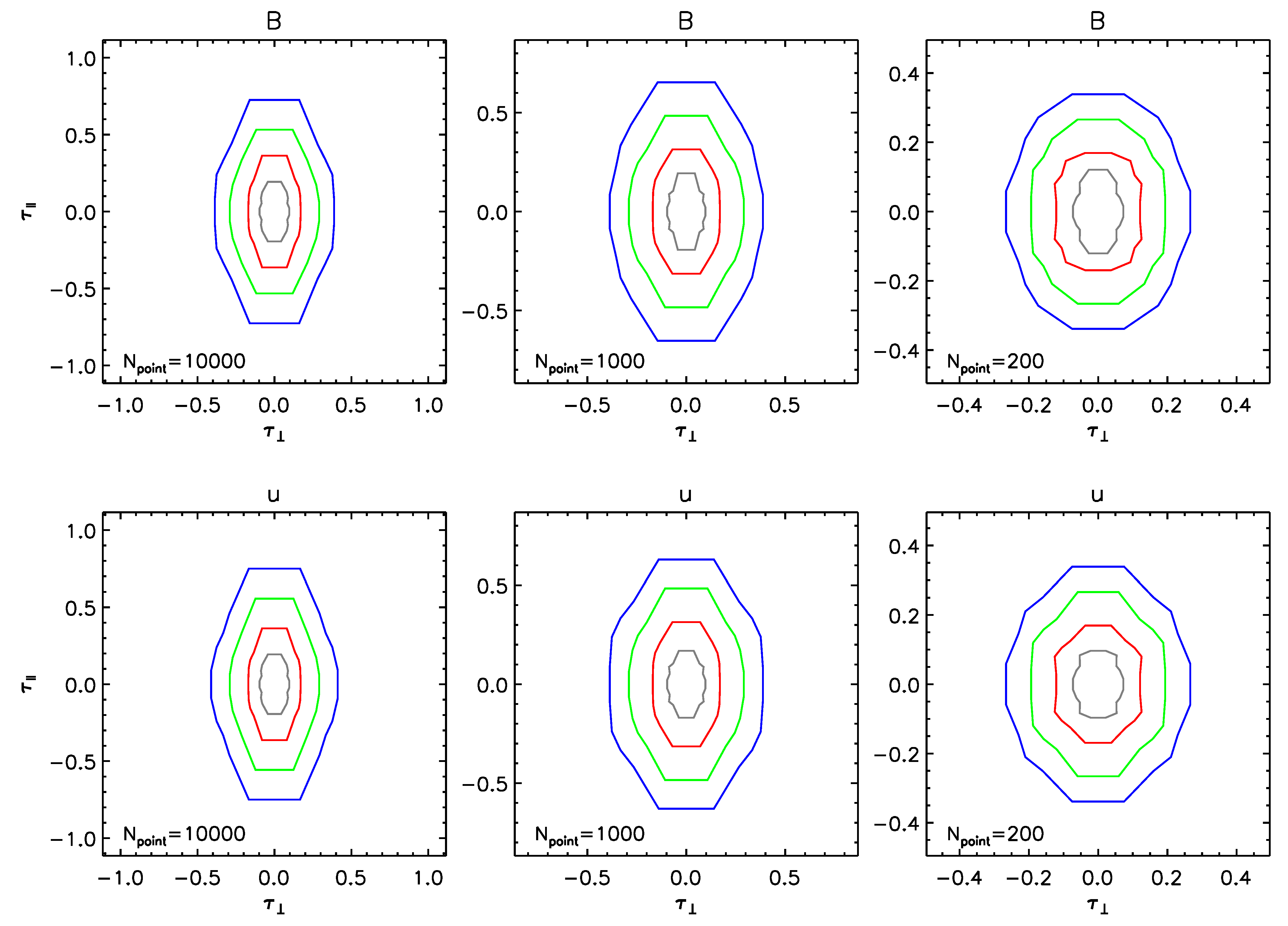
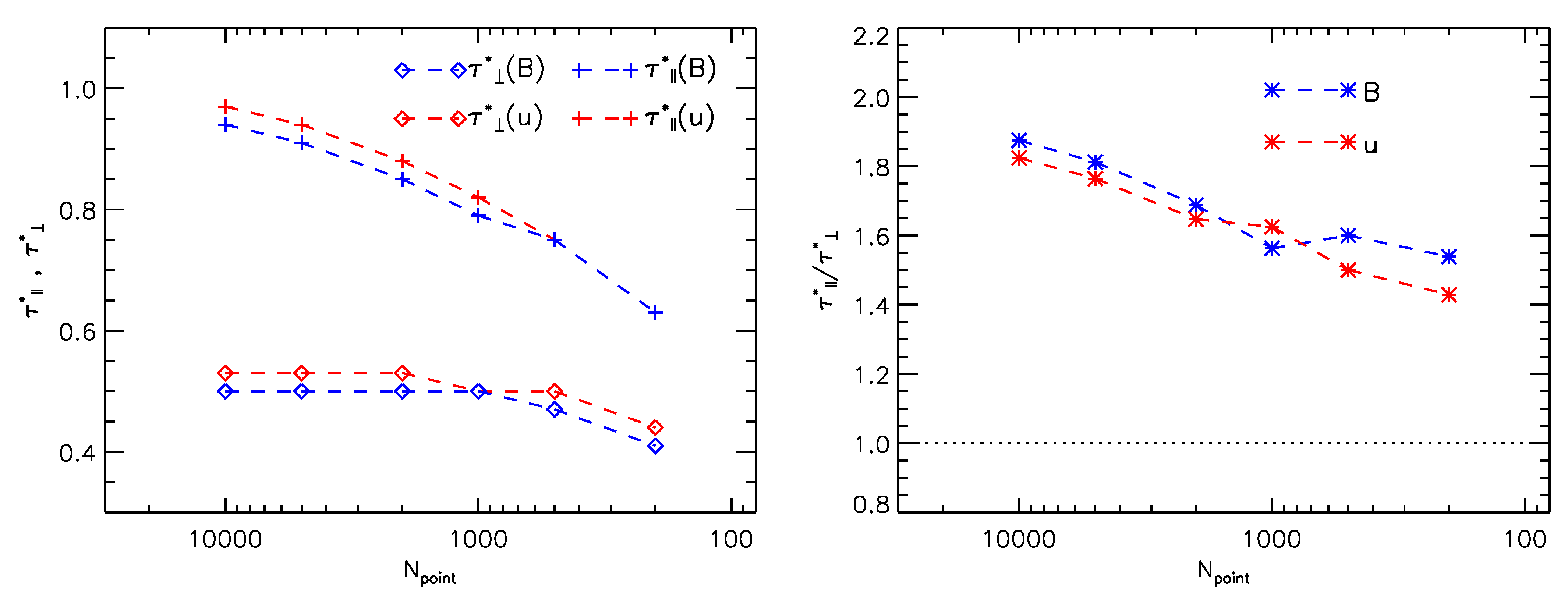
3.1. Anisotropy of the NCF’s Level Contours

To investigate the anisotropy of the NCF’s level contours, we first sample the numerical data with a virtual satellite, whose path is shown as white dashed lines in Figure 2. As periodic boundary conditions are used, the virtual satellite crosses the boundaries and reenters the computation domain many times. In total, about 2,000,000 points are sampled. With Taylor’s hypothesis [57], in situ spacecraft measurements in the solar wind can be converted from temporal to spatial scales. In view of the fact that both the virtual satellite and actual satellites in the solar wind obtain a sequence of the turbulent quantities, which can be thought to change in the spatial scales, our way to “probe“ the simulation data is similar to in situ measurements in the solar wind.

The sampled data are then cut into intervals with a duration of 500 points $(N_{\mathrm{point}}=500)$. As carried out in [16], the adjacent intervals are shifted by $N_{\mathrm{point}}/2$ to make as many points as possible be used to calculate self-correlation function. For each interval i, we compute a two-point self-correlation function of the vector $\mathit{U}$ with:

$$\mathrm{CF}(i,\tau )={\left.\langle \delta \mathit{U}(i,r)·\delta \mathit{U}(i,r+\tau )\rangle \right|}_r$$

(5)

where $\mathit{U}$ can be velocity and magnetic field; $\delta \mathit{U}$ is defined as $\delta \mathit{U}=\mathit{U}-\overline{\mathit{U}}$, with $\overline{\mathit{U}}$ denoting the vector whose components are linear fits to the corresponding components of $\mathit{U}$; $\tau =0,\Delta ,2\Delta ,\dots ,R/2$ is spatial lag, with $\Delta$ being the distance between two adjacent sampled points and R being the length of the intervals; and ${\langle \dots \rangle |}_r$ means an average over the points of the interval i. We also use a variance-based normalization factor $\lambda \left(i\right)$ to compute the normalized self-correlation function by $\mathrm{NCF}(i,\tau )=\lambda \left(i\right)\mathrm{CF}(i,\tau )$ with $\lambda \left(i\right)=\mathrm{CF}\left(0\right)/\mathrm{CF}(i,0)$. Here, $\mathrm{CF}\left(0\right)$ denotes the average of $\mathrm{CF}(i,0)$ for all of the intervals.

Finally, we compute a mean magnetic field for each interval, and define an angle between the sampling direction and the mean field direction, ${\theta }_{RB}$, in order to study the anisotropy of the NCF. Considering that the sampling direction remains unchanged, each interval has only one ${\theta }_{RB}$. According to the values of ${\theta }_{RB}$, all of the intervals are classified into five groups, i.e., $0^{\circ }⩽{\theta }_{RB}<{25}^{\circ }$, ${25}^{\circ }⩽\theta <{40}^{\circ },{40}^{\circ }⩽\theta <{50}^{\circ },{50}^{\circ }⩽\theta <{65}^{\circ },$ and ${65}^{\circ }⩽{\theta }_{RB}⩽{90}^{\circ }$. In each group, we average the NCFs, and mark the average value with the middle value of the angle ranges ${\theta }_{RBj}=\left({\theta }_{RBj,min}+{\theta }_{RBj,max}\right)/2(j=1,2,\dots ,5)$:

$$NCF\left({\theta }_{RBj},\tau \right)=\frac{1}{n\left({\theta }_{RBj}\right)}\sum _{{\theta }_{RBj,min}⩽{\theta }_{RB}\left(i\right)<{\theta }_{RBj,max}}NCF(i,\tau )$$

where $n\left({\theta }_{RBj}\right)$ is the number of the intervals, where the condition of ${\theta }_{RBj,min}⩽{\theta }_{RB}\left(i\right)<{\theta }_{RBj,max}$ holds.

In Figure 3, we present the variation in the $\mathrm{NCF}$s with the spatial lag $\tau$ for the angle ranges ${65}^{\circ }⩽{\theta }_{RB}⩽{90}^{\circ }$ and $0^{\circ }⩽{\theta }_{RB}<{25}^{\circ }$ for the intervals with a duration of $N_{\mathrm{point}}=500$. At the same value of the $\mathrm{NCF}$, the difference of $\tau$ on two curves indicates the anisotropy of the self-correlation function. In the parallel direction ($0^{\circ }⩽{\theta }_{RB}<{25}^{\circ }$), the value of $\tau$ is always larger than that in the perpendicular direction (${65}^{\circ }⩽{\theta }_{RB}⩽{90}^{\circ }$), which means that the NCF’s level contours are elongated in the parallel direction for the intervals with the 500-point length.

In the lower panels of Figure 3, we give count distributions of the magnetic $\mathrm{NCF}$ at the mean value of $e^{-1}$ for the angle ranges ${65}^{\circ }⩽{\theta }_{RB}⩽{90}^{\circ }$ and $0^{\circ }⩽{\theta }_{RB}<{25}^{\circ }$, with the averages and standard deviations marked in the expression. They conform to Gaussian distribution, with small standard deviation, which suggests that the average values of the magnetic $\mathrm{NCF}$ shown in the upper panel can be used as the representation of the NCFs in each group of ${\theta }_{RBj}$.

To understand the variation in the NCF’s level contours with the interval length, we redo the above analysis but using different lengths of intervals with $N_{\mathrm{point}}=$10,000, 5000, 2000, 1000, and 200. Figure 4 presents the NCF’s level contours of the magnetic field and the velocity on the 2D (${\tau }_{\parallel },{\tau }_{\perp }$) plane for $N_{\mathrm{point}}$ = 10,000, 1000, and 200, where ${\tau }_{\parallel }$ and ${\tau }_{\perp }$ are the spatial lags in the direction parallel and perpendicular to the mean field, respectively.

Figure 4 exhibits that as the lengths of the intervals drop, the elongation of the NCF’s level contours along the parallel direction becomes weak, and the NCF’s level contours are closer to a circle. This indicates that the anisotropy of the NCF’s level contours decreases when the intervals become short. As expected, the level contours of the magnetic NCF have a similar shape to those of the velocity NCF at a given scale.

The left panel of Figure 5 presents the spatial lags ${\tau }_{\parallel }^{\ast }$ and ${\tau }_{\perp }^{\ast }$ at the different lengths of the intervals for the magnetic field and the velocity. Here, ${\tau }_{\parallel }^{\ast }$ and ${\tau }_{\perp }^{\ast }$ are the values corresponding to NCF$(0,{\tau }_{\parallel }^{\ast })=e^{-1}$ and NCF$({\tau }_{\perp }^{\ast },0)=e^{-1}$, respectively. We can find that as the lengths of the intervals decrease, ${\tau }_{\parallel }^{\ast }$ drops quickly, while ${\tau }_{\perp }^{\ast }$ changes gently. This results in the anisotropy ratio, ${\tau }_{\parallel }^{\ast }/{\tau }_{\perp }^{\ast }$, to increase with the length of the intervals, as shown in the right panel of Figure 5.

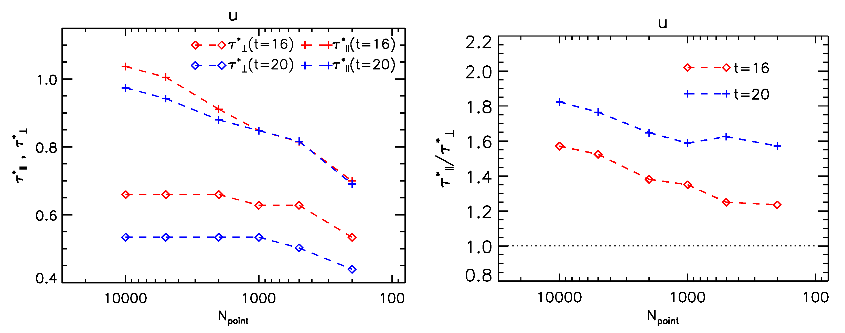
3.2. Evolution of the NCF’s Level Contours

In this subsection, we examine the time evolution of the NCF’s level contours in order to foretell the radial evolution of the self-correlation anisotropy of solar wind turbulence, which could be tested against observations by using Parker Solar Probe (PSP) measurements.

Figure 6 displays the time evolution of the kinetic and magnetic energies, which are computed according to fluctuations of the velocity and magnetic field. After the simulation begins, the kinetic and magnetic energies rise quickly. At $t\sim 5$, the kinetic and magnetic energies of the $z-$component, $E_{\mathrm{dvz}}$ and $E_{\mathrm{dbz}}$, begin to settle down, while the kinetic and magnetic energies of the $y-$component, $E_{\mathrm{dvy}}$ and $E_{\mathrm{dby}}$ steadily creep up until $t\sim 15$. Afterwards, the energies appear to reach a steady value, and the driven turbulence is in the statistically quasi-stationary state. As the uniform global field ${\mathbf{B}}_0$ is imposed in the z-direction, $E_{\mathrm{dvy}}$ and $E_{\mathrm{dby}}$ can be regarded as the noncompressible energies, and $E_{\mathrm{dvz}}$ and $E_{\mathrm{dbz}}$ are compressible energies. At the statistically quasi-stationary state, it can be seen that the noncompressible energies are greater than the compressible energies.

After the simulated turbulence gets into the statistically quasi-stationary state, we use the same procedures as described in Section 3.1 to compute $\mathrm{NCF}(i,\tau )$ as well as its variation with the angle ${\theta }_{RB}$, i.e., $NCF\left({\theta }_{RB},\tau \right)$. Figure 7 presents the NCF’s level contours of the velocity at 10,000-, 1000-, and 200-point lengths of intervals on the 2D (${\tau }_{\parallel },{\tau }_{\perp }$) plane for $t=16$ and 20, when the NCF’s level contours are also elongated along the parallel direction, and the elongation becomes weak with the decreased intervals. Compared to those at $t=16$, the NCF’s level contours tend to be thinner at $t=20$, meaning the increased anisotropy of the NCF’s level contours with the time.

To measure the anisotropy of the NCF’s level contours as well as its evolution, Figure 8 presents variations of the spatial lags ${\tau }_{\parallel }^{\ast }$ and ${\tau }_{\perp }^{\ast }$ and the anisotropy ratio ${\tau }_{\parallel }^{\ast }/{\tau }_{\perp }^{\ast }$ with the length of the intervals for the velocity. It can be learnt that from the long to the short intervals, ${\tau }_{\perp }^{\ast }$ at $t=16$ keeps larger than ${\tau }_{\perp }^{\ast }$ at $t=20$, while only at the long intervals, ${\tau }_{\parallel }^{\ast }$ at $t=16$ is larger than ${\tau }_{\parallel }^{\ast }$ at $t=20$. The anisotropy ratio ${\tau }_{\parallel }^{\ast }/{\tau }_{\perp }^{\ast }$, shown at the right panel of Figure 8, thus grows with the time. It is remarked that the anisotropy of the magnetic NCFs has a similar evolution to that of the velocity NCFs at a given scale.

Figure 9 displays the distributions of the fluctuations of the velocity component $v_y$ on the $x-y$ and $x-z$ planes for $t=16$. From this figure, we can detect some clues to the decreased self-correlation anisotropy with the scale. It is noted that coherent structures, which are rendered in red or dark purple, stretch not only on the $x-z$ (parallel) plane but also on the $x-y$ (perpendicular) plane. The large-scale coherent structures, such as those encircled by the pink rectangles, stretch more along the $z-$direction (parallel direction) than along the $y-$direction (perpendicular direction). These coherent structures make the level contours of NCFs at the large scales elongate along the parallel direction, and the spatial lag ${\tau }_{\parallel }^{\ast }$ is larger than ${\tau }_{\perp }^{\ast }$. However, when small scales are involved, the extension of the coherent structures along the parallel direction becomes comparable to that along the perpendicular directions, such as those labeled by the black rectangles. As a result, the anisotropy ratio ${\tau }_{\parallel }^{\ast }/{\tau }_{\perp }^{\ast }$ declines, and the NCF’s level contours become more isotropic.

Figure 10 presents the distributions of the fluctuations of velocity component $v_y$ on the $x-y$ plane for $t=16$ and 20. The regions enclosed by the white square are in the same size. This figure could lay out some signs of the increased self-correlation anisotropy with the time. It is observed that on the perpendicular plane, the coherent structures at $t=16$ are larger than those at $t=20$ statistically. Our two contracting samples illustrate the differences. At $t=16$, one large coherent structure is observed, while at $t=20$, many scattered coherent structures are detected. Consequently, the spatial lag ${\tau }_{\perp }^{\ast }$, at which the NCF’s level contour of $e^{-1}$ lies, gets small from $t=16$ to $t=20$. Remembering that ${\tau }_{\parallel }^{\ast }$ keeps nearly unchanged, the self-correlation anisotropy grows with the time.

4. Summary and Discussion

In this work, based on the simulation results of the driven compressible MHD turbulence with a global mean magnetic field, we explore the variation in the NCF’s level contours with the scale to understand the self-correlation anisotropy related to “eddy” structures in MHD turbulence. The evolution of the NCF’s level contours is also investigated.

To examine the anisotropy of the NCF’s level contours, we sample the numerical data like satellites in the solar wind, and the sampled data are cut into intervals with the different durations. For each interval, we compute a two-point normalized self-correlation function NCF as well as the mean magnetic field. According to the angle ${\theta }_{RB}$ between the sampling direction and the mean field direction, all of the intervals are categorized, and the NCF’s level contours are thus obtained for the magnetic field and the velocity on the ${\tau }_{\parallel }-{\tau }_{\perp }$ plane.

We find that in numerical MHD turbulence, the 2D NCF’s level contours tend to elongate along the direction parallel to the mean field. As the intervals become short, the spatial lag ${\tau }_{\parallel }^{\ast }$ declines faster than ${\tau }_{\perp }^{\ast }$, and the elongation thus diminishes. To further validate these variations of the self-correlation anisotropy with scale, we investigate 3D distributions of the NCF’s level contours, which are shown in the Appendix A. It is learnt that with the scale decreasing, the self-correlation function contour surfaces of the magnetic field and velocity display a weakening anisotropy, even in 3D space. These numerical results are consistent with slow solar wind observations [11,16,17,18].

Furthermore, we detect that at the large scales, the coherent structures, which are formed during energy cascade, stretch more along the parallel direction than along the perpendicular directions. Nonetheless, at the small scales, their stretch along the parallel direction become comparable to that along the perpendicular directions. This could make the anisotropy of the self-correlation contours become weak as smaller and smaller scales are considered.

Finally, we notice that as the simulation time builds up, the NCF’s level contours become thinner and thinner, and ${\tau }_{\perp }^{\ast }$ decreases more than ${\tau }_{\parallel }^{\ast }$ at all the intervals, and the self-correlation anisotropy thus grows. This can be caused by the fact that the coherent structures on the perpendicular plane get small with the time rising.

Our study reveals the decreasing trend of the self-correlation anisotropy with the declining scale, while previous theories predict increasing anisotropy as the scale falls [2,3], which has been reported in observational and simulation works related to spectral indexes and power levels, e.g., [4,19,20,22,26,29,38,39,51,58,59]. How to reconcile the self-correlation anisotropy with the spectral anisotropy seems a necessary work to be addressed. New theoretical concepts may be needed to elucidate these two aspects.

References

1. Shebalin, J.V.; Matthaeus, W.H.; Montgomery, D. Anisotropy in MHD turbulence due to a mean magnetic field. J. Plasma Phys. 1983, 29, 525–547. [Google Scholar] [CrossRef]
2. Goldstein, M.L.; Roberts, D.A.; Matthaeus, W.H. Magnetohydrodynamic Turbulence In The Solar Wind. Annu. Rev. Astron. Astrophys. 1995, 33, 283–326. [Google Scholar] [CrossRef]
3. Boldyrev, S. Spectrum of Magnetohydrodynamic Turbulence. Phys. Rev. Lett. 2006, 96, 115002. [Google Scholar] [CrossRef] [PubMed]
4. Zank, G.P.; Adhikari, L.; Hunana, P.; Shiota, D.; Bruno, R.; Telloni, D. Theory and Transport of Nearly Incompressible Magnetohydrodynamic Turbulence. Astrophys. J. 2017, 835, 147. [Google Scholar] [CrossRef]
5. Horbury, T.S.; Wicks, R.T.; Chen, C.H.K. Anisotropy in Space Plasma Turbulence: Solar Wind Observations. Space Sci. Rev. 2012, 172, 325–342. [Google Scholar] [CrossRef]
6. Oughton, S.; Matthaeus, W.H.; Wan, M.; Osman, K.T. Anisotropy in solar wind plasma turbulence. Philos. Trans. R. Soc. Lond. Ser. A 2015, 373, 20140152. [Google Scholar] [CrossRef]
7. Chen, C.H.K. Recent progress in astrophysical plasma turbulence from solar wind observations. J. Plasma Phys. 2016, 82, 535820602. [Google Scholar] [CrossRef]
8. Crooker, N.U.; Siscoe, G.L.; Russell, C.T.; Smith, E.J. Factors controlling degree of correlation between ISEE 1 and ISEE 3 interplanetary magnetic field measurements. J. Geophys. Res. Space Phys. 1982, 87, 2224–2230. [Google Scholar] [CrossRef]
9. Matthaeus, W.H.; Goldstein, M.L.; Roberts, D.A. Evidence for the presence of quasi-two-dimensional nearly incompressible fluctuations in the solar wind. J. Geophys. Res. Space Phys. 1990, 95, 20673–20683. [Google Scholar] [CrossRef]
10. Bieber, J.W.; Wanner, W.; Matthaeus, W.H. Dominant two-dimensional solar wind turbulence with implications for cosmic ray transport. J. Geophys. Res. Space Phys. 1996, 101, 2511–2522. [Google Scholar] [CrossRef]
11. Dasso, S.; Milano, L.J.; Matthaeus, W.H.; Smith, C.W. Anisotropy in Fast and Slow Solar Wind Fluctuations. Astrophys. J. Lett. 2005, 635, L181–L184. [Google Scholar] [CrossRef]
12. Osman, K.T.; Horbury, T.S. Multispacecraft Measurement of Anisotropic Correlation Functions in Solar Wind Turbulence. Astrophys. J. Lett. 2007, 654, L103–L106. [Google Scholar] [CrossRef]
13. Weygand, J.M.; Matthaeus, W.H.; Dasso, S.; Kivelson, M.G.; Kistler, L.M.; Mouikis, C. Anisotropy of the Taylor scale and the correlation scale in plasma sheet and solar wind magnetic field fluctuations. J. Geophys. Res. Space Phys. 2009, 114, A07213. [Google Scholar] [CrossRef]
14. Németh, Z.; Facskó, G.; Lucek, E.A. Correlation Functions of Small-Scale Fluctuations of the Interplanetary Magnetic Field. Sol. Phys. 2010, 266, 149–158. [Google Scholar] [CrossRef]
15. He, J.S.; Marsch, E.; Tu, C.Y.; Zong, Q.G.; Yao, S.; Tian, H. Two-dimensional correlation functions for density and magnetic field fluctuations in magnetosheath turbulence measured by the Cluster spacecraft. J. Geophys. Res. 2011, 116, A06207. [Google Scholar] [CrossRef]
16. Wang, X.; Tu, C.; He, J. 2D Isotropic Feature of Solar Wind Turbulence as Shown by Self-correlation Level Contours at Hour Timescales. Astrophys. J. 2019, 871, 93. [Google Scholar] [CrossRef]
17. Wu, H.; Tu, C.; Wang, X.; He, J.; Wang, L. 3D Feature of Self-correlation Level Contours at 1010 cm Scale in Solar Wind Turbulence. Astrophys. J. 2019, 882, 21. [Google Scholar] [CrossRef]
18. Wu, H.; Tu, C.; Wang, X.; He, J.; Wang, L. Dependence of 3D Self-correlation Level Contours on the Scales in the Inertial Range of Solar Wind Turbulence. Astrophys. J. Lett. 2019, 883, L9. [Google Scholar] [CrossRef]
19. Luo, Q.Y.; Wu, D.J. Observations of Anisotropic Scaling of Solar Wind Turbulence. Astrophys. J. Lett. 2010, 714, L138–L141. [Google Scholar] [CrossRef]
20. Chen, C.H.K.; Mallet, A.; Yousef, T.A.; Schekochihin, A.A.; Horbury, T.S. Anisotropy of Alfvénic turbulence in the solar wind and numerical simulations. Mon. Not. R. Astron. Soc. 2011, 415, 3219–3226. [Google Scholar] [CrossRef]
21. Chen, C.H.K.; Mallet, A.; Schekochihin, A.A.; Horbury, T.S.; Wicks, R.T.; Bale, S.D. Three-dimensional Structure of Solar Wind Turbulence. Astrophys. J. 2012, 758, 120. [Google Scholar] [CrossRef]
22. He, J.; Tu, C.; Marsch, E.; Bourouaine, S.; Pei, Z. Radial Evolution of the Wavevector Anisotropy of Solar Wind Turbulence between 0.3 and 1 AU. Astrophys. J. 2013, 773, 72. [Google Scholar] [CrossRef]
23. Pei, Z.; He, J.; Wang, X.; Tu, C.; Marsch, E.; Wang, L.; Yan, L. Influence of intermittency on the anisotropy of magnetic structure functions of solar wind turbulence. J. Geophys. Res. Space Phys. 2016, 121, 911–924. [Google Scholar] [CrossRef]
24. Verdini, A.; Grappin, R.; Alexandrova, O.; Lion, S. 3D Anisotropy of Solar Wind Turbulence, Tubes, or Ribbons? Astrophys. J. 2018, 853, 85. [Google Scholar] [CrossRef]
25. Verdini, A.; Grappin, R.; Alexandrova, O.; Franci, L.; Landi, S.; Matteini, L.; Papini, E. Three-dimensional local anisotropy of velocity fluctuations in the solar wind. Mon. Not. R. Astron. Soc. 2019. [Google Scholar] [CrossRef]
26. Horbury, T.S.; Forman, M.; Oughton, S. Anisotropic Scaling of Magnetohydrodynamic Turbulence. Phys. Rev. Lett. 2008, 101, 175005. [Google Scholar] [CrossRef]
27. Podesta, J.J. Dependence of Solar-Wind Power Spectra on the Direction of the Local Mean Magnetic Field. Astrophys. J. 2009, 698, 986–999. [Google Scholar] [CrossRef]
28. Chen, C.H.K.; Wicks, R.T.; Horbury, T.S.; Schekochihin, A.A. Interpreting Power Anisotropy Measurements in Plasma Turbulence. Astrophys. J. Lett. 2010, 711, L79–L83. [Google Scholar] [CrossRef]
29. Wicks, R.T.; Horbury, T.S.; Chen, C.H.K.; Schekochihin, A.A. Power and spectral index anisotropy of the entire inertial range of turbulence in the fast solar wind. Mon. Not. R. Astron. Soc. 2010, 407, L31–L35. [Google Scholar] [CrossRef]
30. Wicks, R.T.; Horbury, T.S.; Chen, C.H.K.; Schekochihin, A.A. Anisotropy of Imbalanced Alfvénic Turbulence in Fast Solar Wind. Phys. Rev. Lett. 2011, 106, 045001. [Google Scholar] [CrossRef]
31. Wang, X.; Tu, C.; He, J.; Marsch, E.; Wang, L. The Influence of Intermittency on the Spectral Anisotropy of Solar Wind Turbulence. Astrophys. J. Lett. 2014, 783, L9. [Google Scholar] [CrossRef]
32. Tu, C.Y.; Marsch, E. MHD structures, waves and turbulence in the solar wind: Observations and theories. Space Sci. Rev. 1995, 73, 1–210. [Google Scholar] [CrossRef]
33. Goldreich, P.; Sridhar, S. Magnetohydrodynamic Turbulence Revisited. Astrophys. J. 1997, 485, 680–688. [Google Scholar] [CrossRef]
34. Oughton, S.; Priest, E.R.; Matthaeus, W.H. The influence of a mean magnetic field on three-dimensional magnetohydrodynamic turbulence. J. Fluid Mech. 1994, 280, 95–117. [Google Scholar] [CrossRef]
35. Matthaeus, W.H.; Ghosh, S.; Oughton, S.; Roberts, D.A. Anisotropic three-dimensional MHD turbulence. J. Geophys. Res. Space Phys. 1996, 101, 7619–7630. [Google Scholar] [CrossRef]
36. Ghosh, S.; Goldstein, M.L. Anisotropy in Hall MHD turbulence due to a mean magnetic field. J. Plasma Phys. 1997, 57, 129–154. [Google Scholar] [CrossRef]
37. Matthaeus, W.H.; Oughton, S.; Ghosh, S.; Hossain, M. Scaling of Anisotropy in Hydromagnetic Turbulence. Phys. Rev. Lett. 1998, 81, 2056–2059. [Google Scholar] [CrossRef]
38. Cho, J.; Vishniac, E.T. The Anisotropy of Magnetohydrodynamic Alfvénic Turbulence. Astrophys. J. 2000, 539, 273–282. [Google Scholar] [CrossRef]
39. Maron, J.; Goldreich, P. Simulations of Incompressible Magnetohydrodynamic Turbulence. Astrophys. J. 2001, 554, 1175–1196. [Google Scholar] [CrossRef]
40. Cho, J.; Lazarian, A. Compressible Sub-Alfvénic MHD Turbulence in Low- β Plasmas. Phys. Rev. Lett. 2002, 88, 245001. [Google Scholar] [CrossRef]
41. Müller, W.C.; Biskamp, D.; Grappin, R. Statistical anisotropy of magnetohydrodynamic turbulence. Phys. Rev. 2003, 67, 066302. [Google Scholar] [CrossRef]
42. Müller, W.C.; Grappin, R. Spectral Energy Dynamics in Magnetohydrodynamic Turbulence. Phys. Rev. Lett. 2005, 95, 114502. [Google Scholar] [CrossRef]
43. Mason, J.; Cattaneo, F.; Boldyrev, S. Numerical measurements of the spectrum in magnetohydrodynamic turbulence. Phys. Rev. 2008, 77, 036403. [Google Scholar] [CrossRef]
44. Perez, J.C.; Boldyrev, S. Role of Cross-Helicity in Magnetohydrodynamic Turbulence. Phys. Rev. Lett. 2009, 102, 025003. [Google Scholar] [CrossRef]
45. Grappin, R.; Müller, W.C. Scaling and anisotropy in magnetohydrodynamic turbulence in a strong mean magnetic field. Phys. Rev. 2010, 82, 026406. [Google Scholar] [CrossRef]
46. Boldyrev, S.; Perez, J.C.; Borovsky, J.E.; Podesta, J.J. Spectral Scaling Laws in Magnetohydrodynamic Turbulence Simulations and in the Solar Wind. Astrophys. J. Lett. 2011, 741, L19. [Google Scholar] [CrossRef]
47. Beresnyak, A. Spectra of Strong Magnetohydrodynamic Turbulence from High-resolution Simulations. Astrophys. J. Lett. 2014, 784, L20. [Google Scholar] [CrossRef]
48. Verdini, A.; Grappin, R. Imprints of Expansion on the Local Anisotropy of Solar Wind Turbulence. Astrophys. J. Lett. 2015, 808, L34. [Google Scholar] [CrossRef]
49. Mallet, A.; Schekochihin, A.A.; Chandran, B.D.G.; Chen, C.H.K.; Horbury, T.S.; Wicks, R.T.; Greenan, C.C. Measures of three-dimensional anisotropy and intermittency in strong Alfvénic turbulence. Mon. Not. R. Astron. Soc. 2016, 459, 2130–2139. [Google Scholar] [CrossRef]
50. Mallet, A.; Schekochihin, A.A. A statistical model of three-dimensional anisotropy and intermittency in strong Alfvénic turbulence. Mon. Not. R. Astron. Soc. 2017, 466, 3918–3927. [Google Scholar] [CrossRef]
51. Yang, L.; He, J.; Tu, C.; Li, S.; Zhang, L.; Wang, X.; Marsch, E.; Wang, L. Influence of Intermittency on the Quasi-perpendicular Scaling in Three-dimensional Magnetohydrodynamic Turbulence. Astrophys. J. 2017, 846, 49. [Google Scholar] [CrossRef]
52. Yang, L.; Zhang, L.; He, J.; Tu, C.; Li, S.; Wang, X.; Wang, L. Disappearance of Anisotropic Intermittency in Large-amplitude MHD Turbulence and Its Comparison with Small-amplitude MHD Turbulence. Astrophys. J. 2018, 855, 69. [Google Scholar] [CrossRef]
53. Yang, L.; He, J.; Tu, C.; Li, S.; Zhang, L.; Marsch, E.; Wang, L.; Wang, X.; Feng, X. Multiscale Pressure-Balanced Structures in Three-Dimensional Magnetohydrodynamic Turbulence. Astrophys. J. 2017, 836, 69. [Google Scholar] [CrossRef]
54. Yang, L.; Zhang, L.; He, J.; Tu, C.; Li, S.; Wang, X.; Wang, L. Coexistence of Slow-mode and Alfven-mode Waves and Structures in 3D Compressive MHD Turbulence. Astrophys. J. 2018, 866, 41. [Google Scholar] [CrossRef]
55. Yang, L.; Zhang, L.; He, J.; Tu, C.; Li, S.; Wang, X.; Wang, L. Formation and Properties of Tangential Discontinuities in Three-dimensional Compressive MHD Turbulence. Astrophys. J. 2017, 851, 121. [Google Scholar] [CrossRef]
56. Yang, L.P.; Li, H.; Li, S.T.; Zhang, L.; He, J.S.; Feng, X.S. Energy occupation of waves and structures in 3D compressive MHD turbulence. Mon. Not. R. Astron. Soc. 2019, 488, 859–867. [Google Scholar] [CrossRef]
57. Taylor, G.I. The Spectrum of Turbulence. Proc. R. Soc. Lond. Ser. A 1938, 164, 476–490. [Google Scholar] [CrossRef]
58. Yan, L.; He, J.; Zhang, L.; Tu, C.; Marsch, E.; Chen, C.H.K.; Wang, X.; Wang, L.; Wicks, R.T. Spectral Anisotropy of Elsässer Variables in Two-dimensional Wave-vector Space as Observed in the Fast Solar Wind Turbulence. Astrophys. J. Lett. 2016, 816, L24. [Google Scholar] [CrossRef]
59. Adhikari, L.; Zank, G.P.; Telloni, D.; Hunana, P.; Bruno, R.; Shiota, D. Theory and Transport of Nearly Incompressible Magnetohydrodynamics Turbulence. III. Evolution of Power Anistropy in Magnetic Field Fluctuations throughout the Heliosphere. Astrophys. J. 2017, 851, 117. [Google Scholar] [CrossRef]
60. Sonnerup, B.U.O.; Cahill, L.J., Jr. Magnetopause Structure and Attitude from Explorer 12 Observations. J. Geophys. Res. Space Phys. 1967, 72, 171. [Google Scholar] [CrossRef]
Figure 1. Power spectral density (PSD) of the magnetic field B (blue) and the velocity u (red) as a function of wavenumber k. The PSD and k are in dimensionless form. A Kolmogorov-like power-law spectrum (green) is drawn for reference.
Universe 09 00395 g001
Figure 2. One-dimensional sampling path shown as white dashed lines with colored distribution of the magnetic component B x on the x y plane as the background. B x is in dimensionless form, and this slice is from the cube in Appendix A Figure A1.
Universe 09 00395 g002
Figure 3. Upper panel: variation in the normalized self-correlation functions of the magnetic field, NCF , with the spatial lag τ for the angle ranges 65 θ R B 90 (black) and 0 θ R B < 25 (blue) for the intervals with a duration of N point = 500 . τ is scaled and unitless. The error bars show standard deviation, and the four horizontal dotted lines correspond to levels of NCF = 0.80, 0.65, 0.50, and 0.37. Lower panels: count distributions of magnetic NCF s at the mean value of e 1 for the angle ranges 65 θ R B 90 (left panel) and 0 θ R B < 25 (right panel). The Gaussian profile is plotted as the red dotted curves for comparison.
Universe 09 00395 g003
Figure 4. NCF’s level contours of the magnetic field (upper panels) and the velocity (lower panels) at 10,000-, 1000-, and 200-point lengths of intervals on the 2D ( τ , τ ) plane. τ and τ are in dimensionless form. In each panel, the four contours from inside to outside correspond to NCF = 0.80 (gray), 0.65 (red), 0.50 (green), and 0.37 (blue).
Universe 09 00395 g004
Figure 5. Spatial lags τ and τ at NCF = e 1 (left panel) as well as their ratio, τ / τ (right panel) at the different lengths of the intervals for the magnetic field (blue) and the velocity (red). τ and τ are in dimensionless form.
Universe 09 00395 g005
Figure 6. Time evolution of the kinetic and magnetic energies of the y and z components ( E dvy , E dvz , E dby and E dbz ), which are computed according to fluctuations of the velocity and magnetic field, and are averaged over the computational domain. t, E dvy , E dvz , E dby and E dbz are unitless because of the normalization in the simulation.
Universe 09 00395 g006
Figure 7. NCF’s level contours of the velocity at 10,000-, 1000-, and 200-point lengths of intervals on the 2D ( τ , τ ) plane for t = 16 (upper panels) and 20 (lower panels). τ and τ are in dimensionless form. In each panel, the four contours from inside to outside correspond to NCF = 0.80 (gray), 0.65 (red), 0.50 (green), and 0.37 (blue).
Universe 09 00395 g007
Figure 8. Variations in the spatial lags τ and τ (left panel) and the anisotropy ratio τ / τ (right panel) with the length of the intervals for the velocity at t = 16 (red) and 20 (blue). τ and τ are in dimensionless form.
Universe 09 00395 g008
Figure 9. Distributions of the fluctuations of the velocity component v y on the x y (left panel) and x z (right panel) planes for t = 16 . The pink and black rectangles encircle the large-scale and small-scale coherent structures, respectively. v y and t are in dimensionless form. The computation domain covers 2 π .
Universe 09 00395 g009
Figure 10. Distributions of the fluctuations of velocity component v y on the x y plane for t = 16 (left panel) and 20 (right panel). v y is in dimensionless form.
Universe 09 00395 g010
Disclaimer/Publisher’s Note: The statements, opinions and data contained in all publications are solely those of the individual author(s) and contributor(s) and not of MDPI and/or the editor(s). MDPI and/or the editor(s) disclaim responsibility for any injury to people or property resulting from any ideas, methods, instructions or products referred to in the content.