Branching Ratio and CP Violation in B s 0 ¯ → ϕϕ Decay in the Framework of QCD Factorization

Abstract

We present an analytic calculation of Branching Ratio (BR) and Charge-Parity (CP) violating asymmetries of the $\overline{B_s^0}$ meson decay into the two light vectors $\varphi \varphi$. In doing this we calculate the helicity amplitude of the present decay in the framework of QCD factorization approach. We find the BR of $\overline{B_s^0}\to \varphi \varphi =(1.56\pm 0.23)\times {10}^{-5}$. We also calculate the direct CP violation, CP violation in mixing and CP violation due to interference which are ${\mathcal{A}}_{CP}^{\mathrm{dir}}=0.00355\pm 0.00152$, ${\mathcal{A}}_{CP}^{\mathrm{mix}}=-0.00629\pm 0.03119$ and ${\mathcal{A}}_{CP}^{\Delta \Gamma }=0.99997\pm 0.00019$, respectively. Our results are in agreement with the recent theoretical predictions and experimental measurements.

1. Introduction

The Standard Model (SM) of Particle Physics describes the fundamental building blocks of matter and their interactions. One of the deficiencies in the SM is that it does not accommodate the matter-antimatter asymmetry of the universe. One of three proposed conditions to explain this asymmetry is the violation of Charge Conjugation-Parity (CP) symmetry [1]. In 1973, Kobayashi and Maskawa (KM) proposed an explanation of CP violation in the B meson and in doing so, predicted the existence of the third generation of quarks [2]. In recent years, sizable CP violation has been observed in the decay of $B_d$ meson [3,4,5]. The charmless two-body non-leptonic $B_s$ decay is another important choice in exploring CP violation. At the B-factories [6,7,8,9,10] ( Belle, BaBar, CDF and LHCb) both $B_d$-${\overline{B}}_d$ and $B_s$-${\overline{B}}_s$ systems are produced. Both systems exhibit the particle-antiparticle mixing phenomenon. Because of the $B_s$-${\overline{B}}_s$ system has higher mass difference ($\Delta m_s=17.69\pm 0.08{\mathrm{ps}}^{-1}$) than that of $B_d$-${\overline{B}}_d$ system ($\Delta m_d=0.510\pm 0.004{\mathrm{ps}}^{-1}$), the $B_s$ meson has faster oscillations than $B_d$ meson [11]. The study of the CP violation in the $B_s$ system with the benefit of faster oscillation offers an excellent opportunity to detect the possible deviations from SM predictions and may lead to a new physics beyond the SM. Many authors have studied the decays of $B_s\to PP,PV,VV$ [3,5,12,13,14,15,16,17,18,19,20,21,22,23,24], with V being a light vector meson and P being a pseudoscalar meson. The decay of $B_s\to VV$ reveals more dynamics than $B_s\to PV$ or $B_s\to PP$.

In order to get a clear idea of CP violation, one needs to know the exact BR of the decay modes which motivates us to make an analytic calculation of the $BR(\overline{B_s^0}\to \varphi \varphi )$. The analytic calculation of the BR of $B_s\to VV$ decays is achieved by many approaches as Quantum Chromodynamics Factorization (QCDF) [5,18], the Perturbative QCD (PQCD) [20,21], the Soft-Collinear Effective Theory (SCET) [22,23] and Factorization-Assisted Topological amplitude (FAT) [24].

This paper focuses on the calculation of the BR and CP violation of the $\overline{B_s^0}\to \varphi \varphi$ decay in the framework of QCDF approach. In 2003, X. Li et al. [12] studied $\overline{B_s^0}\to \varphi \varphi$ decay and predicted $BR(\overline{B_s^0}\to \varphi \varphi )$ as $1.79\times {10}^{-5}$ and $3.68\times {10}^{-5}$ within the naive factorization (NF) and QCDF approaches, respectively. The present decay mode can be used as normalization for the studies of some other channels of charmless $B_s^0$ meson decays [10]. The first observation of the $BR(\overline{B_s^0}\to \varphi \varphi )=\left[{1.4}_{-0.5}^{+0.6}\left(\mathrm{stat}.\right)\pm 0.6\left(\mathrm{syst}.\right)\right]\times {10}^{-5}$ was performed by CDF in 2005 [8]. Later on, they updated their result to $\left[2.32\pm 0.18\left(\mathrm{stat}.\right)\pm 0.82\left(\mathrm{syst}.\right)\right]\times {10}^{-5}$ in 2011 [9]. Recently, LHCb collaboration reported that $BR(\overline{B_s^0}\to \varphi \varphi )=\left[1.84\pm 0.05\left(\mathrm{stat}.\right)\pm 0.07\left(\mathrm{syst}.\right)\pm 0.11(f_s/f_d)\right]\times {10}^{-5}$ [10]. A recent theoretical calculation was performed by Yan et al. [20] and they found that $BR(\overline{B_s^0}\to \varphi \varphi )=\left({1.88}_{-0.38}^{+0.49}\right)\times {10}^{-5}$ with a ${\mathcal{A}}_{CP}^{\mathrm{dir}}(\%)=0.7\pm 0.2$.

In this paper, we report the calculation of the BR and CP violation of $BR(\overline{B_s^0}\to \varphi \varphi )$ within QCDF using Mathematica packages.

Since $BR(\overline{B_s^0}\to \varphi \varphi )$ is a vector decay, we need to find the helicity amplitude to calculate the BR. We formulate the helicity amplitude with neglecting both the annihilation and chiral contributions since they are negligibly small. The calculated $BR(\overline{B_s^0}\to \varphi \varphi )$ is $(1.56\pm 0.23)\times {10}^{-5}$. Furthermore, we calculated the CP violation in the SM for $\overline{B_s^0}\to \varphi \varphi$ decay via pure penguin diagram within QCDF. We find that direct CP violation (${\mathcal{A}}_{CP}^{\mathrm{dir}}$), CP violation in mixing (${\mathcal{A}}_{CP}^{\mathrm{mix}}$) and CP violation due to interference (${\mathcal{A}}_{CP}^{\Delta \Gamma }$) are $0.00355\pm 0.00152,-0.00629\pm 0.03119$ and $0.99997\pm 0.00019$, respectively. We find that the reported results are consistent with other available predictions and experimental observation [5,8,9,10,18,20,21,23,24,25].

2. Theoretical Framework

2.1. The Effective Hamiltonian

The effective Hamiltonian (${\mathcal{H}}_{\mathrm{eff}}$) describing the transition amplitude of an initial state to a final state follows the Fermi’s Golden Rule. In terms of the effective Hamiltonian, the BR of $\overline{B_s^0}$ decays to two vector mesons can be written as [12,16]:

$$BR(\overline{B_s^0}\to V_1{V}_2)={\displaystyle \frac{{\tau }_{B_s^0}{p}_{c}s}{8\pi m_{B_s^0}^2}}{\left|⟨V_1\left(h_1\right)V_2\left(h_2\right)\left|{\mathcal{H}}_{\mathrm{eff}}\right|\overline{B_s^0}⟩\right|}^2,$$

(1)

where $h_1$,$h_2$ are the helicities of the final-state vector mesons $V_1$ and $V_2$ with four-momentum $p_1$ and $p_2$, respectively, the $m_{B_s^0}$ and ${\tau }_{B_s^0}$ are the mass and lifetime of $\overline{B_s^0}$ meson, the statistical factor $s={\displaystyle \frac{1}{2}},1$ for two identical and different meson final states, respectively. In the rest frame of $\overline{B_s^0}$ system, since $\overline{B_s^0}$ meson has spin 0, we have $h_1=h_2=h$ and $p_c=|\overrightarrow{p_1}|=|\overrightarrow{p_2}|$ is the momentum of either of the two outgoing vector mesons.

Only the penguin operators can contribute to the $\overline{B_s^0}\to \varphi \varphi$ decay channel which is $b\to s$ transition, so the relevant ${\mathcal{H}}_{\mathrm{eff}}$ can be written as [12]

$${\mathcal{H}}_{\mathrm{eff}}=-{\displaystyle \frac{G_F}{\sqrt{2}}}{\lambda }_t^{\left(s\right)}\sum _{i=3}^{10}{C}_i\left(\mu \right)O_i\left(\mu \right),$$

(2)

where $G_F$ is the Fermi constant and ${\lambda }_t^{\left(s\right)}=V_{tb}{V}_{ts}^{*}$ is the CKM factor. The $O_i\left(\mu \right)$ are the local four-fermion operators (Wilson operators). The $C_i\left(\mu \right)$ are the effective Wilson coefficients which have been reliably evaluated to the next-to-leading logarithmic order (NLL) with $\mu \sim m_b$ being the renormalization scale. The $O_{3,\dots ,6}$ and $O_{7,\dots ,10}$ are the QCD and electroweak penguin operators, respectively and can be expressed as follows [12,26]:

$$\begin{array}{ccc}\hfill O_3& =& {\left(\overline{s}b\right)}_{V-A}\sum _q{\left(\overline{q}q\right)}_{V-A},\hfill \\ \hfill O_4& =& {\left({\overline{s}}_i{b}_j\right)}_{V-A}\sum _q{\left({\overline{q}}_j{q}_i\right)}_{V-A},\hfill \\ \hfill O_5& =& {\left(\overline{s}b\right)}_{V-A}\sum _q{\left(\overline{q}q\right)}_{V+A},\hfill \\ \hfill O_6& =& {\left({\overline{s}}_i{b}_j\right)}_{V-A}\sum _q{\left({\overline{q}}_j{q}_i\right)}_{V+A},\hfill \\ \hfill O_7& =& \frac{3}{2}{\left(\overline{s}b\right)}_{V-A}\sum _q{e}_q{\left(\overline{q}q\right)}_{V+A},\hfill \\ \hfill O_8& =& \frac{3}{2}{\left({\overline{s}}_i{b}_j\right)}_{V-A}\sum _q{e}_q{\left({\overline{q}}_j{q}_i\right)}_{V+A},\hfill \\ \hfill O_9& =& \frac{3}{2}{\left(\overline{s}b\right)}_{V-A}\sum _q{e}_q{\left(\overline{q}q\right)}_{V-A},\hfill \\ \hfill O_{10}& =& \frac{3}{2}{\left({\overline{s}}_i{b}_j\right)}_{V-A}\sum _q{e}_q{\left({\overline{q}}_j{q}_i\right)}_{V-A},\hfill \end{array}$$

(3)

where i and j are the color indices, q denotes all the active quarks at the scale $\mu \sim m_b$, i.e., $q\in \left\{u,d,s,c,b\right\}$ and $e_q$ are the corresponding quark charges. Also, the ${\left({\overline{q}}_1{q}_2\right)}_{V\pm A}={\overline{q}}_1{\gamma }_{\mu }(1\pm {\gamma }_5)q_2$ are the right and left-handed vector-axial currents, respectively.

2.2. The Factorizable Amplitude for $\overline{B_s^0}\to V_1{V}_2$

The BR for $\overline{B_s^0}\to V_1{V}_2$ decays can be calculated by inserting Equation (2) into Equation (1). The calculation of the resulting hadronic matrix elements of the local four fermion operators i.e., $⟨V_1\left(h\right)V_2\left(h\right)\left|O_i\right|\overline{B_s^0}⟩$ represents a theoretical challenge. In order to solve this problem, naive factorization (NF) in which the hadronic matrix elements is replaced by the product of the matrix elements of two currents is carried out as follows [12,16]:

$$⟨V_1{V}_2|{\left({\overline{q}}_2{q}_3\right)}_{V\pm A}{\left({\overline{q}}_{1}b\right)}_{V-A}|\overline{B_s^0}⟩⟶⟨V_2|{\left({\overline{q}}_2{q}_3\right)}_{V\pm A}|0⟩⟨V_1|{\left({\overline{q}}_{1}b\right)}_{V-A}|\overline{B_s^0}⟩,$$

(4)

with the vector meson $V_2$ being factored out. The quark content of the two vectors in the above equation are ${\left(q_1\overline{q_4}\right)}_{V_1}$ and ${\left(q_2\overline{q_3}\right)}_{V_2}$. The Equation (4) represents factorizable amplitude, ${\chi }^{(\overline{B_s^0}{V}_1,V_2)}$ which is expressed by

$${\chi }^{(\overline{B_s^0}{V}_1,V_2)}=⟨V_2|{\left({\overline{q}}_2{q}_3\right)}_{V\pm A}|0⟩⟨V_1|{\left({\overline{q}}_{1}b\right)}_{V-A}|\overline{B_s^0}⟩.$$

(5)

The massive vector of spin 1 has three z-components $s_z=\pm 1,0$ corresponding to three possible helicity states $h=\pm ,0$. So, it can exist in three possible orthogonal polarization states ${\epsilon }^{*\mu (\pm )}$ and ${\epsilon }^{*\mu \left(0\right)}$. These states represent two transverse polarization modes ${\epsilon }^{*\mu (\pm )}$ corresponding to $s_z=\pm 1$ and a longitudinal one ${\epsilon }^{*\mu \left(0\right)}$ corresponding to $s_z=0$ [27]. For a vector meson V, let $p_{\mu }$, ${\epsilon }^{*\mu }$, $f_V$ and $m_V$ be its momentum, polarization vector, decay constant and mass, respectively. Let $p_{B_s^0}$ and $m_{B_s^0}$ be the momentum and mass of the $\overline{B_s^0}$ meson. If we choose, the coordinate systems in the Jackson convention; that is, in the $\overline{B_s^0}$ rest frame, one of the vector mesons is moving along the $+z$-axis of the coordinate system and the other along the $-z$-axis, while the x-axes of both daughter particles are parallel [17]:

$$\begin{array}{cccc}\hfill {\epsilon }_1^{*\mu \left(0\right)}& =\left(p_c,0,0,E_1\right)/m_{V_1},\hfill & \hfill {\epsilon }_2^{*\mu \left(0\right)}& =\left(p_c,0,0,E_2\right)/m_{V_2},\hfill \\ \hfill {\epsilon }_1^{*\mu (\pm )}& ={\displaystyle \frac{1}{\sqrt{2}}}\left(0,\mp 1,-i,0\right),\hfill & \hfill {\epsilon }_2^{*\mu (\pm )}& ={\displaystyle \frac{1}{\sqrt{2}}}\left(0,\mp 1,+i,0\right),\hfill \\ \hfill p_1^{\mu }& =(E_1,0,0,p_c),\hfill & \hfill p_{B_s^0}^{\mu }& =(m_{B_s^0},0,0,0),\hfill \end{array}$$

(6)

with

$$\begin{array}{ccc}\hfill p_c& =& {\displaystyle \frac{\sqrt{\left[m_{B_s^0}^2-{(m_{V_1}-m_{V_2})}^2\right]\left[m_{B_s^0}^2-{(m_{V_1}+m_{V_2})}^2\right]}}{2m_{B_s^0}}},\hfill \\ \hfill E& =& \sqrt{p_c^2+m^2}.\hfill \end{array}$$

(7)

By combining Equations (6) and (7), we obtain

$${\epsilon }_1^{*}.p_1=0,\mathrm{and}{\epsilon }^{*}.p_{B_s^0}={\displaystyle \frac{m_{B_s^0}{p}_c}{m_V}},$$

(8)

$${\epsilon }_1^{*\left(0\right)}.{\epsilon }_2^{*\left(0\right)}=-\frac{m_{B_s^0}^2-m_{V_1}^2-m_{V_2}^2}{2m_{V_1}{m}_{V_2}}\mathrm{and}{\epsilon }_1^{*(\pm )}.{\epsilon }_2^{*(\pm )}=-1,$$

(9)

$$({\epsilon }_1^{*\left(0\right)}.p_{B_s^0})({\epsilon }_2^{*\left(0\right)}.p_{B_s^0})={\displaystyle \frac{m_{B_s^0}^2{p}_c^2}{m_{V_1}{m}_{V_2}}}\mathrm{and}({\epsilon }_1^{*(\pm )}.p_{B_s^0})({\epsilon }_2^{*(\pm )}.p_{B_s^0})=0.$$

(10)

The first part of Equation (5) is given by [12]

$$⟨V_2(p_2,{\epsilon }_2^{*})|q_2{\gamma }_{\mu }{\overline{q}}_3|0⟩=-i{f}_{V_2}{\epsilon }_{2\mu }^{*}{m}_{V_2},$$

(11)

where $⟨V_2\left|\overline{q_2}{\gamma }_{\mu }{\gamma }_5{q}_3\right|0⟩=0$. Whereas, the second part of Equation (5) can be written as [12,17,19]

$$\begin{array}{ccc}\hfill ⟨V_1(p_1,{\epsilon }_1^{*})\left|{\left({\overline{q}}_{1}b\right)}_{V-A}\right|\overline{B_s^0}\left(p_{B_s^0}\right)⟩& =& -{\epsilon }_{1\mu }^{*}(m_{B_s^0}+m_{V_1})A_1^{\overline{B_s^0}{V}_1}\left(q^2\right)\hfill \\ & +& {(p_{B_s^0}+p_1)}_{\mu }({\epsilon }_1^{*}.p_{B_s^0}){\displaystyle \frac{A_2^{\overline{B_s^0}{V}_1}\left(q^2\right)}{m_{B_s^0}+m_{V_1}}}\hfill \\ & +& q_{\mu }({\epsilon }_1^{*}.p_{B_s^0})\frac{2m_{V_1}}{q^2}[A_3^{\overline{B_s^0}{V}_1}\left(q^2\right)-A_0^{\overline{B_s^0}{V}_1}\left(q^2\right)]\hfill \\ & -& i{ϵ}_{\mu \nu \alpha \beta }{\epsilon }_1^{*\nu }{p}_{B_s^0}^{\alpha }{p}_1^{\beta }{\displaystyle \frac{V^{\overline{B_s^0}{V}_1}\left(q^2\right)}{m_{B_s^0}+m_{V_1}}},\hfill \end{array}$$

(12)

where $A_0^{\overline{B_s^0}{V}_1}$, $A_1^{\overline{B_s^0}{V}_1}$, $A_2^{\overline{B_s^0}{V}_1}$ and $A_3^{\overline{B_s^0}{V}_1}$ are the transition form factors of the $\overline{B_s^0}\to V_1{V}_2$ decay via the axial current while $V^{\overline{B_s^0}{V}_1}$ is the transition form factor via the vector one. To cancel the poles at $q^2=0$ in Equation (12) we have the relation

$$A_3^{\overline{B_s^0}{V}_1}\left(0\right)=A_0^{\overline{B_s^0}{V}_1}\left(0\right).$$

(13)

Using Equation (13) in Equation (12) we obtain

$$\begin{array}{ccc}\hfill ⟨V_1(p_1,{\epsilon }_1^{*})\left|{\left({\overline{q}}_{1}b\right)}_{V-A}\right|\overline{B_s^0}\left(p_{B_s^0}\right)⟩& =& -{\epsilon }_{1\mu }^{*}(m_{B_s^0}+m_{V_1})A_1^{\overline{B_s^0}{V}_1}\left(q^2\right)\hfill \\ & +& {(p_{B_s^0}+p_1)}_{\mu }({\epsilon }_1^{*}.p_{B_s^0}){\displaystyle \frac{2A_2^{\overline{B_s^0}{V}_1}\left(q^2\right)}{m_{B_s^0}+m_{V_1}}}\hfill \\ & -& i{ϵ}_{\mu \nu \alpha \beta }{\epsilon }_1^{*\nu }{p}_{B_s^0}^{\alpha }{p}_1^{\beta }{\displaystyle \frac{2V^{\overline{B_s^0}{V}_1}\left(q^2\right)}{m_{B_s^0}+m_{V_1}}}.\hfill \end{array}$$

(14)

Thus, the factorizable amplitude ${\chi }^{(\overline{B_s^0}{V}_1,V_2)}$ is the product of Equations (11) and (14) which can be written as

$$\begin{array}{ccc}\hfill {\chi }_h^{(\overline{B_s^0}{V}_1,V_2)}& =& i{f}_{V_2}{m}_{V_2}[{\epsilon }_1^{*\left(h\right)}.{\epsilon }_2^{*\left(h\right)}(m_{B_s^0}+m_{V_1})A_1^{\overline{B_s^0}{V}_1}\left(m_{V_2}^2\right)\hfill \\ & -& ({\epsilon }_1^{*\left(h\right)}.p_{B_s^0})({\epsilon }_2^{*\left(h\right)}.p_{B_s^0}){\displaystyle \frac{2A_2^{\overline{B_s^0}{V}_1}\left(m_{V_2}^2\right)}{m_{B_s^0}+m_{V_1}}}\hfill \\ & +& i{ϵ}_{\mu \nu \alpha \beta }{\epsilon }_2^{*\mu \left(h\right)}{\epsilon }_1^{*\nu \left(h\right)}{p}_{B_s^0}^{\alpha }{p}_1^{\beta }{\displaystyle \frac{2V^{\overline{B_s^0}{V}_1}\left(m_{V_2}^2\right)}{m_{B_s^0}+m_{V_1}}}],\hfill \end{array}$$

(15)

where the momentum transfer is $q=p_{B_s^0}-p_1$ and the totally antisymmetric Levi-Civita tensor is normalized by ${ϵ}_{0123}=-1$. By the sum over the non-zero 24 components of the Levi-Civita tensor with the definitions in Equation (6), and for $h=0$ we find

$$i{ϵ}_{\mu \nu \alpha \beta }{\epsilon }_2^{*\mu \left(0\right)}{\epsilon }_1^{*\nu \left(0\right)}{p}_B^{\alpha }{p}_1^{\beta }=0$$

(16)

and for $h=\pm$ the only survived terms are the two terms of $\{\mu ,\nu ,\alpha ,\beta \}=\left\{1\right(2),2(1),0,3\}$. Thus we can easily get

$$i{ϵ}_{\mu \nu \alpha \beta }{\epsilon }_2^{*\mu (\pm )}{\epsilon }_1^{*\nu (\pm )}{p}_B^{\alpha }{p}_1^{\beta }=\pm m_{B_s^0}{p}_c.$$

(17)

Substituting from Equations (8)–(10), (16) and (17) into Equation (15), one can get

$$\begin{array}{ccc}\hfill {\chi }_0^{(\overline{B_s^0}{V}_1,V_2)}& =& -{\displaystyle \frac{i{f}_{V_2}b}{2m_{V_1}}}\left[a{A}_1^{\overline{B_s^0}{V}_1}\left(m_{V_2}^2\right)-c^2{A}_2^{\overline{B_s^0}{V}_1}\left(m_{V_2}^2\right)\right],\hfill \\ \hfill {\chi }_{\pm }^{(\overline{B_s^0}{V}_1,V_2)}& =& -i{f}_{V_2}{m}_{V_2}\left[b{A}_1^{\overline{B_s^0}{V}_1}\left(m_{V_2}^2\right)\pm c{V}^{\overline{B_s^0}{V}_1}\left(m_{V_2}^2\right)\right],\hfill \end{array}$$

(18)

with

$$\begin{array}{ccc}\hfill a& =& m_{B_s^0}^2-m_{V_1}^2-m_{V_2}^2,\hfill \\ \hfill b& =& m_{B_s^0}+m_{V_1},\hfill \\ \hfill c& =& {\displaystyle \frac{2m_{B_s^0}{p}_c}{b}}.\hfill \end{array}$$

(19)

2.3. The Helicity Amplitude of $\overline{B_s^0}\to \varphi \varphi$

In general, the $\overline{B_s^0}\to V_1{V}_2$ amplitude can be decomposed into three independent helicity amplitudes $A_0$, $A_{+}$ and $A_{-}$ corresponding to $h=0,+$ and −, respectively. We use the notation

$$A_h=⟨V_1\left(h\right)V_2\left(h\right)\left|{\mathcal{H}}_{\mathrm{eff}}\right|\overline{B_s^0}⟩.$$

(20)

Then, $A_h(\overline{B_s^0}\to \varphi \varphi )$ can be written as

$$A_h=-{\displaystyle \frac{G_F}{\sqrt{2}}}{\lambda }_t^{\left(s\right)}⟨\varphi \varphi |\sum _{i=3}^{10}{C}_i\left(\mu \right)O_i\left(\mu \right)|\overline{B_s^0}⟩.$$

(21)

The dynamical details of the decay process are coded in the so-called effective parameters $a_i\left(\mu \right)$ which are related to the Wilson coefficients $C_i\left(\mu \right)$ through the relation

$$a_i\left(\mu \right)=C_i\left(\mu \right)+{\displaystyle \frac{C_{i\pm 1}\left(\mu \right)}{N_c}},$$

(22)

where $N_c=3$ is the number of colors and the upper (lower) sign apply when i is odd (even). The helicity amplitude can be written as a linear combination of the $a_i\left(\mu \right)$ parameters as follows

$$A_h=-{\displaystyle \frac{G_F}{\sqrt{2}}}{\lambda }_t^{\left(s\right)}\sum _{i=3}^{10}{a}_i^h{\chi }_h^{(\overline{B_s^0}\varphi ,\varphi )}.$$

(23)

To calculate the exact formula of $A_h(\overline{B_s^0}\to \varphi \varphi )$, we need to write down the corresponding factorizable amplitude. Moreover, the even and odd terms of $a_i$ that contribute to Equation (23) must be calculated. From Equation (5), the factorizable amplitude of $\overline{B_s^0}\left(b\overline{s}\right)\to \varphi \left(s\overline{s}\right)\varphi \left(s\overline{s}\right)$ process with $V_1=V_2=\varphi$ can be written as:

$${\chi }_h^{(\overline{B_s^0}\varphi ,\varphi )}=⟨\varphi |{\left(\overline{s}s\right)}_{V\pm A}|0⟩⟨\varphi |{\left(\overline{s}b\right)}_{V-A}|\overline{B_s^0}⟩.$$

(24)

Since there are some of the quark flavors of the operators in Equation (3) do not match the quark flavor in Equation (24). So, they must be Fierz-transformed to contribute to the decay using the following transformations [28]

$$\begin{array}{ccc}\hfill {\left(\overline{m}n\right)}_{V-A}{\left(\overline{k}l\right)}_{V-A}& \to & {\left(\overline{k}n\right)}_{V-A}{\left(\overline{m}l\right)}_{V-A},\hfill \\ \hfill {\left(\overline{m}n\right)}_{V-A}{\left(\overline{k}l\right)}_{V+A}& \to & -2{\left(\overline{k}n\right)}_{S-P}{\left(\overline{m}l\right)}_{S+P},\hfill \end{array}$$

(25)

where ${\left(\overline{m}n\right)}_{S\pm P}=\overline{m}(1\pm {\gamma }_5)n$. Also, the color singlet-singlet term of the operators can be obtained by [29]

$${\left({\overline{m}}_i{n}_j\right)}_{V-A}{\left({\overline{k}}_j{l}_i\right)}_{V\pm A}={\displaystyle \frac{1}{N_c}}{\left(\overline{m}n\right)}_{V-A}{\left(\overline{k}l\right)}_{V\pm A}.$$

(26)

In the calculation of the $A_h(\overline{B_s^0}\to \varphi \varphi )$, following up H. Y. Cheng et al. [16,18], the contribution of the odd and even terms of the effective operators $a_i\left(\mu \right)$ in Equation (23) can be derived as following:

For the odd terms of $a_i$, one can directly use the penguin operators from Equation (3) to get

$$\begin{array}{ccc}\hfill ⟨O_3⟩& =& ⟨O_5⟩={\chi }_h^{(\overline{B_s^0}\varphi ,\varphi )},\hfill \\ \hfill ⟨O_4⟩& =& ⟨O_6⟩=\frac{1}{N_c}{\chi }_h^{(\overline{B_s^0}\varphi ,\varphi )},\hfill \\ \hfill ⟨O_7⟩& =& ⟨O_9⟩=-\frac{1}{2}{\chi }_h^{(\overline{B_s^0}\varphi ,\varphi )},\hfill \\ \hfill ⟨O_8⟩& =& ⟨O_{10}⟩=-\frac{1}{2N_c}{\chi }_h^{(\overline{B_s^0}\varphi ,\varphi )},\hfill \end{array}$$

(27)

where the short-hand notation $⟨O_i⟩$ stands for $⟨\varphi \varphi \left|O_i\right|\overline{B_s^0}⟩$. Then, substitution from Equation (27) into (21) and using Equation (22) yields

$$\left(a_3^h+a_5^h-\frac{1}{2}{a}_7^h-\frac{1}{2}{a}_9^h\right){\chi }_h^{(\overline{B_s^0}\varphi ,\varphi )}.$$

(28)

For the even terms of $a_i$, we can rewrite the operators $O_3,O_4,O_9$ and $O_{10}$ in Equation (3) in the form

$$\begin{array}{ccc}\hfill O_3& =& \sum _q{\left({\overline{s}}_i{b}_j\right)}_{V-A}{\left({\overline{q}}_j{q}_i\right)}_{V-A},\hfill \\ \hfill O_4& =& \sum _q{\left(\overline{q}b\right)}_{V-A}{\left(\overline{s}q\right)}_{V-A},\hfill \\ \hfill O_9& =& \sum _q\frac{3}{2}{e}_q{\left({\overline{s}}_i{b}_j\right)}_{V-A}{\left({\overline{q}}_j{q}_i\right)}_{V-A},\hfill \\ \hfill O_{10}& =& \sum _q\frac{3}{2}{e}_q{\left(\overline{q}b\right)}_{V-A}{\left(\overline{s}q\right)}_{V-A}.\hfill \end{array}$$

(29)

According to Equation (24), only the quark flavors with $q=s$ contribute to the present decay. A straightforward calculation with using Equations (25) and (26) yields

$$\begin{array}{ccc}\hfill ⟨O_3⟩& =& -2⟨O_9⟩=\frac{1}{N_c}{\chi }_h^{(\overline{B_s^0}\varphi ,\varphi )},\hfill \\ \hfill ⟨O_4⟩& =& -2⟨O_{10}⟩={\chi }_h^{(\overline{B_s^0}\varphi ,\varphi )},\hfill \end{array}$$

(30)

Again, substitution from Equation (30) into (21) and using Equation (22) yields

$$\left(a_4^h-\frac{1}{2}{a}_{10}^h\right){\chi }_h^{(\overline{B_s^0}\varphi ,\varphi )}.$$

(31)

Finally, substituting from Equations (28) and (31) into Equation (23), one can get

$$A_h=-{\displaystyle \frac{G_F}{\sqrt{2}}}{\lambda }_t^{\left(s\right)}\left\{a_3^h+a_4^h+a_5^h-\frac{1}{2}(a_7^h+a_9^h+a_{10}^h)\right\}{\chi }_h^{(\overline{B_s^0}\varphi ,\varphi )}.$$

(32)

Now using Equations (1) and (32) we can write the BR formula of the present decay mode with expanding the helicity amplitude as [12]:

$$BR(\overline{B_s^0}\to \varphi \varphi )={\displaystyle \frac{{\tau }_{B_s^0}{p}_{c}s}{8\pi m_{B_s^0}^2}}\left[{\left|A_0\right|}^2+{\left|A_{+}\right|}^2+{\left|A_{-}\right|}^2\right].$$

(33)

For the calculation of the $BR(\overline{B_s^0}\to \varphi \varphi )$ in the framework of QCDF, we define the effective parameters $a_i^h\left(\mu \right)$ with $i=3,4,5,7,9,10$ in the next subsection.

2.4. QCD Factorization for $\overline{B_s^0}\to \varphi \varphi$ Process

In the framework of QCDF approach the general form of the effective parameters $a_i^h\left(\mu \right)$ in the naive dimensional regularization (NDR) scheme at the next-to-leading order (NLO) is given by [12]

$$a_i^h\left(\mu \right)=C_i\left(\mu \right)+{\displaystyle \frac{C_{i\pm 1}\left(\mu \right)}{N_c}}+N_i{\displaystyle \frac{C_{i\pm 1}\left(\mu \right)}{N_c}}{\displaystyle \frac{{\alpha }_s{C}_F}{4\pi }}\left(f_1^h+f_2^h\right)+P_{i=4}^h,$$

(34)

with

$$N_i=\left\{\begin{array}{cc}1\hfill & \mathrm{for}i=1,2,3,4,9,10\hfill \\ -1\hfill & \mathrm{for}i=5,7\hfill \\ 0\hfill & \mathrm{for}i=6,8\hfill \end{array}\right.,$$

(35)

where the quantities $f_1^h$ account for one loop vertex corrections, $f_2^h$ for hard spectator interactions and $P_{i=4}^h$ for penguin contribution which has been calculated only for $i=4$. We now write down the explicit expressions for $a_i^h\left(\mu \right)$ with $i=3,4,5,7,9,10$ which are given by [12]

$$\begin{array}{ccc}\hfill a_3^h\left(\mu \right)& =& C_3+{\displaystyle \frac{C_4}{N_c}}+{\displaystyle \frac{{\alpha }_s{C}_F}{4\pi N_c}}{C}_4(f_1^h+f_2^h),\hfill \\ \hfill a_4^h\left(\mu \right)& =& C_4+{\displaystyle \frac{C_3}{N_c}}+{\displaystyle \frac{{\alpha }_s{C}_F}{4\pi N_c}}{C}_3(f_1^h+f_2^h)\hfill \\ & +& {\displaystyle \frac{{\alpha }_s{C}_F}{4\pi N_c}}\left(C_3-{\displaystyle \frac{C_9}{2}}\right)\left[Q^h\left({\beta }_s\right)+Q^h\left({\beta }_b\right)-\left(\begin{array}{c}\frac{4}{3}\\ \frac{2}{3}\end{array}\right)\right]\hfill \\ & -& {\displaystyle \frac{{\alpha }_s{C}_F}{4\pi N_c}}{C}_1\left[{\displaystyle \frac{{\lambda }_u}{{\lambda }_t}}{Q}^h\left({\beta }_u\right)+{\displaystyle \frac{{\lambda }_c}{{\lambda }_t}}{Q}^h\left({\beta }_c\right)+\left(\begin{array}{c}\frac{2}{3}\\ \frac{1}{3}\end{array}\right)\right]\hfill \\ & +& {\displaystyle \frac{{\alpha }_s{C}_F}{4\pi N_c}}\left\{\left[(C_4+C_6)+\frac{3}{2}\left(C_8+C_{10}\right)\right]Q^h\left({\beta }_s\right)+G_{8g}{Q}_g^h\right\},\hfill \\ \hfill a_5^h\left(\mu \right)& =& C_5+{\displaystyle \frac{C_6}{N_c}}-{\displaystyle \frac{{\alpha }_s{C}_F}{4\pi N_c}}{C}_6(f_1^h+f_2^h),\hfill \\ \hfill a_7^h\left(\mu \right)& =& C_7+{\displaystyle \frac{C_8}{N_c}}-{\displaystyle \frac{{\alpha }_s{C}_F}{4\pi N_c}}{C}_8(f_1^h+f_2^h),\hfill \\ \hfill a_9^h\left(\mu \right)& =& C_9+{\displaystyle \frac{C_{10}}{N_c}}+{\displaystyle \frac{{\alpha }_s{C}_F}{4\pi N_c}}{C}_{10}(f_1^h+f_2^h),\hfill \\ \hfill a_{10}^h\left(\mu \right)& =& C_{10}+{\displaystyle \frac{C_9}{N_c}}+{\displaystyle \frac{{\alpha }_s{C}_F}{4\pi N_c}}{C}_9(f_1^h+f_2^h),\hfill \end{array}$$

(36)

where $C_F=\frac{4}{3}$ and ${\beta }_q=m_q^2/m_b^2$. In the expression $a_4^h\left(\mu \right)$, the upper (lower) value in parenthesis corresponds to $h=0(\pm )$ state.

In Equation (36), the contribution from the vertex corrections $f_1^h$ are given by

$$\begin{array}{ccc}\hfill f_1^0& =& -12log\left(\frac{\mu }{m_b}\right)-18+{\int }_0^1{\mathsf{\Phi }}_{\Vert }^{V_2}\left(u\right)\varrho \left(u\right)du,\hfill \\ \hfill f_1^{\pm }& =& -12log\left(\frac{\mu }{m_b}\right)-16+{\int }_0^{1}du{\xi }_{V_2}^{\pm }\left(u\right)\left[\varrho \left(u\right)+2{\int }_0^1{\kappa }^{\pm }(u,x,y)dxdy\right],\hfill \end{array}$$

(37)

where

$$\varrho \left(u\right)=3\left({\displaystyle \frac{1-2u}{1-u}}log\left(u\right)-i\pi \right),$$

(38)

$${\xi }_V^{\pm }\left(z\right)=g_{\perp }^{\left(\upsilon \right)V}\left(z\right)\mp \eta \frac{g_{\perp }^{{}^{\prime }\left(a\right)V}\left(z\right)}{4},$$

(39)

$${\kappa }^{\pm }(u,x,y)={\displaystyle \frac{1-x-y}{xy}}-{\displaystyle \frac{u}{xu+y}}\mp {\displaystyle \frac{(1-x)u}{y(xu+y)}},$$

(40)

with $z\in \{u,v\}$ is the light-cone momentum fraction of the quark in the vector. For $V=V_2$ in Equation (39), the $\eta =+$ or − corresponding to $(V-A)\otimes (V-A)$ or $(V-A)\otimes (V+A)$ current, respectively.

For hard spectator interactions $f_2^h$ are given by [12]

$$\begin{array}{ccc}\hfill f_2^0& =& -\frac{4{\pi }^2}{N_c}{\displaystyle \frac{i{f}_{B_s^0}{f}_{V_1}{f}_{V_2}}{{\chi }_0^{(B_s^0{V}_1,V_2)}}}{\displaystyle \frac{m_{B_s^0}}{{\lambda }_{B_s^0}}}{\int }_0^{1}d\upsilon du{\displaystyle \frac{{\mathsf{\Phi }}_{\Vert }^{V_1}\left(\upsilon \right){\mathsf{\Phi }}_{\Vert }^{V_2}\left(u\right)}{u\overline{\upsilon }}},\hfill \\ \hfill f_2^{\pm }& =& \frac{4{\pi }^2}{N_c}{\displaystyle \frac{i{f}_{B_s^0}{f}_{V_1}^{\perp }{f}_{V_2}{m}_{V_2}}{{\lambda }_{B_s^0}{\chi }_{\pm }^{(B_s^0{V}_1,V_2)}}}2(1\pm 1){\int }_0^{1}d\upsilon du{\displaystyle \frac{{\mathsf{\Phi }}_{\perp }^{V_2}\left(\upsilon \right){\xi }_{V_2}^{\pm }\left(u\right)}{{\overline{\upsilon }}^2}}\hfill \\ & -& \frac{4{\pi }^2}{N_c}{\displaystyle \frac{i{f}_{B_s^0}{f}_{V_1}{f}_{V_2}{m}_{V_1}{m}_{V_2}}{m_{B_s^0}{\lambda }_{B_s^0}{\chi }_{\pm }^{(B_s^0{V}_1,V_2)}}}{\int }_0^{1}d\upsilon du{\xi }_{V_1}^{\pm }\left(\upsilon \right){\xi }_{V_2}^{\pm }\left(u\right){\displaystyle \frac{u+\overline{\upsilon }}{u{\overline{\upsilon }}^2}},\hfill \end{array}$$

(41)

where $\overline{z}=1-z$ and the quantity ${\lambda }_{B_s^0}$ is the parametrization parameter of the distribution amplitude of the $B_s^0$ meson. Also, the functions ${\mathsf{\Phi }}_{\Vert }^V\left(z\right),{\mathsf{\Phi }}_{\perp }^V\left(z\right),g_{\perp }^{\left(\upsilon \right)V}\left(z\right)$ and $g_{\perp }^{\left(a\right)V}\left(z\right)$ are the light-cone distribution amplitudes (LCDAs) of the vector meson and we adopt them in the following asymptotic form [12]

$$\begin{array}{ccc}\hfill {\mathsf{\Phi }}_{\Vert }^V\left(z\right)& =& {\mathsf{\Phi }}_{\perp }^V\left(z\right)=g_{\perp }^{\left(a\right)V}\left(z\right)=6z\overline{z},\hfill \\ \hfill g_{\perp }^{\left(\upsilon \right)V}\left(z\right)& =& \frac{3}{4}\left[1+{(2z-1)}^2\right].\hfill \end{array}$$

(42)

Also

$$g_{\perp }^{{}^{\prime }\left(a\right)V}\left(z\right)={\displaystyle \frac{d{g}_{\perp }^{\left(a\right)V}\left(z\right)}{dz}}.$$

(43)

The non-factorizable corrections induced by local four-quark operators $O_i$ can be described by the function $Q^h\left({\beta }_q\right)$ which is given by [12,19]

$$\begin{array}{ccc}\hfill Q^0\left({\beta }_q\right)& =& -\frac{2}{3}+\frac{4}{3}log\left(\frac{\mu }{m_b}\right)-4{\int }_0^{1}du{\mathsf{\Phi }}_{\Vert }^{V_2}\left(u\right)\mathrm{g}(u,{\beta }_q),\hfill \\ \hfill Q^{\pm }\left({\beta }_q\right)& =& -\frac{2}{3}+\frac{2}{3}log\left(\frac{\mu }{m_b}\right)-2{\int }_0^{1}du{\xi }_{V_2}^{\pm }\left(u\right)\mathrm{g}(u,{\beta }_q),\hfill \end{array}$$

(44)

with the function

$$\mathrm{g}(u,{\beta }_q)={\int }_0^{1}dxx\overline{x}log[{\beta }_q-x\overline{x}\overline{u}-iϵ].$$

(45)

In Equation (36), we also take into account the contributions of the dipole operator $O_{8g}$ which will give a tree-level contribution described by the function $Q_g^h$ defined as [12,19]

$$Q_g^0={\int }_0^{1}du{\displaystyle \frac{{\mathsf{\Phi }}_{\Vert }^{V_2}\left(u\right)}{\overline{u}}},Q_g^{+}={\int }_0^{1}du{\xi }_{V_2}^{-}\left(u\right),\mathrm{and}{Q}_g^{-}={\int }_0^{1}du{\displaystyle \frac{{\xi }_{V_2}^{-}\left(u\right)}{\overline{u}}}.$$

(46)

Finally, one can calculate the effective parameters $a_3^h\left(\mu \right),a_4^h\left(\mu \right),a_5^h\left(\mu \right),a_7^h\left(\mu \right),a_9^h\left(\mu \right)$ and $a_{10}^h\left(\mu \right)$ by substitution the equations from (37) to (46) into Equation (36). Consequently, the the three helicity amplitudes $A_0$, $A_{+}$ and $A_{-}$ can be calculated from Equation (32) which leads to the calculation of the BR by Equation (33).

2.5. CP Violation

We derive the equations for time dependence of the CP asymmetry (${\mathcal{A}}_{CP}\left(t\right)$), direct CP violation (${\mathcal{A}}_{CP}^{\mathrm{dir}}$), CP violation due to mixing (${\mathcal{A}}_{CP}^{\mathrm{mix}}$) and CP violation due to interference (${\mathcal{A}}_{CP}^{\Delta \Gamma }$) as [4]:

$${\mathcal{A}}_{CP}\left(t\right)=\frac{{\mathcal{A}}_{CP}^{\mathrm{dir}}cos\left(\Delta m_{s}t\right)+{\mathcal{A}}_{CP}^{\mathrm{mix}}sin\left(\Delta m_{s}t\right)}{cosh\left(\Delta {\Gamma }_{s}t/2\right)-{\mathcal{A}}_{CP}^{\Delta \Gamma }sinh\left(\Delta {\Gamma }_{s}t/2\right)},$$

(47)

where $\Delta {\Gamma }_s=$ (${\Gamma }_L^{\left(s\right)}-{\Gamma }_H^{\left(s\right)})/2={\tau }_{B_s^0}^{-1}$ is the difference decay width of the $B_s$ system with ${\Gamma }_H^{\left(s\right)}$ and ${\Gamma }_L^{\left(s\right)}$ being the decay widths of the “heavy” and “light” mass eigenstates of the $B_s$ system, respectively. The $\Delta m_s=m_{sL}-m_{sH}$ is the mass difference of $B_s$ system. The three CP observables in Equation (47) are defined by [4]

$${\mathcal{A}}_{CP}^{\mathrm{dir}}(B_s\to f)\equiv {\displaystyle \frac{1-{\left|{\zeta }_f^{\left(s\right)}\right|}^2}{1+{\left|{\zeta }_f^{\left(s\right)}\right|}^2}},$$

(48)

$${\mathcal{A}}_{CP}^{\mathrm{mix}}(B_s\to f)\equiv {\displaystyle \frac{2\mathrm{Im}\left({\zeta }_f^{\left(s\right)}\right)}{1+{\left|{\zeta }_f^{\left(s\right)}\right|}^2}},$$

(49)

$${\mathcal{A}}_{CP}^{\Delta \Gamma }(B_s\to f)\equiv {\displaystyle \frac{2\mathrm{Re}\left({\zeta }_f^{\left(s\right)}\right)}{1+{\left|{\zeta }_f^{\left(s\right)}\right|}^2}},$$

(50)

where

$${\zeta }_f^{\left(s\right)}=e^{-i{\varphi }_s}{\displaystyle \frac{\overline{A}(B_s\to f)}{A(B_s\to f)}}.$$

(51)

In the SM, for the amplitude of the penguin $B_d$ decays, we can write [4]

$$A(B_d\to f)\propto \left[1+{\lambda }^{2}b{e}^{i\theta }{e}^{i\gamma }\right]$$

(52)

Using Equation (52) and in analogy to the penguin $B_d$ system [4], one can rewrite Equation (51) as follows

$${\zeta }_f^{\left(s\right)}=e^{-i{\varphi }_s}\left[{\displaystyle \frac{1+{\lambda }^{2}b{e}^{i\theta }{e}^{-i\gamma }}{1+{\lambda }^{2}b{e}^{i\theta }{e}^{+i\gamma }}}\right],$$

(53)

where ${\varphi }_s$ is the mixing phase of $B_s$ system, $b{e}^{i\theta }$ is a penguin parameter, $\gamma$ is the angle of the unitarity triangle of the CKM matrix and $\lambda (=V_{us})$ is the Wolfenstein parameter with $V_{us}$ is the CKM matrix element. The values of ${\varphi }_s$, $\gamma$ and $V_{us}$ are given in Table 1. According to the Ref. [4], one can define the parameter $b{e}^{i\theta }$ by

$$b{e}^{i\theta }\equiv {\displaystyle \frac{R_b}{1-{\lambda }^2}}{\displaystyle \frac{A_h^u}{A_h^c}}.$$

(54)

Table 1. Inputs Parameters.

Parameter	The Value	Ref.
Mass of $B_s^0$ meson ($m_{B_s^0}$)	$5366.88\pm 0.17$ MeV	[30]
Mean life time of $B_s^0$ (${\tau }_{B_s^0}$)	$1.510\pm 0.004$ ps	[30]
Mass of $\varphi$ meson ($m_{\varphi }$)	$1019.461\pm 0.016$ MeV	[30]
Fermi coupling constant ($G_F$)	$1.1663787\times {10}^{-5}$ GeV${}^{-2}$	[30]
The fine-structure coupling ($\alpha$)	$1/128$	[30]
The strong coupling constant (${\alpha }_s$)	$0.01181\pm 0.0011$	[30]
The CKM matrix element $V_{ub}$	$0.00394\pm 0.00036$	[30]
The CKM matrix element $V_{us}$	$0.2243\pm 0.0005$	[30]
The CKM matrix element $V_{cb}$	$0.0422\pm 0.0008$	[30]
The CKM matrix element $V_{cs}$	$0.997\pm 0.017$	[30]
The CKM matrix element $V_{tb}$	$1.019\pm 0.025$	[30]
The CKM matrix element $V_{ts}$	$0.0394\pm 0.0023$	[30]
The mass difference of $B_s^0$ system ($\Delta m_s$)	$17.757\pm 0.021$ ps${}^{-1}$	[30]
The decay width difference of $B_s^0$ system ($\Delta {\Gamma }_s$)	$0.090\pm 0.005$ ps${}^{-1}$	[30]
Decay constant of $B_s^0$ meson ($f_{B_s^0}$)	$240\pm 30$ MeV	[21]
Longitudinal decay constant of $\varphi$ meson ($f_{\varphi }$)	$215\pm 5$ MeV	[21]
Transverse decay constant of $\varphi$ meson ($f_{\varphi }^{\perp }$)	$186\pm 9$ MeV	[21]
The form factor $A_1^{B_s\to \varphi }$	$260\pm 10$	[18]
The form factor $A_2^{B_s\to \varphi }$	$230\pm 10$	[18]
The form factor $V^{B_s\to \varphi }$	$300\pm 10$	[18]
The parametrization parameter ${\lambda }_{B_s^0}$	$350\pm 150$ MeV	[15]
Mass of b quark ($m_b$)	4660 MeV	[12]
Mass of c quark ($m_c$)	1470 MeV	[12]
Mass of u quark ($m_u$)	0	[12]
Mass of d quark ($m_d$)	0	[12]
Mass of s quark ( $m_s$)	0	[12]
The phase mixing ${\varphi }_s$	$-0.021\pm 0.031$ rad	[31]
The $CKM$ angle $\gamma$	${(71.1_{-5.3}^{+4.6})}^o$	[31]

Here $R_b=\left(1-{\lambda }^2/2\right)\left|V_{ub}/V_{cb}\right|/\lambda$, where $V_{ub}$ and $V_{cb}$ are the $CKM$ matrix elements which are given in Table 1. Substitution from Equation (32) into Equation (54) yields

$$b{e}^{i\theta }\equiv {\displaystyle \frac{R_b}{1-{\lambda }^2}}\left[{\displaystyle \frac{a_3^{u,h}+a_4^{u,h}+a_5^{u,h}-\frac{1}{2}(a_7^{u,h}+a_9^{u,h}+a_{10}^{u,h})}{a_3^{c,h}+a_4^{c,h}+a_5^{c,h}-\frac{1}{2}(a_7^{c,h}+a_9^{c,h}+a_{10}^{c,h})}}\right].$$

(55)

From Equation (36), only the definition of the $a_4^{p,h}\left(\mu \right)$ parameter can be rewritten as follows

$$\begin{array}{ccc}\hfill a_4^{p,h}\left(\mu \right)& =& C_4+{\displaystyle \frac{C_3}{N_c}}+{\displaystyle \frac{{\alpha }_s{C}_F}{4\pi N_c}}{C}_3(f_1^h+f_2^h)\hfill \\ & +& {\displaystyle \frac{{\alpha }_s{C}_F}{4\pi N_c}}\left(C_3-{\displaystyle \frac{C_9}{2}}\right)\left[Q^h\left({\beta }_s\right)+Q^h\left({\beta }_b\right)-\left(\begin{array}{c}\frac{4}{3}\\ \frac{2}{3}\end{array}\right)\right]\hfill \\ & -& {\displaystyle \frac{{\alpha }_s{C}_F}{4\pi N_c}}{C}_1\left[{\displaystyle \frac{{\lambda }_p}{{\lambda }_t}}{Q}^h\left({\beta }_p\right)+\left(\begin{array}{c}\frac{2}{3}\\ \frac{1}{3}\end{array}\right)\right]\hfill \\ & +& {\displaystyle \frac{{\alpha }_s{C}_F}{4\pi N_c}}\left\{\left[(C_4+C_6)+\frac{3}{2}\left(C_8+C_{10}\right)\right]Q^h\left({\beta }_d\right)+G_{8g}{Q}_g^h\right\},\hfill \end{array}$$

(56)

where $p=u,c$. Moreover, we use the same definitions for the other parameters in Equation (36) so that

$$a_i^{p,h}\left(\mu \right)=a_i^h\left(\mu \right)\mathrm{for}i=3,5,7,9,10.$$

(57)

Hence, the penguin parameter $b{e}^{i\theta }$ can easily be calculated by combining Equations (36) and (55)–(57).

3. Numerical Results and Discussions

3.1. Numerical Results of the Branching Ratio for $\overline{B_s^0}\to \varphi \varphi$

To calculate the effective parameters $a_i^h$ with $i=3,4,5,7,9,10$ of Equation (36), we use the Mathematica packages. The used input parameters are given in Table 1 and Table 2 where the renormalization scale $\mu =m_b$ is used in the calculations. Since there are a logarithmic infrared divergence integrals in the $f_2^{\pm }$ expression in Equation (41), so we use the following approximations [5,12]

$${\int }_0^1\frac{dz}{z}=log\left(\frac{m_b}{{\Lambda }_h}\right)\mathrm{and}{\int }_0^1\frac{dz}{z^2}=\frac{m_b}{{\Lambda }_h},$$

(58)

with ${\Lambda }_h=0.5$ GeV. The results of $a_i^h$ with $i=3,4,5,7,9,10$ corresponding to the three helicities $h=0,\pm$ are listed in Table 3.

Table 2. Wilson coefficients in the NDR scheme at NLO with $\mu =m_b$ [12].

Wilson Coefficient	The Value
$C_1$	$1.078$
$C_2$	$-0.176$
$C_3$	$0.014$
$C_4$	$-0.034$
$C_5$	$0.008$
$C_6$	$-0.039$
$C_7/\alpha$	$-0.011$
$C_8/\alpha$	$0.055$
$C_9/\alpha$	$-1.341$
$C_{10}/\alpha$	$0.264$
$C_{8g}$	$-0.146$

Table 3. The effective parameters in QCDF approach at NLO.

${\mathit{a}}_{\mathit{i}}^{\mathit{h}}$	$\mathit{h}=0$	$\mathit{h}=+$	$\mathit{h}=-$
$a_3^h$	$0.00529251+0.00133847i$	$-0.354452+0.00133847i$	$-0.00587474+0.00133847i$
$a_4^h$	$-0.0536064-0.00756553i$	$0.0957453-0.00233928i$	$-0.0406903-0.0188806i$
$a_5^h$	$-0.008012-0.0015353i$	$11.765-0.0015353i$	$0.00654938-0.0015353i$
$a_7^h$	$0.0000904768+0.0000169154i$	$-0.12962+0.0000169154i$	$-0.0000699551+0.0000169154i$
$a_9^h$	$-0.00994835-0.0000811938i$	$0.0118744-0.0000811938i$	$-0.00927093-0.0000811937i$
$a_{10}^h$	$-0.000620574+0.000412427i$	$-0.11147+0.000412427i$	$-0.00406159+0.000412427i$

Table 4 shows the calculated values of the helicity amplitudes $A_0,A_{+}$ and $A_{-}$. One can calculate them by computing the corresponding factorizable amplitudes ${\chi }_0^{(\overline{B_s^0}\varphi ,\varphi )},{\chi }_{+}^{(\overline{B_s^0}\varphi ,\varphi )}$ and ${\chi }_{-}^{(\overline{B_s^0}\varphi ,\varphi )}$ from Equation (18) with using the results of Table 3 into Equation (32).

Table 4. Helicity amplitudes in QCDF approach at NLO.

${\mathit{A}}_{\mathit{h}}$	The Value
$A_0$	$-0.00521217+0.0335507i$
$A_{+}$	$-0.000572798-2.45607i$
$A_{-}$	$-0.000571254+0.000988547i$

Finally, we get the $BR(\overline{B_s^0}\to \varphi \varphi )$ by using Equation (33) and Table 4 to be

$$BR(\overline{B_s^0}\to \varphi \varphi )=(1.56\pm 0.23)\times {10}^{-5}.$$

(59)

The main sources of uncertainty of the calculated $BR$ come from the uncertainties of both the decay constants and the form factors.

Table 5 shows a comparison between the present calculation of $BR(\overline{B_s^0}\to \varphi \varphi )$ in Equation (59) and the available experimental and other theoretical values. This table shows that the present predicted results are very much consistent with the theoretical and experimental ones.

Table 5. Theoretical and experimental $BR(\overline{B_s^0}\to \varphi \varphi )$ in units of ${10}^{-5}$.

Theory/Experiment	The Value
Present Work	$1.56\pm 0.23$
QCDF [5]	${2.18}_{-1.71}^{+3.04}$
QCDF [18]	${1.67}_{-0.91}^{+1.19}$
PQCD [20]	${1.88}_{-0.38}^{+0.49}$
PQCD [21]	${1.67}_{-0.38}^{+0.49}$
SCET [23]	$1.90\pm 0.65$
FAT [24]	$2.64\pm 0.76$
CDF Experiment [8]	${1.4}_{-0.5}^{+0.6}\left(\mathrm{stat}.\right)\pm 0.6\left(\mathrm{syst}.\right)$
CDF Experiment [9]	$2.32\pm 0.18\left(\mathrm{stat}.\right)\pm 0.82\left(\mathrm{syst}.\right)$
LHCb Experiment [10]	$1.84\pm 0.05\left(\mathrm{stat}.\right)\pm 0.07\left(\mathrm{syst}.\right)$
Particle Data Group [25]	$1.87\pm 0.15$

3.2. Numerical Results for the CP Violation for $\overline{B_s^0}\to \varphi \varphi$

To calculate the observables of the CP violation, we have estimated the effective parameters using the Equation (56). For $h=\pm$, we found that the results of these observables are negligibly small, so we report only the calculations for $h=0$. In this case the estimated effective parameters using Equation (56) are

$$\begin{array}{ccc}\hfill a_4^{u,0}& =& -0.0373402-0.000321103i,\hfill \\ \hfill a_4^{c,0}& =& -0.0537056-0.00735794i,\hfill \end{array}$$

(60)

and according to Equation (57), the parameters $a_i^{p,0}$ with $i=3,5,7,9,10$ are listed in Table 3. Substitution from Equation (60) into Equation (55), one can get the corresponding value of the penguin parameter to be

$$b{e}^{i\theta }=0.282421-0.0369209i.$$

(61)

By imposing the value of Equation (61) into Equation (53) we obtain

$${\zeta }_{\varphi \varphi }^{\left(s\right)}=0.996437-0.00626556i.$$

(62)

Using Equation (62) with Equations (48)–(50) one can get

$${\mathcal{A}}_{CP}^{\mathrm{dir}}(\overline{B_s^0}\to \varphi \varphi )=0.00355\pm 0.00152,$$

(63)

$${\mathcal{A}}_{CP}^{\mathrm{mix}}(\overline{B_s^0}\to \varphi \varphi )=-0.00629\pm 0.03119,$$

(64)

$${\mathcal{A}}_{CP}^{\Delta \Gamma }(\overline{B_s^0}\to \varphi \varphi )=0.99997\pm 0.00019.$$

(65)

The main sources of uncertainty of the $CP$ asymmetries in Equations (63)–(65) come from the uncertainties of the mixing parameters (i.e., $\Delta m_s,\Delta {\Gamma }_s,{\varphi }_s$, and $\gamma$).

Table 6 summarizes the results for ${\mathcal{A}}_{CP}^{\mathrm{dir}}$ of the present calculation and for comparison we list the available theoretical values. This table shows that the present calculated value is consistent with the other theoretical ones.

Table 6. The predicted values of the direct CP asymmetry ${\mathcal{A}}_{CP}^{\mathrm{dir}}$(%).

Approach	${\mathcal{A}}_{\mathit{C}\mathit{P}}^{\mathbf{dir}}$(%)
Present Work	$0.35\pm 0.15$
QCDF [18]	${0.2}_{-0.3}^{+0.6}$
PQCD [20]	$0.7\pm 0.2$
SCET [23]	$-0.39\pm 0.44$
FAT [24]	$0.83\pm 0.28$

The three $CP$ asymmetries ${\mathcal{A}}_{CP}^{\mathrm{dir}}$, ${\mathcal{A}}_{CP}^{\mathrm{mix}}$ and ${\mathcal{A}}_{CP}^{\Delta \Gamma }$ are related observables by the relation [4]

$${\left|A_{CP}^{\mathrm{dir}}\right|}^2+{\left|A_{CP}^{\mathrm{mix}}\right|}^2+{\left|A_{CP}^{\Delta \Gamma }\right|}^2=1.$$

(66)

Because the $\overline{B_s^0}\to \varphi \varphi$ mode is induced only by penguin operators, its direct $CP$ asymmetry (${\mathcal{A}}_{CP}^{\mathrm{dir}}$) is naturally zero at leading order (LO) contributions [18,20]. After the inclusion of the NLO contributions, its direct $CP$ asymmetry is nonzero but still very small. Also, in the standard model mixing-induced $CP$ asymmetry of pure penguin decays is predicted to be small [18]. Then, the value of ${\mathcal{A}}_{CP}^{\Delta \Gamma }$ is naturally large as shown in Equation (65).

The asymmetry as a function of time is shown in Figure 1. To show the asymmetry we use our calculated values in Equations (63)–(65). From this figure one can see a clear CP asymmetry with time for the present decay process.

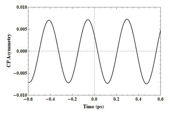
Figure 1. Time dependent CP asymmetry ${\mathcal{A}}_{CP}$(t).

Even though some previous theorists employed QCDF approach [5,18] but the present work is different in several aspects from them. In the present work, the structure of the effective parameters ($a_i^h$) is different from the one of Refs. [5,18]. We also have reported the CP violation which has not been done before for the present decay channel. Finally we include the error analysis of the BR and CP violation calculations. Therefore we think that the reported results in this paper will be helpful for future experiment as well as theoretical studies.

4. Conclusions

In this work, we studied the $\overline{B_s^0}\to \varphi \varphi$ decay mode in the framework of the QCDF approach. In doing this we employed QCDF approach in the NDR scheme at NLO contributions. In this study, we calculated the branching ratio and the $CP$ violation. After numerical evaluation, we found that the BR of $\overline{B_s^0}\to \varphi \varphi$ decay is $(1.56\pm 0.23)\times {10}^{-5}$. This value for $BR$ is consistent with the experimental values as well as with the other theoretically predicted ones. We also calculated the CP violation asymmetries and we found that the present decay mode is governed by the longitudinal amplitude (i.e., for $h=0$). The calculated values for ${\mathcal{A}}_{CP}^{\mathrm{dir}}$, ${\mathcal{A}}_{CP}^{\mathrm{mix}}$ and ${\mathcal{A}}_{CP}^{\Delta \Gamma }$ are $0.00355\pm 0.00152,-0.00629\pm 0.03119$ and $0.99997\pm 0.00019$, respectively. These values are consistent with the available theoretical ones.

References

- Sakarov, A.D. Violation of CP invariance, C asymmetry, and baryon asymmetry of the universe. JETP Lett. 1967, 5, 24–27. [Google Scholar]
- Kobayashi, M.; Maskawa, T. CP-violation in the renormalizable theory of weak interaction. Prog. Theor. Phys. 1973, 49, 652–657. [Google Scholar] [CrossRef]
- Du, D.; Yang, D.; Zhu, G. Analysis of the decays B → ππ and πk with QCD factorization in the heavy quark limit. Phys. Lett. B 2000, 488, 46–54. [Google Scholar] [CrossRef]
- Fleischer, R. Flavour Physics and CP Violation. arXiv 2006, arXiv:hep-ph/0608010. [Google Scholar]
- Beneke, M.; Rohrer, J.; Yang, D. Branching fractions, polarisation and asymmetries of B → VV decays. Nucl. Phys. B 2007, 774, 64–101. [Google Scholar] [CrossRef]
- Abe, K.; Abe, R.; Adachi, I.; Ahn, B.S.; Aihara, H.; Akatsu, M.; Alimonti, G.; Asai, K.; Asai, M.; Asano, Y.; et al. Observation of large CP violation in the neutral B meson system. Phys. Rev. Lett. 2001, 87, 091802. [Google Scholar] [CrossRef]
- Aubert, B.; Boutigny, D.; De Bonis, I.; Gaillard, J.M.; Jeremie, A.; Karyotakis, Y.; Lees, J.P.; Robbe, P.; Tisserand, V.; Palano, A.; et al. Measurement of CP-violating asymmetries in B0 decays to CP eigenstates. Phys. Rev. Lett. 2001, 86, 2515. [Google Scholar] [CrossRef]
- Acosta, D.; Adelman, J.; Affolder, T.; Akimoto, T.; Albrow, M.G.; Ambrose, D.; Amerio, S.; Amidei, D.; Anastassov, A.; Anikeev, K.; et al. Evidence for Decay and Measurements of Branching Ratio and ACP for B+ → ϕK+. Phys. Rev. Lett. 2005, 95, 031801. [Google Scholar] [CrossRef]
- Aaltonen, T.; González, B.Á.; Amerio, S.; Amidei, D.; Anastassov, A.; Annovi, A.; Antos, J.; Apollinari, G.; Appel, J.A.; Apresyan, A.; et al. Measurement of Polarization and Search for CP Violation in Decays. Phys. Rev. Lett. 2011, 107, 261802. [Google Scholar] [CrossRef]
- Aaij, R.; Adeva, B.; Adinolfi, M.; Affolder, A.; Ajaltouni, Z.; Akar, S.; Albrecht, J.; Alessio, F.; Alexander, M.; Ali, S.; et al. (LHCb Collaboration) Measurement of the branching fraction and search for the decay . JHEP 2015, 10, 053. [Google Scholar] [CrossRef]
- Olsen, S.L. Flavor Physics in the LHC Era. arXiv 2014, arXiv:1409.0273. [Google Scholar]
- Li, X.; Lu, G.; Yang, Y.D. Charmless decays in QCD factorization. Phys. Rev. D 2003, 68, 114015, Erratum in 2005, 71, 019902. [Google Scholar] [CrossRef]
- Beneke, M.; Buchalla, G.; Neubert, M.; Sachrajda, C.T. QCD factorization in B → πK,ππ decays and extraction of Wolfenstein parameters. Nucl. Phys. B 2001, 606, 245–321. [Google Scholar] [CrossRef]
- Beneke, M.; Neubert, M. Flavor-singlet B-decay amplitudes in QCD factorization. Nucl. Phys. B 2003, 651, 225–248. [Google Scholar] [CrossRef]
- Beneke, M.; Neubert, M. QCD factorization for B → PP and B → PV decays. Nucl. Phys. B 2003, 675, 333–415. [Google Scholar] [CrossRef]
- Chen, Y.H.; Cheng, H.Y.; Tseng, B.; Yang, K.C. Charmless hadronic two-body decays of Bu and Bd mesons. Phys. Rev. D 1999, 60, 094014. [Google Scholar] [CrossRef]
- Cheng, H.Y.; Yang, K.C. Branching ratios and polarization in B → VV, VA, AA decays. Phys. Rev. D 2008, 78, 094001. [Google Scholar] [CrossRef]
- Cheng, H.Y.; Chua, C.K. QCD factorization for charmless hadronic Bs decays revisited. Phys. Rev. D 2009, 80, 114026. [Google Scholar] [CrossRef]
- Kamal, A.; Khan, H.R.; Alhendi, H.A. Analytic Calculations of the Branching Ratio and CP Violation in Decay. Phys. Atom. Nuclei 2019, 82, 299–308, Erratum in 2019, 82, 549. [Google Scholar] [CrossRef]
- Yan, D.C.; Liu, X.; Xiao, Z.J. Anatomy of Bs → VV decays and effects of next-to-leading order contributions in the perturbative QCD factorization approach. Nucl. Phys. B 2008, 935, 17–39. [Google Scholar] [CrossRef]
- Zou, Z.T.; Ali, A.; Lü, C.D.; Liu, X.; Li, Y. Improved estimates of the Bs → VV decays in perturbative QCD approach. Phys. Rev. D 2015, 91, 054033. [Google Scholar] [CrossRef]
- Bauer, C.W.; Pirjol, D.; Rothstein, I.Z.; Stewart, I.W. B → M1M2: Factorization, charming penguins, strong phases, and polarization. Phys. Rev. D 2004, 70, 054015. [Google Scholar] [CrossRef]
- Wang, C.; Zhou, S.H.; Li, Y.; Lü, C.D. Global analysis of charmless B decays into two vector mesons in soft-collinear effective theory. Phys. Rev. D 2017, 96, 073004. [Google Scholar] [CrossRef]
- Wang, C.; Zhang, Q.A.; Li, Y.; Lü, C.D. Charmless B(s) → VV decays in factorization-assisted topological-amplitude approach. Eur. Phys. J. C 2017, 77, 333. [Google Scholar] [CrossRef]
- Patrignani, C.P.D.G.; Weinberg, D.H.; Woody, C.L.; Chivukula, R.S.; Buchmueller, O.; Kuyanov, Y.V.; Blucher, E.; Willocq, S.; Höcker, A.; Lippmann, C.; et al. Review of particle physics. Chin. Phys. C 2016, 40, 100001. [Google Scholar]
- Buchalla, G.; Buras, A.J.; Lautenbacher, M.E. Weak decays beyond leading logarithms. Rev. Mod. Phys. 1996, 68, 1125. [Google Scholar] [CrossRef]
- Thomson, M. Modern Particle Physics, 1st ed.; Cambridge University Press: Cambridge, UK, 2013; pp. 528–530. ISBN 978-1-107-03426-6. [Google Scholar]
- Datta, A.; London, D. Triple-product correlations in B → VV decays and new physics. Int. J. Mod. Phys. A 2004, 19, 2505–2544. [Google Scholar] [CrossRef]
- Ali, A.; Greub, C. Analysis of two-body nonleptonic B decays involving light mesons in the standard model. Phys. Rev. D 1998, 57, 2996. [Google Scholar] [CrossRef]
- Tanabashi, M.; Hagiwara, K.; Hikasa, K.; Nakamura, K.; Sumino, Y.; Takahashi, F.; Tanaka, J.; Agashe, K.; Aielli, G.; Amsler, C.; et al. Review of particle physics. Phys. Rev. D 2018, 98, 030001. [Google Scholar] [CrossRef]
- Amhis, Y.; Banerjee, S.; Ben-Haim, E.; Bona, M.; Bozek, A.; Bozzi, C.; Brodzicka, J.; Chrzaszcz, M.; Dingfelder, J.; Egede, U.; et al. (HFLAV) Averages of b-hadron, c-hadron and τ-lepton properties as of 2018. arXiv 2019, arXiv:1909.12524. [Google Scholar]
© 2020 by the authors. Licensee MDPI, Basel, Switzerland. This article is an open access article distributed under the terms and conditions of the Creative Commons Attribution (CC BY) license (http://creativecommons.org/licenses/by/4.0/).