
Enhancer-LSTMAtt: A Bi-LSTM and Attention-Based Deep Learning Method for Enhancer Recognition


Abstract
:1. Introduction
2. Data
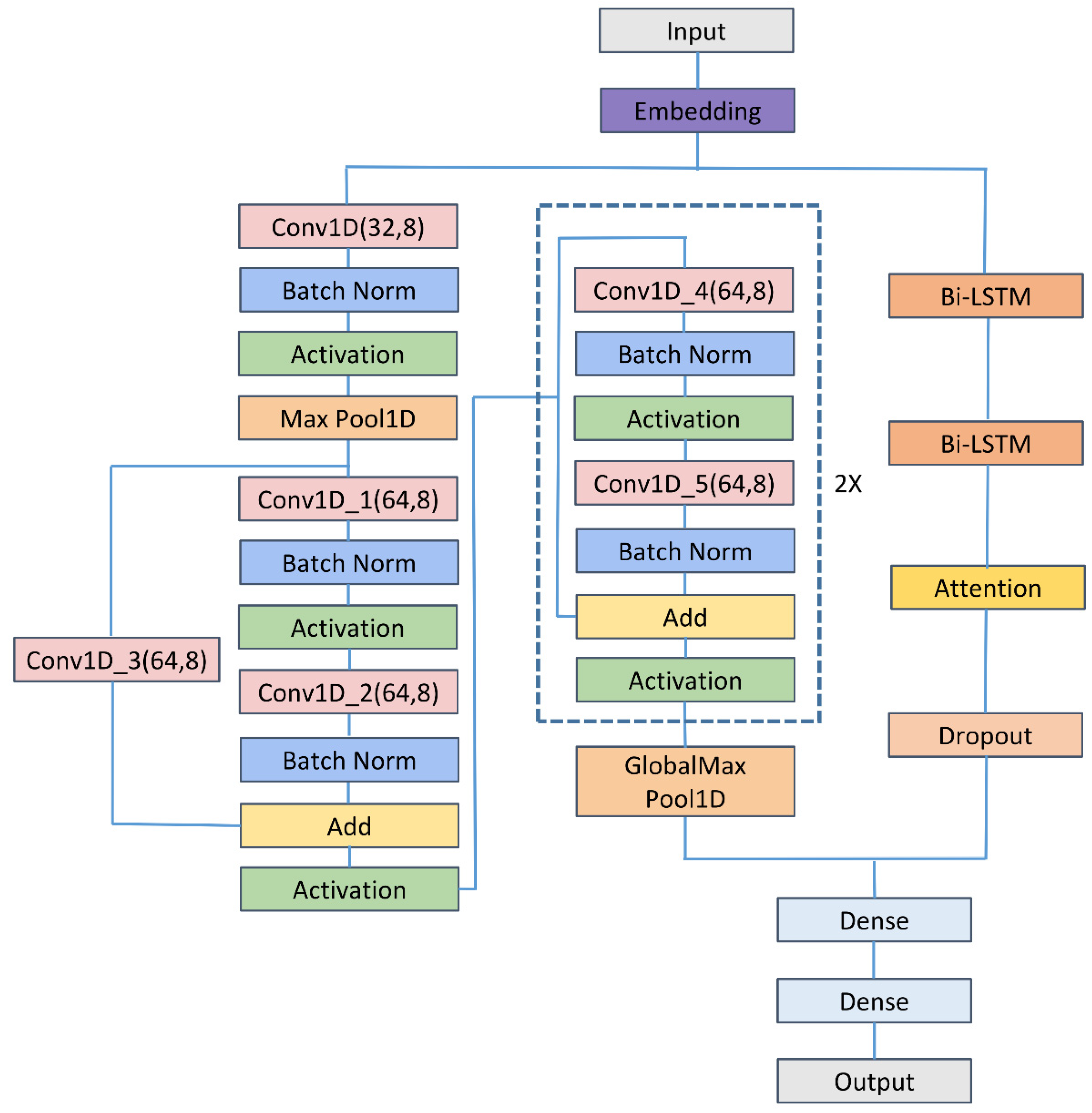
3. Methods
3.1. Embedding Layer
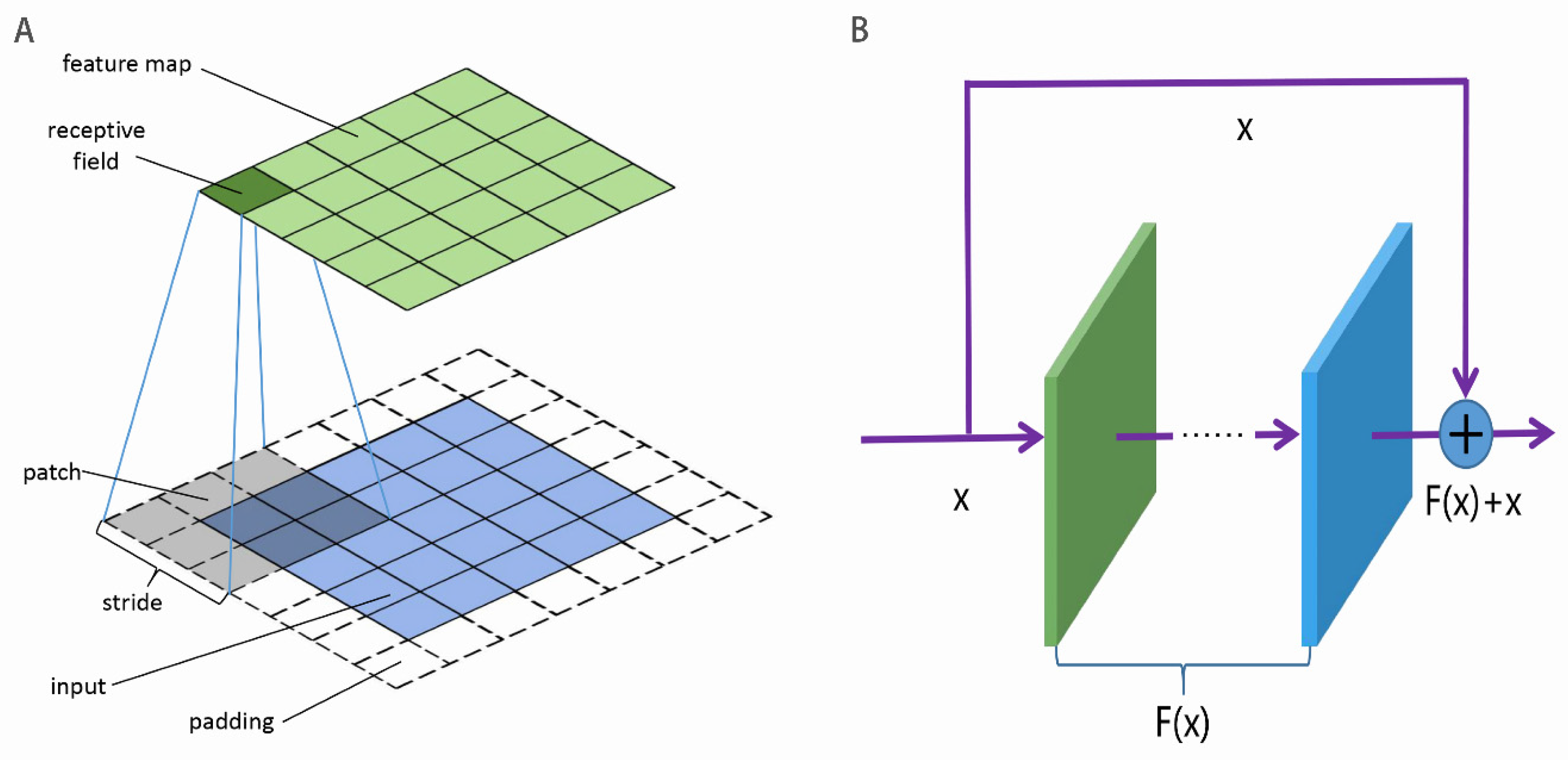
3.2. CNN
3.3. ResNet
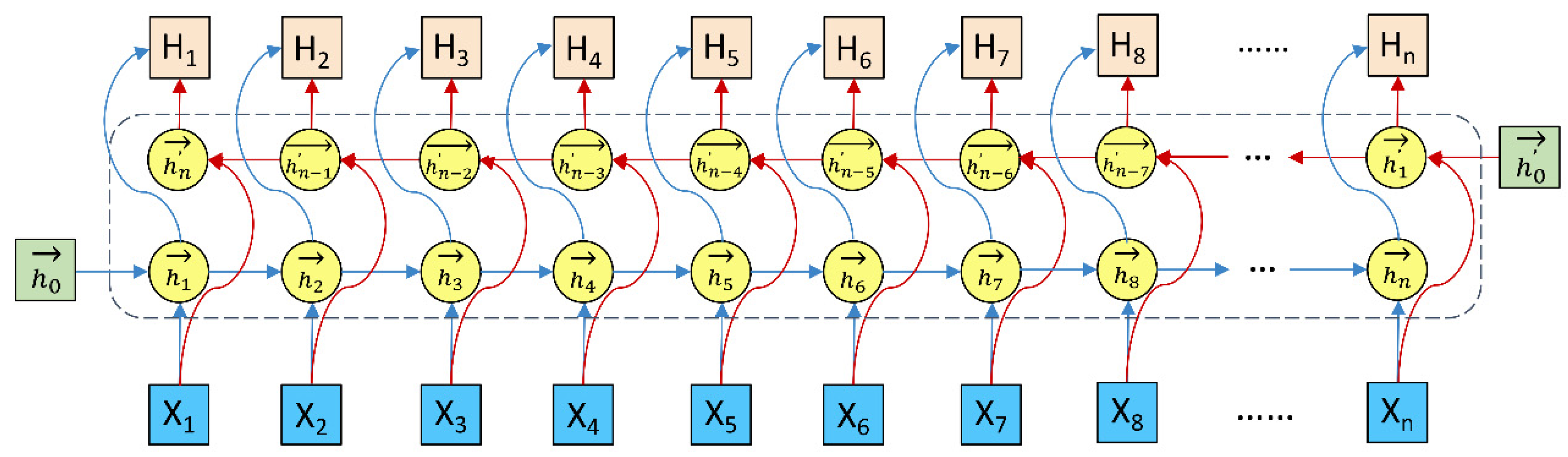
3.4. Bi-LSTM
3.5. Feed-Forward Attention
3.6. Dropout Layer
3.7. Flatten Layer and Fully Connected Layer
4. Cross Validation and Evaluation Metrics
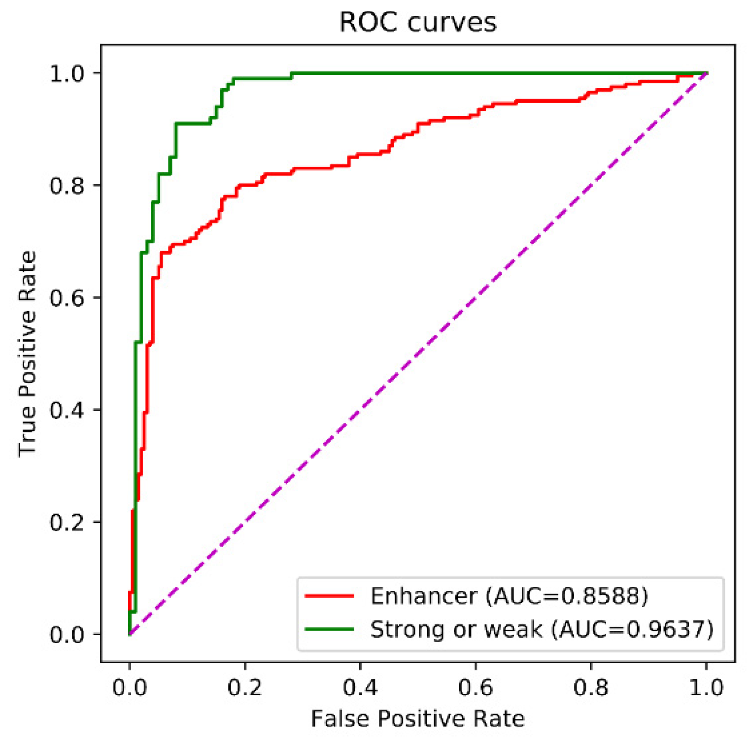
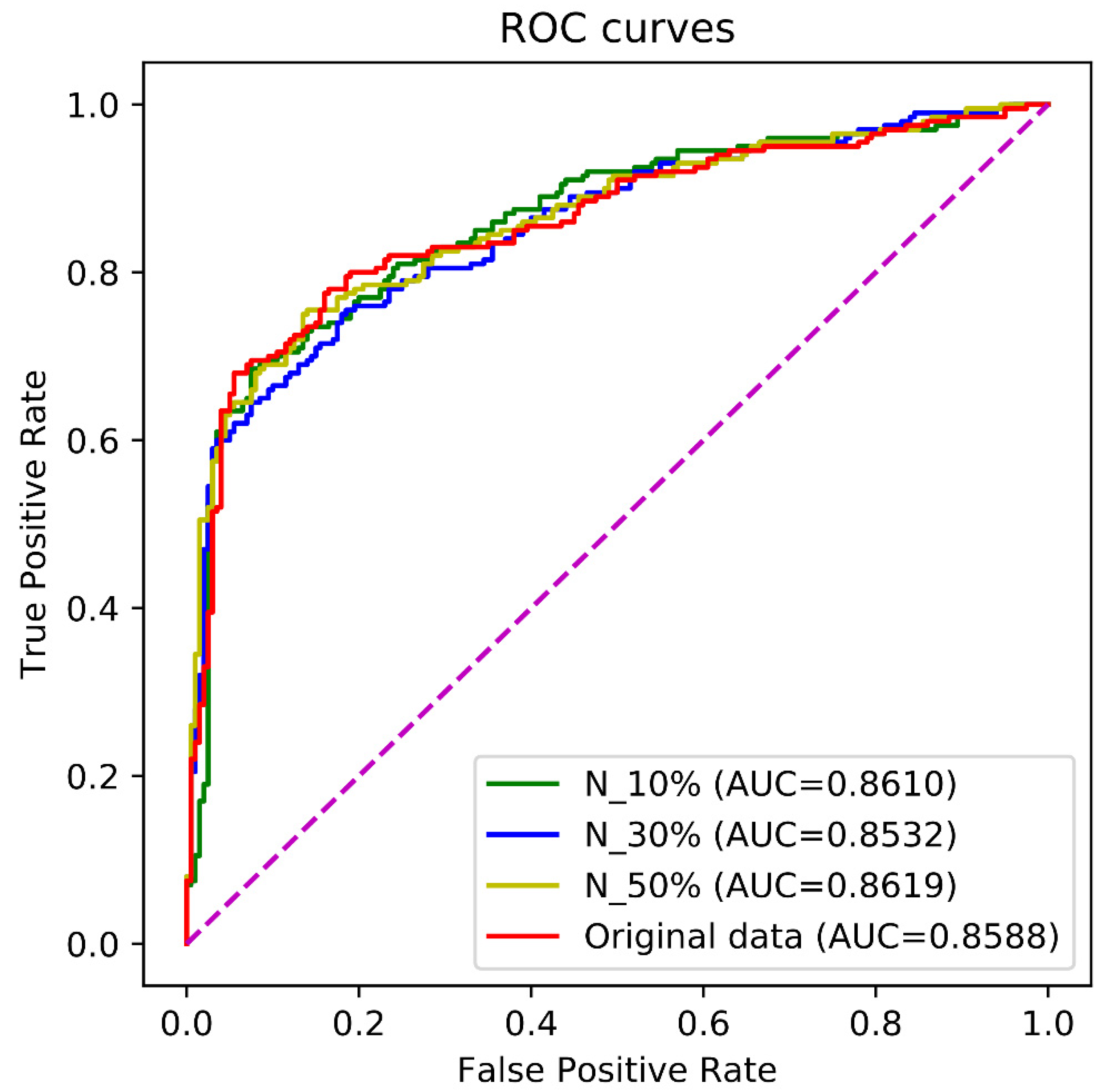
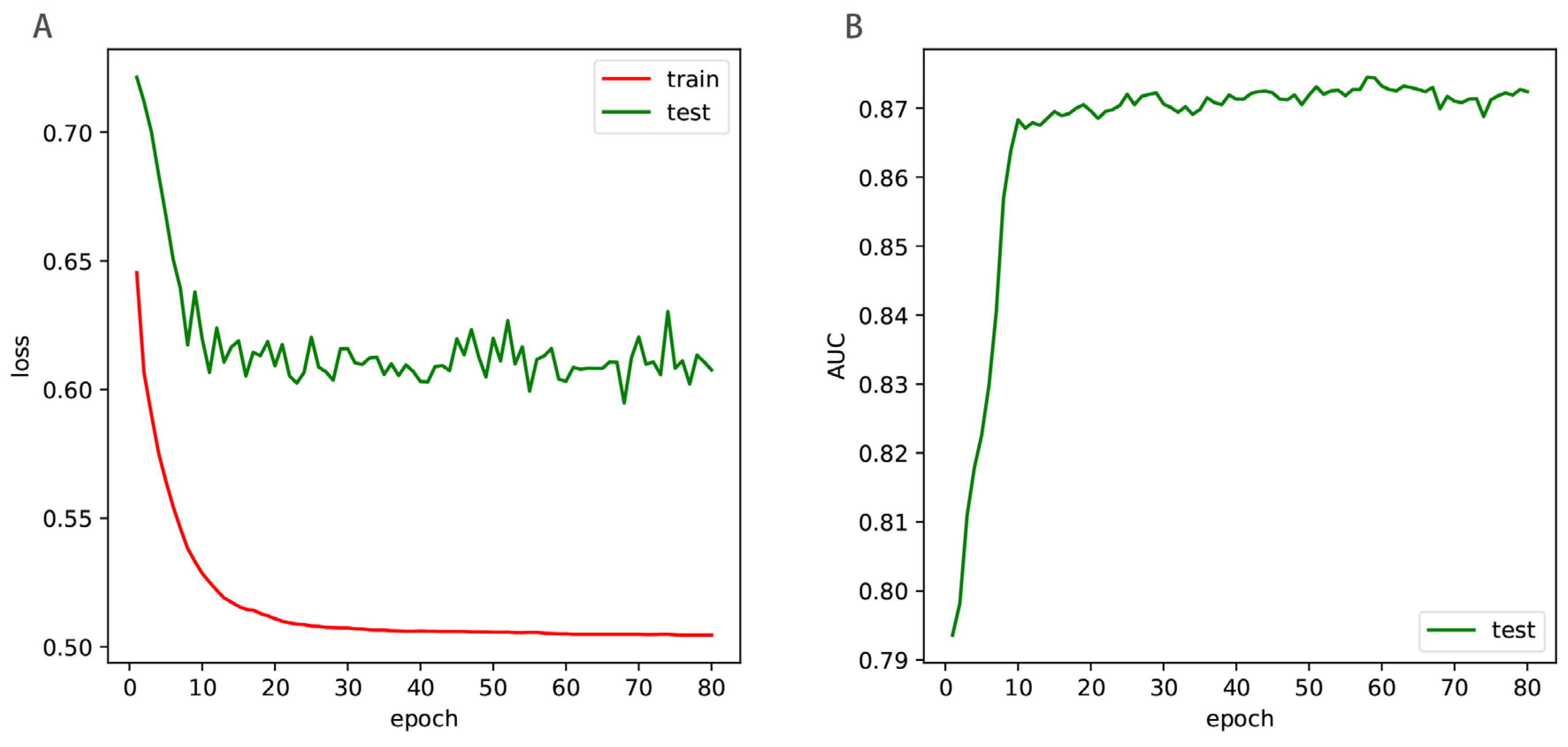
5. Results
5.1. Comparison with State-of-the-Art Methods
5.2. Enhancer-LSTMAtt Webserver
5.3. Discussion
6. Conclusions
Author Contributions
Funding
Institutional Review Board Statement
Informed Consent Statement
Data Availability Statement
Conflicts of Interest
References
- Blackwood, E.M.; Kadonaga, J.T. Going the distance: A current view of enhancer action. Science 1998, 281, 60–63. [Google Scholar] [CrossRef] [PubMed] [Green Version]
- Pennacchio, L.A.; Bickmore, W.; Dean, A.; Nobrega, M.A.; Bejerano, G. Enhancers: Five essential questions. Nat. Rev. Genet. 2013, 14, 288–295. [Google Scholar] [CrossRef] [PubMed]
- Maston, G.A.; Evans, S.K.; Green, M.R. Transcriptional regulatory elements in the human genome. Annu. Rev. Genom. Hum. Genet. 2006, 7, 29–59. [Google Scholar] [CrossRef] [PubMed] [Green Version]
- Grosveld, F.; van Staalduinen, J.; Stadhouders, R. Transcriptional Regulation by (Super) Enhancers: From Discovery to Mechanisms. Annu. Rev. Genom. Hum. Genet. 2021, 22, 127–146. [Google Scholar] [CrossRef] [PubMed]
- Shlyueva, D.; Stampfel, G.; Stark, A. Transcriptional enhancers: From properties to genome-wide predictions. Nat. Rev. Genet. 2014, 15, 272–286. [Google Scholar] [CrossRef] [PubMed]
- Parker, S.C.; Stitzel, M.L.; Taylor, D.L.; Orozco, J.M.; Erdos, M.R.; Akiyama, J.A.; van Bueren, K.L.; Chines, P.S.; Narisu, N.; Black, B.L. Chromatin stretch enhancer states drive cell-specific gene regulation and harbor human disease risk variants. Proc. Natl. Acad. Sci. USA 2013, 110, 17921–17926. [Google Scholar] [CrossRef] [Green Version]
- Schoenfelder, S.; Fraser, P. Long-range enhancer–promoter contacts in gene expression control. Nat. Rev. Genet. 2019, 20, 437–455. [Google Scholar] [CrossRef]
- Chan, Y.F.; Marks, M.E.; Jones, F.C.; Villarreal, G.; Shapiro, M.D.; Brady, S.D.; Southwick, A.M.; Absher, D.M.; Grimwood, J.; Schmutz, J. Adaptive evolution of pelvic reduction in sticklebacks by recurrent deletion of a Pitx1 enhancer. Science 2010, 327, 302–305. [Google Scholar] [CrossRef] [Green Version]
- Levine, M. Transcriptional enhancers in animal development and evolution. Curr. Biol. 2010, 20, R754–R763. [Google Scholar] [CrossRef] [Green Version]
- Bonn, S.; Zinzen, R.P.; Girardot, C.; Gustafson, E.H.; Perez-Gonzalez, A.; Delhomme, N.; Ghavi-Helm, Y.; Wilczyński, B.; Riddell, A.; Furlong, E.E. Tissue-specific analysis of chromatin state identifies temporal signatures of enhancer activity during embryonic development. Nat. Genet. 2012, 44, 148–156. [Google Scholar] [CrossRef]
- Heintzman, N.D.; Hon, G.C.; Hawkins, R.D.; Kheradpour, P.; Stark, A.; Harp, L.F.; Ye, Z.; Lee, L.K.; Stuart, R.K.; Ching, C.W. Histone modifications at human enhancers reflect global cell-type-specific gene expression. Nature 2009, 459, 108–112. [Google Scholar] [CrossRef] [PubMed] [Green Version]
- Visel, A.; Blow, M.J.; Li, Z.; Zhang, T.; Akiyama, J.A.; Holt, A.; Plajzer-Frick, I.; Shoukry, M.; Wright, C.; Chen, F. ChIP-seq accurately predicts tissue-specific activity of enhancers. Nature 2009, 457, 854–858. [Google Scholar] [CrossRef] [Green Version]
- Heintzman, N.D.; Stuart, R.K.; Hon, G.; Fu, Y.; Ching, C.W.; Hawkins, R.D.; Barrera, L.O.; Van Calcar, S.; Qu, C.; Ching, K.A. Distinct and predictive chromatin signatures of transcriptional promoters and enhancers in the human genome. Nat. Genet. 2007, 39, 311–318. [Google Scholar] [CrossRef]
- Jin, F.; Li, Y.; Ren, B.; Natarajan, R. PU. 1 and C/EBPα synergistically program distinct response to NF-κB activation through establishing monocyte specific enhancers. Proc. Natl. Acad. Sci. USA 2011, 108, 5290–5295. [Google Scholar] [CrossRef] [PubMed] [Green Version]
- Kim, T.-K.; Hemberg, M.; Gray, J.M.; Costa, A.M.; Bear, D.M.; Wu, J.; Harmin, D.A.; Laptewicz, M.; Barbara-Haley, K.; Kuersten, S. Widespread transcription at neuronal activity-regulated enhancers. Nature 2010, 465, 182–187. [Google Scholar] [CrossRef] [PubMed] [Green Version]
- Rajagopal, N.; Xie, W.; Li, Y.; Wagner, U.; Wang, W.; Stamatoyannopoulos, J.; Ernst, J.; Kellis, M.; Ren, B. RFECS: A random-forest based algorithm for enhancer identification from chromatin state. PLoS Comput. Biol. 2013, 9, e1002968. [Google Scholar] [CrossRef]
- Whyte, W.A.; Orlando, D.A.; Hnisz, D.; Abraham, B.J.; Lin, C.Y.; Kagey, M.H.; Rahl, P.B.; Lee, T.I.; Young, R.A. Master transcription factors and mediator establish super-enhancers at key cell identity genes. Cell 2013, 153, 307–319. [Google Scholar] [CrossRef] [Green Version]
- Kleftogiannis, D.; Kalnis, P.; Bajic, V.B. Progress and challenges in bioinformatics approaches for enhancer identification. Brief. Bioinform. 2016, 17, 967–979. [Google Scholar] [CrossRef] [Green Version]
- Johnson, D.S.; Mortazavi, A.; Myers, R.M.; Wold, B. Genome-wide mapping of in vivo protein-DNA interactions. Science 2007, 316, 1497–1502. [Google Scholar] [CrossRef] [Green Version]
- Robertson, G.; Hirst, M.; Bainbridge, M.; Bilenky, M.; Zhao, Y.; Zeng, T.; Euskirchen, G.; Bernier, B.; Varhol, R.; Delaney, A. Genome-wide profiles of STAT1 DNA association using chromatin immunoprecipitation and massively parallel sequencing. Nat. Methods 2007, 4, 651–657. [Google Scholar] [CrossRef]
- Bulyk, M.L.; Gentalen, E.; Lockhart, D.J.; Church, G.M. Quantifying DNA–protein interactions by double-stranded DNA arrays. Nat. Biotechnol. 1999, 17, 573–577. [Google Scholar] [CrossRef] [PubMed]
- Tuerk, C.; Gold, L. Systematic evolution of ligands by exponential enrichment: RNA ligands to bacteriophage T4 DNA polymerase. Science 1990, 249, 505–510. [Google Scholar] [CrossRef]
- Li, J.J.; Herskowitz, I. Isolation of ORC6, a component of the yeast origin recognition complex by a one-hybrid system. Science 1993, 262, 1870–1874. [Google Scholar] [CrossRef] [PubMed]
- Meng, X.; Brodsky, M.H.; Wolfe, S.A. A bacterial one-hybrid system for determining the DNA-binding specificity of transcription factors. Nat. Biotechnol. 2005, 23, 988–994. [Google Scholar] [CrossRef] [PubMed] [Green Version]
- Heintzman, N.D.; Ren, B. Finding distal regulatory elements in the human genome. Curr. Opin. Genet. Dev. 2009, 19, 541–549. [Google Scholar] [CrossRef] [Green Version]
- May, D.; Blow, M.J.; Kaplan, T.; McCulley, D.J.; Jensen, B.C.; Akiyama, J.A.; Holt, A.; Plajzer-Frick, I.; Shoukry, M.; Wright, C. Large-scale discovery of enhancers from human heart tissue. Nat. Genet. 2012, 44, 89–93. [Google Scholar] [CrossRef] [PubMed]
- Boyle, A.P.; Song, L.; Lee, B.-K.; London, D.; Keefe, D.; Birney, E.; Iyer, V.R.; Crawford, G.E.; Furey, T.S. High-resolution genome-wide in vivo footprinting of diverse transcription factors in human cells. Genome Res. 2011, 21, 456–464. [Google Scholar] [CrossRef] [PubMed] [Green Version]
- Boyle, A.P.; Davis, S.; Shulha, H.P.; Meltzer, P.; Margulies, E.H.; Weng, Z.; Furey, T.S.; Crawford, G.E. High-resolution mapping and characterization of open chromatin across the genome. Cell 2008, 132, 311–322. [Google Scholar] [CrossRef] [Green Version]
- Consortium, E.P. Identification and analysis of functional elements in 1% of the human genome by the ENCODE pilot project. Nature 2007, 447, 799. [Google Scholar] [CrossRef] [Green Version]
- Visel, A.; Bristow, J.; Pennacchio, L.A. Enhancer identification through comparative genomics. Proc. Semin. Cell Dev. Biol. 2007, 18, 140–152. [Google Scholar] [CrossRef] [Green Version]
- Won, K.-J.; Zhang, X.; Wang, T.; Ding, B.; Raha, D.; Snyder, M.; Ren, B.; Wang, W. Comparative annotation of functional regions in the human genome using epigenomic data. Nucleic Acids Res. 2013, 41, 4423–4432. [Google Scholar] [CrossRef] [PubMed]
- Ghandi, M.; Lee, D.; Mohammad-Noori, M.; Beer, M.A. Enhanced regulatory sequence prediction using gapped k-mer features. PLoS Comput. Biol. 2014, 10, e1003711. [Google Scholar] [CrossRef] [PubMed] [Green Version]
- Min, X.; Zeng, W.; Chen, S.; Chen, N.; Chen, T.; Jiang, R. Predicting enhancers with deep convolutional neural networks. BMC Bioinform. 2017, 18, 35–46. [Google Scholar] [CrossRef] [Green Version]
- Yang, B.; Liu, F.; Ren, C.; Ouyang, Z.; Xie, Z.; Bo, X.; Shu, W. BiRen: Predicting enhancers with a deep-learning-based model using the DNA sequence alone. Bioinformatics 2017, 33, 1930–1936. [Google Scholar] [CrossRef] [Green Version]
- Firpi, H.A.; Ucar, D.; Tan, K. Discover regulatory DNA elements using chromatin signatures and artificial neural network. Bioinformatics 2010, 26, 1579–1586. [Google Scholar] [CrossRef] [PubMed] [Green Version]
- Fernandez, M.; Miranda-Saavedra, D. Genome-wide enhancer prediction from epigenetic signatures using genetic algorithm-optimized support vector machines. Nucleic Acids Res. 2012, 40, e77. [Google Scholar] [CrossRef] [Green Version]
- Erwin, G.D.; Oksenberg, N.; Truty, R.M.; Kostka, D.; Murphy, K.K.; Ahituv, N.; Pollard, K.S.; Capra, J.A. Integrating diverse datasets improves developmental enhancer prediction. PLoS Comput. Biol. 2014, 10, e1003677. [Google Scholar] [CrossRef] [Green Version]
- Kleftogiannis, D.; Kalnis, P.; Bajic, V.B. DEEP: A general computational framework for predicting enhancers. Nucleic Acids Res. 2015, 43, e6. [Google Scholar] [CrossRef] [Green Version]
- Lu, Y.; Qu, W.; Shan, G.; Zhang, C. DELTA: A distal enhancer locating tool based on AdaBoost algorithm and shape features of chromatin modifications. PLoS ONE 2015, 10, e0130622. [Google Scholar] [CrossRef]
- Liu, B.; Fang, L.; Long, R.; Lan, X.; Chou, K.-C. iEnhancer-2L: A two-layer predictor for identifying enhancers and their strength by pseudo k-tuple nucleotide composition. Bioinformatics 2016, 32, 362–369. [Google Scholar] [CrossRef] [Green Version]
- Liu, B. iEnhancer-PsedeKNC: Identification of enhancers and their subgroups based on Pseudo degenerate kmer nucleotide composition. Neurocomputing 2016, 217, 46–52. [Google Scholar] [CrossRef]
- Jia, C.; He, W. EnhancerPred: A predictor for discovering enhancers based on the combination and selection of multiple features. Sci. Rep. 2016, 6, 38741. [Google Scholar] [CrossRef] [Green Version]
- He, W.; Jia, C. EnhancerPred2. 0: Predicting enhancers and their strength based on position-specific trinucleotide propensity and electron–ion interaction potential feature selection. Mol. Biosyst. 2017, 13, 767–774. [Google Scholar] [CrossRef] [PubMed]
- Tahir, M.; Hayat, M.; Kabir, M. Sequence based predictor for discrimination of enhancer and their types by applying general form of Chou’s trinucleotide composition. Comput. Methods Programs Biomed. 2017, 146, 69–75. [Google Scholar] [CrossRef] [PubMed]
- Tahir, M.; Hayat, M.; Khan, S.A. A two-layer computational model for discrimination of enhancer and their types using hybrid features pace of pseudo K-tuple nucleotide composition. Arab. J. Sci. Eng. 2018, 43, 6719–6727. [Google Scholar] [CrossRef]
- Liu, B.; Li, K.; Huang, D.-S.; Chou, K.-C. iEnhancer-EL: Identifying enhancers and their strength with ensemble learning approach. Bioinformatics 2018, 34, 3835–3842. [Google Scholar] [CrossRef]
- Le, N.Q.K.; Yapp, E.K.Y.; Ho, Q.-T.; Nagasundaram, N.; Ou, Y.-Y.; Yeh, H.-Y. iEnhancer-5Step: Identifying enhancers using hidden information of DNA sequences via Chou’s 5-step rule and word embedding. Anal. Biochem. 2019, 571, 53–61. [Google Scholar] [CrossRef]
- Tan, K.K.; Le, N.Q.K.; Yeh, H.-Y.; Chua, M.C.H. Ensemble of deep recurrent neural networks for identifying enhancers via dinucleotide physicochemical properties. Cells 2019, 8, 767. [Google Scholar] [CrossRef] [Green Version]
- Zhang, T.-H.; Flores, M.; Huang, Y. ES-ARCNN: Predicting enhancer strength by using data augmentation and residual convolutional neural network. Anal. Biochem. 2021, 618, 114120. [Google Scholar] [CrossRef]
- Nguyen, Q.H.; Nguyen-Vo, T.-H.; Le, N.Q.K.; Do, T.T.; Rahardja, S.; Nguyen, B.P. iEnhancer-ECNN: Identifying enhancers and their strength using ensembles of convolutional neural networks. BMC Genom. 2019, 20, 951. [Google Scholar] [CrossRef]
- Butt, A.H.; Alkhalaf, S.; Iqbal, S.; Khan, Y.D. EnhancerP-2L: A Gene regulatory site identification tool for DNA enhancer region using CREs motifs. bioRxiv 2020. [Google Scholar] [CrossRef]
- Khanal, J.; Tayara, H.; Chong, K.T. Identifying enhancers and their strength by the integration of word embedding and convolution neural network. IEEE Access 2020, 8, 58369–58376. [Google Scholar] [CrossRef]
- Cai, L.; Ren, X.; Fu, X.; Peng, L.; Gao, M.; Zeng, X. iEnhancer-XG: Interpretable sequence-based enhancers and their strength predictor. Bioinformatics 2021, 37, 1060–1067. [Google Scholar] [CrossRef] [PubMed]
- Li, Q.; Xu, L.; Li, Q.; Zhang, L. Identification and classification of enhancers using dimension reduction technique and recurrent neural network. Comput. Math. Methods Med. 2020, 2020, 8852258. [Google Scholar] [CrossRef] [PubMed]
- Le, N.Q.K.; Ho, Q.-T.; Nguyen, T.-T.-D.; Ou, Y.-Y. A transformer architecture based on BERT and 2D convolutional neural network to identify DNA enhancers from sequence information. Brief. Bioinform. 2021, 22, bbab005. [Google Scholar] [CrossRef]
- Lyu, Y.; Zhang, Z.; Li, J.; He, W.; Ding, Y.; Guo, F. iEnhancer-KL: A novel two-layer predictor for identifying enhancer by position specific of nucleotide composition. IEEE/ACM Trans. Comput. Biol. Bioinform. 2021, 18, 2809–2815. [Google Scholar] [CrossRef]
- Lim, D.Y.; Khanal, J.; Tayara, H.; Chong, K.T. iEnhancer-RF: Identifying enhancers and their strength by enhanced feature representation using random forest. Chemom. Intell. Lab. Syst. 2021, 212, 104284. [Google Scholar] [CrossRef]
- Mu, X.; Wang, Y.; Duan, M.; Liu, S.; Li, F.; Wang, X.; Zhang, K.; Huang, L.; Zhou, F. A Novel Position-Specific Encoding Algorithm (SeqPose) of Nucleotide Sequences and Its Application for Detecting Enhancers. Int. J. Mol. Sci. 2021, 22, 3079. [Google Scholar] [CrossRef]
- Niu, K.; Luo, X.; Zhang, S.; Teng, Z.; Zhang, T.; Zhao, Y. iEnhancer-EBLSTM: Identifying Enhancers and Strengths by Ensembles of Bidirectional Long Short-Term Memory. Front. Genet. 2021, 12, 385. [Google Scholar] [CrossRef]
- Yang, R.; Wu, F.; Zhang, C.; Zhang, L. iEnhancer-GAN: A Deep Learning Framework in Combination with Word Embedding and Sequence Generative Adversarial Net to Identify Enhancers and Their Strength. Int. J. Mol. Sci. 2021, 22, 3589. [Google Scholar] [CrossRef]
- Khan, Z.U.; Pi, D.; Yao, S.; Nawaz, A.; Ali, F.; Ali, S. piEnPred: A bi-layered discriminative model for enhancers and their subtypes via novel cascade multi-level subset feature selection algorithm. Front. Comput. Sci. 2021, 15, 156904. [Google Scholar] [CrossRef]
- Yang, H.; Wang, S.; Xia, X. iEnhancer-RD: Identification of enhancers and their strength using RKPK features and deep neural networks. Anal. Biochem. 2021, 630, 114318. [Google Scholar] [CrossRef] [PubMed]
- Liang, Y.; Zhang, S.; Qiao, H.; Cheng, Y. iEnhancer-MFGBDT: Identifying enhancers and their strength by fusing multiple features and gradient boosting decision tree. Math. Biosci. Eng. 2021, 18, 8797–8814. [Google Scholar] [CrossRef] [PubMed]
- Jumper, J.; Evans, R.; Pritzel, A.; Green, T.; Figurnov, M.; Ronneberger, O.; Tunyasuvunakool, K.; Bates, R.; Žídek, A.; Potapenko, A. Highly accurate protein structure prediction with AlphaFold. Nature 2021, 596, 583–589. [Google Scholar] [CrossRef] [PubMed]
- Baek, M.; DiMaio, F.; Anishchenko, I.; Dauparas, J.; Ovchinnikov, S.; Lee, G.R.; Wang, J.; Cong, Q.; Kinch, L.N.; Schaeffer, R.D. Accurate prediction of protein structures and interactions using a 3-track network. bioRxiv 2021. [Google Scholar] [CrossRef]
- Yu, L.; Zhang, W.; Wang, J.; Yu, Y. Seqgan: Sequence generative adversarial nets with policy gradient. In Proceedings of the AAAI Conference on Artificial Intelligence, San Francisco, CL, USA, 4–9 February 2017. [Google Scholar]
- LeCun, Y.; Boser, B.; Denker, J.; Henderson, D.; Howard, R.; Hubbard, W.; Jackel, L. Handwritten digit recognition with a back-propagation network. Adv. Neural Inf. Process. Syst. 1989, 2, 396–404. [Google Scholar]
- Devlin, J.; Chang, M.-W.; Lee, K.; Toutanova, K. Bert: Pre-training of deep bidirectional transformers for language understanding. arXiv 2018. [Google Scholar] [CrossRef]
- Ernst, J.; Kheradpour, P.; Mikkelsen, T.S.; Shoresh, N.; Ward, L.D.; Epstein, C.B.; Zhang, X.; Wang, L.; Issner, R.; Coyne, M. Mapping and analysis of chromatin state dynamics in nine human cell types. Nature 2011, 473, 43–49. [Google Scholar] [CrossRef]
- Ernst, J.; Kellis, M. ChromHMM: Automating chromatin-state discovery and characterization. Nat. Methods 2012, 9, 215–216. [Google Scholar] [CrossRef] [Green Version]
- Li, W.; Godzik, A. Cd-hit: A fast program for clustering and comparing large sets of protein or nucleotide sequences. Bioinformatics 2006, 22, 1658–1659. [Google Scholar] [CrossRef] [Green Version]
- Fu, L.; Niu, B.; Zhu, Z.; Wu, S.; Li, W. CD-HIT: Accelerated for clustering the next-generation sequencing data. Bioinformatics 2012, 28, 3150–3152. [Google Scholar] [CrossRef]
- Huang, Y.; Niu, B.; Gao, Y.; Fu, L.; Li, W. CD-HIT Suite: A web server for clustering and comparing biological sequences. Bioinformatics 2010, 26, 680–682. [Google Scholar] [CrossRef] [PubMed]
- Huang, G.; Zeng, W. A discrete hidden Markov model for detecting histone crotonyllysine sites. Match Commun. Math. Comput. Chem. 2016, 75, 717–730. [Google Scholar]
- Puton, T.; Kozlowski, L.; Tuszynska, I.; Rother, K.; Bujnicki, J.M. Computational methods for prediction of protein–RNA interactions. J. Struct. Biol. 2012, 179, 261–268. [Google Scholar] [CrossRef] [PubMed]
- Huang, G.; Chu, C.; Huang, T.; Kong, X.; Zhang, Y.; Zhang, N.; Cai, Y.-D. Exploring mouse protein function via multiple approaches. PLoS ONE 2016, 11, e0166580. [Google Scholar] [CrossRef] [Green Version]
- Huang, G.; Zheng, Y.; Wu, Y.-Q.; Han, G.-S.; Yu, Z.-G. An information entropy-based approach for computationally identifying histone lysine butyrylation. Front. Genet. 2020, 10, 1325. [Google Scholar] [CrossRef]
- Liu, K.; Cao, L.; Du, P.; Chen, W. im6A-TS-CNN: Identifying the N6-methyladenine site in multiple tissues by using the convolutional neural network. Mol. Ther. Nucleic Acids 2020, 21, 1044–1049. [Google Scholar] [CrossRef]
- Fang, T.; Zhang, Z.; Sun, R.; Zhu, L.; He, J.; Huang, B.; Xiong, Y.; Zhu, X. RNAm5CPred: Prediction of RNA 5-methylcytosine sites based on three different kinds of nucleotide composition. Mol. Ther.-Nucleic Acids 2019, 18, 739–747. [Google Scholar] [CrossRef] [Green Version]
- Li, J.; Li, H.; Ye, X.; Zhang, L.; Xu, Q.; Ping, Y.; Jing, X.; Jiang, W.; Liao, Q.; Liu, B. IIMLP: Integrated information-entropy-based method for LncRNA prediction. BMC Bioinform. 2021, 22, 243. [Google Scholar] [CrossRef]
- He, K.; Zhang, X.; Ren, S.; Sun, J. Deep residual learning for image recognition. In Proceedings of the IEEE Conference on Computer Vision and Pattern Recognition, Las Vegas, NV, USA, 27–30 June 2016; pp. 770–778. [Google Scholar]
- Targ, S.; Almeida, D.; Lyman, K. Resnet in resnet: Generalizing residual architectures. arXiv 2016. [Google Scholar] [CrossRef]
- Li, S.; Jiao, J.; Han, Y.; Weissman, T. Demystifying resnet. arXiv 2016. [Google Scholar] [CrossRef]
- Siami-Namini, S.; Tavakoli, N.; Namin, A.S. The performance of LSTM and BiLSTM in forecasting time series. In Proceedings of the 2019 IEEE International Conference on Big Data (Big Data), Los Angeles, CA, USA, 9–12 December 2019; pp. 3285–3292. [Google Scholar]
- Kiperwasser, E.; Goldberg, Y. Simple and accurate dependency parsing using bidirectional LSTM feature representations. Trans. Assoc. Comput. Linguist. 2016, 4, 313–327. [Google Scholar] [CrossRef]
- Liu, G.; Guo, J. Bidirectional LSTM with attention mechanism and convolutional layer for text classification. Neurocomputing 2019, 337, 325–338. [Google Scholar] [CrossRef]
- Hong, Z.; Zeng, X.; Wei, L.; Liu, X. Identifying enhancer–promoter interactions with neural network based on pre-trained DNA vectors and attention mechanism. Bioinformatics 2020, 36, 1037–1043. [Google Scholar] [CrossRef] [PubMed]
- Neishi, M.; Sakuma, J.; Tohda, S.; Ishiwatari, S.; Yoshinaga, N.; Toyoda, M. A bag of useful tricks for practical neural machine translation: Embedding layer initialization and large batch size. In Proceedings of the 4th Workshop on Asian Translation (WAT2017), Taipei, Taiwan, 27 November 2017; pp. 99–109. [Google Scholar]
- Allen-Zhu, Z.; Li, Y.; Song, Z. A convergence theory for deep learning via over-parameterization. In Proceedings of the International Conference on Machine Learning, Long Beach, CA, USA, 10–15 June 2019; pp. 242–252. [Google Scholar]
- Hochreiter, S.; Schmidhuber, J. Long short-term memory. Neural Comput. 1997, 9, 1735–1780. [Google Scholar] [CrossRef]
- Pearlmutter, B.A. Learning state space trajectories in recurrent neural networks. Neural Comput. 1989, 1, 263–269. [Google Scholar] [CrossRef]
- Giles, C.L.; Kuhn, G.M.; Williams, R.J. Dynamic recurrent neural networks: Theory and applications. IEEE Trans. Neural Netw. 1994, 5, 153–156. [Google Scholar] [CrossRef]
- Sak, H.; Senior, A.; Rao, K.; Beaufays, F. Fast and accurate recurrent neural network acoustic models for speech recognition. arXiv 2015. [Google Scholar] [CrossRef]
- Saha, S.; Raghava, G.P.S. Prediction of continuous B-cell epitopes in an antigen using recurrent neural network. Proteins: Struct. Funct. Bioinform. 2006, 65, 40–48. [Google Scholar] [CrossRef]
- Arras, L.; Montavon, G.; Müller, K.-R.; Samek, W. Explaining recurrent neural network predictions in sentiment analysis. arXiv 2017. [Google Scholar] [CrossRef]
- Du, Y.; Wang, W.; Wang, L. Hierarchical recurrent neural network for skeleton based action recognition. In Proceedings of the IEEE Conference on Computer Vision and Pattern Recognition, Boston, MA, USA, 7–12 June 2015; pp. 1110–1118. [Google Scholar]
- Medsker, L.R.; Jain, L. Recurrent neural networks. Des. Appl. 2001, 5, 64–67. [Google Scholar]
- Schuster, M.; Paliwal, K.K. Bidirectional recurrent neural networks. IEEE Trans. Signal Process. 1997, 45, 2673–2681. [Google Scholar] [CrossRef] [Green Version]
- Raffel, C.; Ellis, D.P. Feed-forward networks with attention can solve some long-term memory problems. arXiv 2015. [Google Scholar] [CrossRef]
- Vaswani, A.; Shazeer, N.; Parmar, N.; Uszkoreit, J.; Jones, L.; Gomez, A.N.; Kaiser, Ł.; Polosukhin, I. Attention is all you need. In Proceedings of the Advances in Neural Information Processing Systems, Long Beach, CA, USA, 4–9 December 2017; pp. 5998–6008. [Google Scholar]
- Hinton, G.E.; Srivastava, N.; Krizhevsky, A.; Sutskever, I.; Salakhutdinov, R.R. Improving neural networks by preventing co-adaptation of feature detectors. arXiv 2012. [Google Scholar] [CrossRef]
- Baldi, P.; Sadowski, P.J. Understanding dropout. Adv. Neural Inf. Processing Syst. 2013, 26, 2814–2822. [Google Scholar]


| Layers | Shape of Output | Number of Parameters |
|---|---|---|
| Input | (None, 200) | 0 |
| Embedding | (None, 200, 32) | 160 |
| Conv1D(32, 8) | (None, 200, 32) | 8224 |
| Batch Normalization | (None, 200, 32) | 128 |
| Activation | (None, 200, 32) | 0 |
| Max Pooling | (None, 199, 32) | 0 |
| Conv1D_1(64, 8) | (None, 96, 64) | 16,448 |
| Batch Normalization | (None, 96, 64) | 256 |
| Activation | (None, 96, 64) | 0 |
| Conv1D_2(64, 8) | (None, 96, 64) | 32,832 |
| Batch Normalization | (None, 96, 64) | 256 |
| Conv1D_3(64, 8) | (None, 96, 64) | 16,448 |
| Add | (None, 96, 64) | 0 |
| Activation | (None, 96, 64) | 0 |
| Conv1D_4(64, 8) | (None, 96, 64) | 32,832 |
| Batch Normalization | (None, 96, 64) | 256 |
| Activation | (None, 96, 64) | 0 |
| Conv1D_5(64, 8) | (None, 96, 64) | 32,832 |
| Batch Normalization | (None, 96, 64) | 256 |
| Add | (None, 96, 64) | 0 |
| Activation | (None, 96, 64) | 0 |
| Conv1D_6(64, 8) | (None, 96, 64) | 32,832 |
| Batch Normalization | (None, 96, 64) | 256 |
| Activation | (None, 96, 64) | 0 |
| Conv1D_7(64, 8) | (None, 96, 64) | 32,832 |
| Batch Normalization | (None, 96, 64) | 256 |
| Add | (None, 96, 64) | 0 |
| Activation | (None, 96, 64) | 0 |
| Global Max Pooling | (None, 64) | 0 |
| Bidirectional LSTM | (None, 200, 64) | 16,640 |
| Bidirectional LSTM | (None, 200, 64) | 24,832 |
| Attention | (None, 64) | 264 |
| Dropout | (None, 64) | 0 |
| Concatenate | (None, 128) | 0 |
| Dense(16) | (None, 16) | 2064 |
| Dense(1) | (None, 1) | 17 |
| SN | SP | ACC | MCC | AUC | |
|---|---|---|---|---|---|
| Frist Stage | |||||
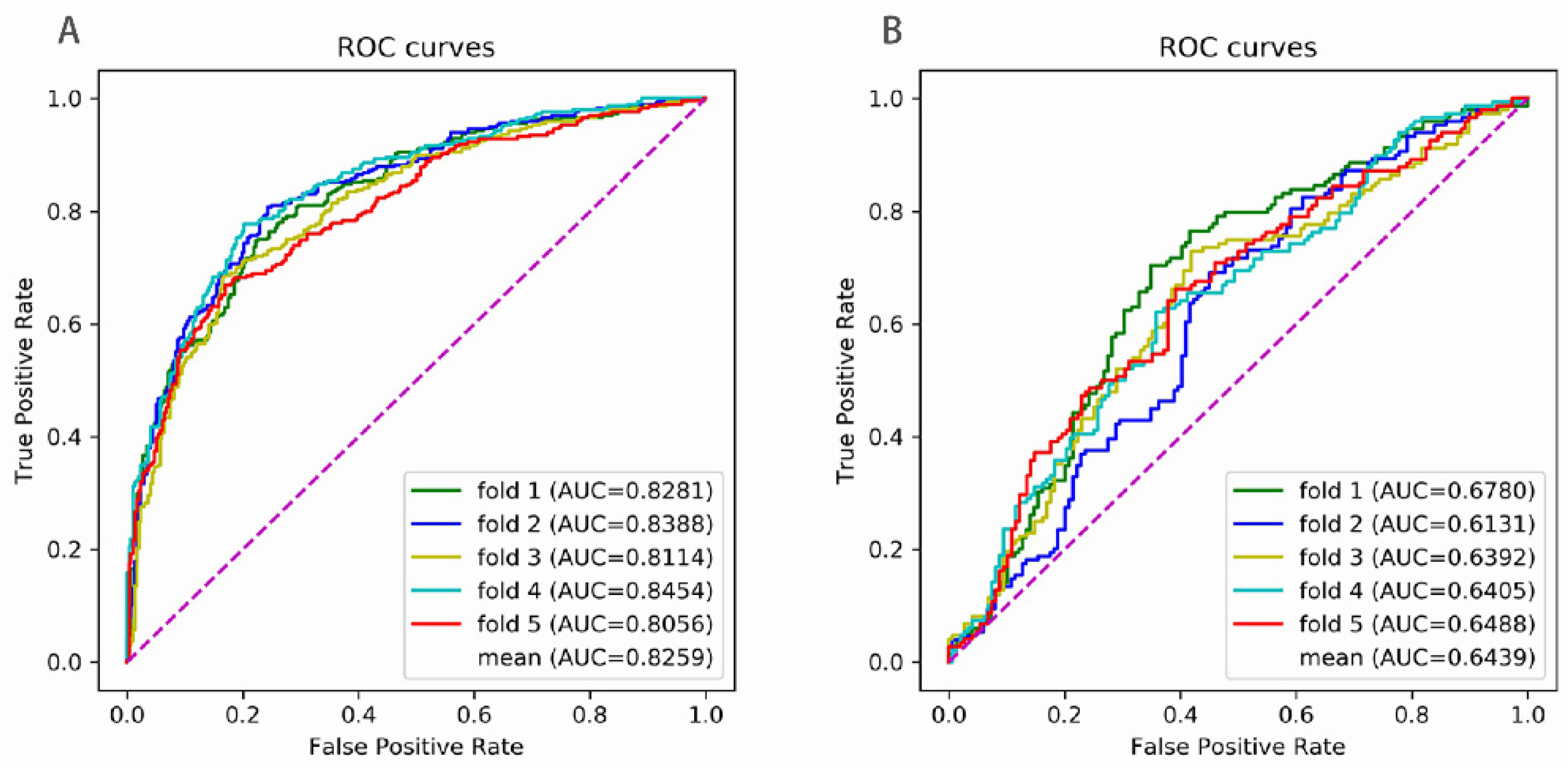
| fold 1 | 0.7374 | 0.7811 | 0.7593 | 0.5190 | 0.8281 |
| fold 2 | 0.8013 | 0.7576 | 0.7795 | 0.5595 | 0.8388 |
| fold 3 | 0.6801 | 0.8350 | 0.7576 | 0.5214 | 0.8114 |
| fold 4 | 0.7710 | 0.7980 | 0.7845 | 0.5692 | 0.8454 |
| fold 5 | 0.6622 | 0.8311 | 0.7466 | 0.5004 | 0.8056 |
| mean | 0.7304 | 0.8006 | 0.7655 | 0.5339 | 0.8259 |
| Second Stage | |||||
| fold 1 | 0.6846 | 0.6510 | 0.6678 | 0.3358 | 0.6780 |
| fold 2 | 0.6913 | 0.5369 | 0.6141 | 0.2310 | 0.6131 |
| fold 3 | 0.7297 | 0.5811 | 0.6554 | 0.3143 | 0.6392 |
| fold 4 | 0.6149 | 0.6419 | 0.6284 | 0.2569 | 0.6405 |
| fold 5 | 0.6622 | 0.6014 | 0.6318 | 0.2640 | 0.6488 |
| mean | 0.6765 | 0.6024 | 0.6395 | 0.2804 | 0.6439 |
| Method | Jackknife | 5-Fold | 10-Fold | Independent | Enhancer or Not | Strong or Weak |
|---|---|---|---|---|---|---|
| iEnhancer-2L [40] | √ | √ | √ | √ | ||
| iEnhancer-PsedeKNC [41] | √ | √ | √ | |||
| EnhancerPred [42] | √ | √ | √ | √ | ||
| EnhancerPred2.0 [43] | √ | √ | √ | |||
| Enhancer-Tri-N [44] | √ | √ | √ | |||
| iEnhaner-2L-Hybrid [45] | √ | √ | √ | |||
| iEnhancer-EL [46] | √ | √ | √ | √ | ||
| iEnhancer-5Step [47] | √ | √ | √ | √ | ||
| DeployEnhancer [48] | √ | √ | √ | √ | ||
| ES-ARCNN [49] | √ | √ | √ | |||
| iEnhancer-ECNN [50] | √ | √ | √ | |||
| EnhancerP-2L [51] | √ | √ | √ | √ | √ | |
| iEnhancer-CNN [52] | √ | √ | √ | √ | ||
| iEnhancer-XG [53] | √ | √ | √ | √ | ||
| Enhancer-DRRNN [54] | √ | √ | √ | |||
| Enhancer-BERT [55] | √ | √ | √ | |||
| iEnhancer-KL [56] | √ | √ | √ | |||
| iEnhancer-RF [57] | √ | √ | √ | √ | ||
| spEnhancer [58] | √ | √ | √ | |||
| iEnhancer-EBLSTM [59] | √ | √ | √ | |||
| iEnhancer-GAN [60] | √ | √ | √ | √ | ||
| piEnPred [61] | √ | √ | √ | √ | ||
| iEnhancer-RD [62] | √ | √ | √ | √ | ||
| iEnhancer-MFGBDT [63] | √ | √ | √ | √ |
| SN | SP | ACC | MCC | AUC | |
|---|---|---|---|---|---|
| Frist Stage | |||||
| iEnhancer-PsedeKNC [41] | 0.7731 | 0.7630 | 0.7678 | 0.5400 | 0.8500 |
| iEnhancer-5Step [47] | 0.8110 | 0.8350 | 0.8230 | 0.6500 | - |
| DeployEnhancer [48] | 0.7325 | 0.7642 | 0.7483 | 0.4980 | 0.7694 |
| EnhancerP-2L [51] | 0.9077 | 0.9259 | 0.9168 | 0.8340 | 0.9400 |
| iEnhancer-CNN [52] | 0.7588 | 0.8888 | 0.8063 | 0.6929 | 0.8957 |
| Enhancer-BERT [55] | 0.7950 | 0.7300 | 0.7620 | 0.5250 | - |
| iEnhancer-KL [56] | 0.8322 | 0.8524 | 0.8423 | 0.6800 | - |
| iEnhancer-RF [57] | 0.7364 | 0.7871 | 0.7618 | 0.5264 | 0.8400 |
| piEnPred [61] | 0.9228 | 0.8047 | 0.8788 | 0.7660 | 0.9603 |
| iEnhancer-RD [62] | 0.8100 | 0.7650 | 0.7880 | 0.5760 | 0.8440 |
| Enhancer-LSTMAtt | 0.7304 | 0.8006 | 0.7655 | 0.5339 | 0.8259 |
| Second Stage | |||||
| iEnhancer-PsedeKNC [41] | 0.6262 | 0.6441 | 0.6341 | 0.2700 | 0.6900 |
| iEnhancer-5Step [47] | 0.7530 | 0.6080 | 0.6810 | 0.3700 | - |
| DeployEnhancer [48] | 0.7965 | 0.3828 | 0.5896 | 0.1970 | 0.6068 |
| EnhancerP-2L [51] | 0.6221 | 0.6182 | 0.6193 | 0.2400 | 0.9000 |
| iEnhancer-CNN [52] | 0.7364 | 0.7680 | 0.7643 | 0.4505 | 0.8109 |
| iEnhancer-KL [56] | 0.9340 | 0.9287 | 0.9313 | 0.8600 | - |
| iEnhancer-RF [57] | 0.6846 | 0.5661 | 0.6253 | 0.2529 | 0.6700 |
| piEnPred [61] | 0.6554 | 0.7094 | 68.24 | 0.3654 | 0.7568 |
| iEnhancer-RD [62] | 0.8400 | 0.5700 | 0.7050 | 0.4260 | 0.7920 |
| Enhancer-LSTMAtt | 0.6765 | 0.6024 | 0.6395 | 0.2804 | 0.6439 |
| SN | SP | ACC | MCC | AUC | |
|---|---|---|---|---|---|
| Frist Stage | |||||
| EnhancerP-2L [51] | 0.8653 | 0.9690 | 0.9172 | 0.8398 | 0.9700 |
| iEnhancer-XG [53] | 0.7570 | 0.8650 | 0.8110 | 0.6265 | - |
| iEnhancer-GAN [60] | 0.9510 | 0.9510 | 0.9510 | 0.9020 | - |
| iEnhancer-MFGBDT [63] | 0.7754 | 0.7978 | 0.7867 | 0.5735 | - |
| Enhancer-LSTMAtt | 0.7414 | 0.7873 | 0.7658 | 0.5298 | 0.8256 |
| Second Stage | |||||
| ES-ARCNN [49] | 0.7278 | 59.57 | 66.17 | 0.3263 | 0.6604 |
| EnhancerP-2L [51] | 0.8049 | 0.9397 | 0.8723 | 0.7519 | 0.9300 |
| iEnhancer-XG [53] | 0.7494 | 0.5855 | 0.6674 | 0.3395 | - |
| iEnhancer-GAN [60] | 0.8730 | 0.8710 | 0.8720 | 0.7440 | - |
| iEnhancer-MFGBDT [63] | 0.7056 | 0.6163 | 0.6604 | 0.3232 | - |
| Enhancer-LSTMAtt | 0.6463 | 0.6380 | 0.6429 | 0.2851 | 0.6550 |
| SN | SP | ACC | MCC | AUC | |
|---|---|---|---|---|---|
| Frist Stage | |||||
| iEnhancer-2L [40] | 0.7100 | 0.7500 | 0.7300 | 0.4604 | 0.8062 |
| EnhancerPred [42] | 0.7350 | 0.7450 | 0.7400 | 0.4800 | 0.8013 |
| iEnhancer-EL [46] | 0.7100 | 0.7850 | 0.7475 | 0.4964 | 0.8173 |
| iEnhancer-5Step [47] | 0.8200 | 0.7600 | 0.7900 | 0.5800 | - |
| DeployEnhancer [48] | 0.7550 | 0.7600 | 0.7550 | 0.5100 | 0.7704 |
| iEnhancer-ECNN [50] | 0.7520 | 0.7850 | 0.7690 | 0.5370 | 0.8320 |
| EnhancerP-2L [51] | 0.7810 | 0.8105 | 0.7950 | 0.5907 | - |
| iEnhancer-CNN [52] | 0.7825 | 0.7900 | 0.7750 | 0.5850 | - |
| iEnhancer-XG [53] | 0.7400 | 0.7750 | 0.7575 | 0.5150 | - |
| Enhancer-DRRNN [54] | 0.7330 | 0.8010 | 0.7670 | 0.5350 | 0.8370 |
| Enhancer-BERT [55] | 0.8000 | 0.7120 | 0.7560 | 0.5140 | - |
| iEnhancer-RF [57] | 0.7850 | 0.8100 | 0.7975 | 0.5952 | 0.8600 |
| spEnhancer [58] | 0.8300 | 0.7150 | 0.7725 | 0.5793 | 0.8235 |
| iEnhancer-EBLSTM [59] | 0.7550 | 0.7950 | 0.7720 | 0.5340 | 0.8350 |
| iEnhancer-GAN [60] | 0.8110 | 0.7580 | 0.7840 | 0.5670 | - |
| piEnPred [61] | 0.8250 | 0.7840 | 0.8040 | 0.6099 | - |
| iEnhancer-RD [62] | 0.8100 | 0.7650 | 0.7880 | 0.5760 | 0.8440 |
| iEnhancer-MFGBDT [63] | 0.7679 | 0.7955 | 0.7750 | 0.5607 | - |
| Enhancer-LSTMAtt | 0.7950 | 0.8150 | 0.8050 | 0.6101 | 0.8588 |
| Second Stage | |||||
| iEnhancer-2L [40] | 0.4700 | 0.7400 | 0.6050 | 0.2181 | 0.6678 |
| EnhancerPred [42] | 0.4500 | 0.6500 | 0.5500 | 0.1020 | 0.5790 |
| iEnhancer-EL [46] | 0.5400 | 0.6800 | 0.6100 | 0.2222 | 0.6801 |
| iEnhancer-5Step [47] | 0.7400 | 0.5300 | 0.6350 | 0.2800 | - |
| DeployEnhancer [48] | 0.8315 | 0.4561 | 0.6849 | 0.3120 | 0.6714 |
| ES-ARCNN [49] | 0.8600 | 0.4500 | 0.6560 | 0.3399 | - |
| iEnhancer-ECNN [50] | 0.7910 | 0.5640 | 0.6780 | 0.3680 | 0.7480 |
| EnhancerP-2L [51] | 0.6829 | 0.7922 | 0.7250 | 0.4624 | - |
| iEnhancer-CNN [52] | 0.6525 | 0.7610 | 0.7500 | 0.3232 | - |
| iEnhancer-XG [53] | 0.7000 | 0.5700 | 0.6350 | 0.2720 | - |
| Enhancer-DRRNN [54] | 0.8580 | 0.8400 | 0.8490 | 0.6990 | - |
| iEnhancer-RF [57] | 0.9300 | 0.7700 | 0.8500 | 0.7091 | 0.9700 |
| spEnhancer [58] | 0.9100 | 0.3300 | 0.6200 | 0.3703 | 0.6253 |
| iEnhancer-EBLSTM [59] | 0.8120 | 0.5360 | 0.6580 | 0.3240 | 0.6880 |
| iEnhancer-GAN [60] | 0.9610 | 0.5370 | 0.7490 | 0.5050 | - |
| piEnPred [61] | 0.7000 | 0.7500 | 0.7250 | 0.4506 | - |
| iEnhancer-RD [62] | 0.8400 | 0.5700 | 0.7050 | 0.4260 | 0.7920 |
| iEnhancer-MFGBDT [63] | 0.7255 | 0.6681 | 0.6850 | 0.3862 | - |
| Enhancer-LSTMAtt | 0.9900 | 0.8000 | 0.8950 | 0.8047 | 0.9637 |
Publisher’s Note: MDPI stays neutral with regard to jurisdictional claims in published maps and institutional affiliations. |
© 2022 by the authors. Licensee MDPI, Basel, Switzerland. This article is an open access article distributed under the terms and conditions of the Creative Commons Attribution (CC BY) license (https://creativecommons.org/licenses/by/4.0/).
Share and Cite
Huang, G.; Luo, W.; Zhang, G.; Zheng, P.; Yao, Y.; Lyu, J.; Liu, Y.; Wei, D.-Q. Enhancer-LSTMAtt: A Bi-LSTM and Attention-Based Deep Learning Method for Enhancer Recognition. Biomolecules 2022, 12, 995. https://doi.org/10.3390/biom12070995
Huang G, Luo W, Zhang G, Zheng P, Yao Y, Lyu J, Liu Y, Wei D-Q. Enhancer-LSTMAtt: A Bi-LSTM and Attention-Based Deep Learning Method for Enhancer Recognition. Biomolecules. 2022; 12(7):995. https://doi.org/10.3390/biom12070995
Chicago/Turabian StyleHuang, Guohua, Wei Luo, Guiyang Zhang, Peijie Zheng, Yuhua Yao, Jianyi Lyu, Yuewu Liu, and Dong-Qing Wei. 2022. "Enhancer-LSTMAtt: A Bi-LSTM and Attention-Based Deep Learning Method for Enhancer Recognition" Biomolecules 12, no. 7: 995. https://doi.org/10.3390/biom12070995
APA StyleHuang, G., Luo, W., Zhang, G., Zheng, P., Yao, Y., Lyu, J., Liu, Y., & Wei, D.-Q. (2022). Enhancer-LSTMAtt: A Bi-LSTM and Attention-Based Deep Learning Method for Enhancer Recognition. Biomolecules, 12(7), 995. https://doi.org/10.3390/biom12070995