Article

Double-Layer RRT* Objective Bias Anytime Motion Planning Algorithm

1
Department of Electronics and Communication Engineering, College of Engineering, A’Sharqiyah University, Ibra 400, Oman
2
Department of Electrical Engineering, Faculty of Engineering, Aswan University, Aswan 81542, Egypt
3
College of Electronic Science and Technology, Xiamen University, Xiamen 361005, China
4
School of Electronic and Computer Engineering, Peking University, Shenzhen 518005, China
5
Department of Information and Communication, School of Informatics, Xiamen University, Xiamen 316005, China
*
Author to whom correspondence should be addressed.
Robotics 2024, 13(3), 41; https://doi.org/10.3390/robotics13030041
Submission received: 13 January 2024 / Revised: 11 February 2024 / Accepted: 13 February 2024 / Published: 1 March 2024
(This article belongs to the Section Sensors and Control in Robotics)

Abstract

:
This paper proposes a double-layer structure RRT* algorithm based on objective bias called DOB-RRT*. The algorithm adopts an initial path with an online optimization structure for motion planning. The first layer of RRT* introduces a feedback-based objective bias strategy with segment forward pruning processing to quickly obtain a smooth initial path. The second layer of RRT* uses the heuristics of the initial tree structure to optimize the path by using reverse maintenance strategies. Compared with conventional RRT and RRT* algorithms, the proposed algorithm can obtain the initial path with high quality, and it can quickly converge to the progressive optimal path during the optimization process. The performance of the proposed algorithm is effectively evaluated and tested in real experiments on an actual wheeled robotic vehicle running ROS Kinetic in a real environment.

1. Introduction

Planning is often applied to determine how to move along; the solution should be provided in a way that complies with the mechanical limitations of autonomous systems, such as robotics [1,2], graphic animation [3], manufacturing [4], and minimally invasive surgical procedures [5]. In the state space, the problem of robot motion planning [6,7,8] involves starting in some initial state and trying to arrive at a specified goal instead of goal states to minimize resource consumption, such as energy or time.
Rapidly exploring random tree (RRT) [9] is one of the most popular approaches applied to handle nonholonomic problems of path planning in a high-dimensional configuration space. RRT’s unique advantage is that it does not require any connections between configurations in pairs of states; hence, it can directly be applied to nonholonomic and Kino dynamic planning [10,11,12,13,14,15,16,17]. In robot navigation problems, RRT addresses the path planning problem by creating a random extended tree to find a suitable path, but, unfortunately, the RRT-suggested path can be a non-optimal one. To handle this issue, a modified RRT algorithm called RRT* has been proposed by Karaman and Frazzoli [18]. The RRT* algorithm tries to obtain the shortest path, whether by distance or other metrics. The modified RRT algorithm RRT* improves the path quality by introducing the major features of tree rewiring and a best neighbor search. However, it obtains asymptotic optimality at the expense of the execution time and convergence rate.
The RRT*-variant-based scheme has been proposed as an anytime scheme [19,20]. The main feature of the anytime scheme is that the planned time is unknown in advance, and it can be terminated at any time. When time permits, any solution should be obtained as soon as possible, and then the chosen solution should be updated to be more conventional. The RRT*-variant anytime algorithm’s [19,20] criteria are to firstly and quickly obtain some motion plans; these plans are not necessarily optimal but feasible. Then, RRT* is used to improve the path quality online over time. The lower bound tree-RRT (LBT-RRT) [21] allows continuous interpolation between RRT, RRT*, and RRG and achieves high-quality anytime motion planning by maintaining two roadmaps at the same time. The R R R X proposed in [22] first obtains the initial plan and refines it to be the best solution through continuous repair. In [23], a doubletree RRT* (DT-RRT*) has been proposed based on a dual-tree structure to separate the expansion process from the optimization process. DT-RRT* initiates the path through the expansion process and the shortcut principle is used for optimization. However, unfortunately, the current anytime algorithms cannot support the new generation of unmanned driving systems due to the long latency time, in addition to inaccurate path selection metrics as the smoothing path quality is not considered in these schemes.
To cope with the new generation of unmanned driving systems’ requirements, this paper proposes a real-time anytime planning algorithm suitable for unmanned driving systems. To address the drawbacks of the current anytime motion planning schemes, the proposed anytime planning algorithm adopts the initial path and online-optimized double-layer structure for motion planning, considering the latency time in addition to the selected path smoothing level. In the proposed scheme, the first layer of the RRT* scheme uses a feedback-based biased sampling strategy to obtain the initial path and uses segment forward pruning processing to evaluate the smoothing level of the selected initial path. The second layer in the RRT* scheme performs the online optimization of the selected initial path, which adopts the reverse maintenance spanning-tree scheme. In summary, the main contributions of this paper are as follows.
(1)
This paper proposes a double-layer RRT* tree structure. In the first layer, initial path information is provided. In the second layer, an iterative optimization process is used to update the selected path and improve the path selection accuracy.
(2)
A new feedback-based objective bias strategy is used to obtain the initial path, and the initial path is smoothed by removing redundant processing through segmentation forward pruning.
(3)
The second layer of the RRT* scheme optimizes the selected path using the heuristic information provided by the spanning tree structure of the initial path.
Compared to the conventional RRT and RRT*, the proposed algorithm can allow the path to gradually approach the optimal solution while ensuring the running speed.
The rest of the paper is as follows. In Section 2, the problem of motion planning is stated. In Section 3, the initial path generation algorithm is described in detail. In Section 4, the optimization algorithm is described in detail. In Section 5 and Section 6, the performance of the proposed scheme is assessed in an experiment in a real environment. Finally, the paper is concluded in Section 7.

2. Motion Planning Problem Statements

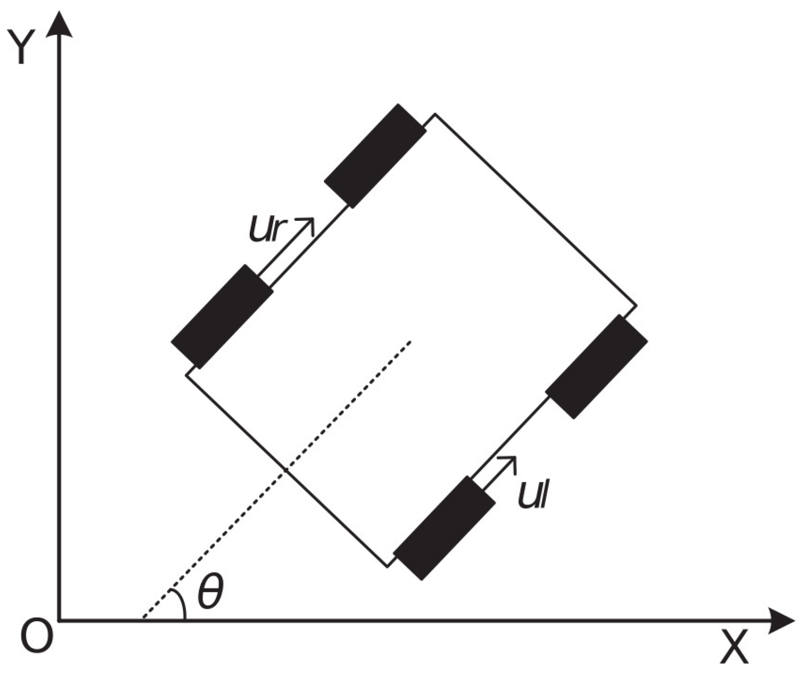
2.1. Robot Model and Control Input

The two-wheel differential robot model discussed in this paper is shown in Figure 1. The dynamic models of the two-wheel model are described as follows.
x ˙ = x ˙ y ˙ θ ˙ = cos θ 0 sin θ 0 0 1 u r u l ,
where x ˙ = x ˙ ,   x ˙ , θ is the state vector, which is used as the control input of the robot. This state vector is determined by the Cartesian coordinate system x , y , the operation θ , and the dynamic constraints u r and u l . In addition, two-wheeled differential robots generally have no backward motion and can support rotation in place.

2.2. Problem Statement

The motion planning problem is used to calculate a continuous path from the initial configuration q s t a r t to the goal state q g o a l , avoiding collision with existing obstacles. Assuming that the environment and the geometry of the robot are described in an n -dimensional state space, the motion plan can be expressed as a path in the state space. Let q R n   n -dimensional configuration space C [24] and C o b s is the obstacle region. Therefore, C f r e e = C / C o b s can be used to represent the free region of the configuration space. In the RRT algorithm, the spanning tree is represented as T = ( V ,   E ) , where V is the set of vertices of the spanning tree in the configuration space and E is the set of edges between vertices. RRT expands the spanning tree T by searching for random samples in the configuration space. The goal of the exercise plan is to return the trajectory τ t   :   0 , s     C f r e e , where τ 0 = q s t a r t ,   τ s = q g o a l , corresponding to the control input causing the robot to move from q s t a r t to q g o a l .

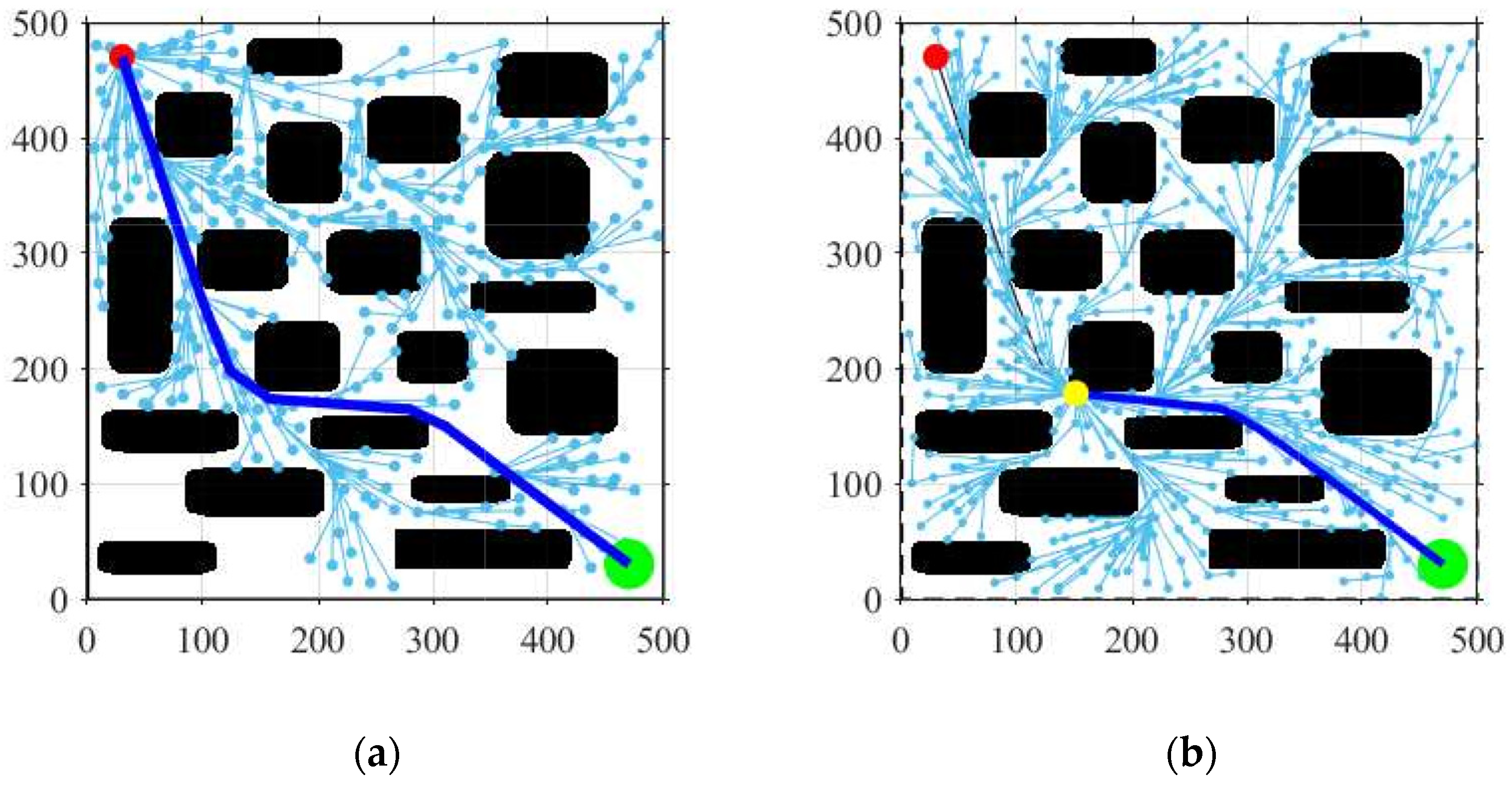
3. Initial Path Generation Algorithm

In this section, we introduce and discuss the proposed initial path acquisition algorithm using an objective bias strategy and segmented forward pruning.

3.1. Initial Path Generation

Before navigation, the initial path is generated by the first layer in RRT*. Algorithm 1 shows the overall flow of the proposed initial path generation algorithm. The input parameters of the algorithm include the binary map of the environment m a p , the initial point q s t a r t , and the goal point q g o a l . The following terms are used to describe the algorithm.
O b j B i a s S a m p l e ( ) : returns the random node q r a n d x , y in the free configuration.
F i n d Q N e a r e s t ( q ,   V ) : finds the nearest node to q r a n d x , y from the current spanning tree by Euclidean distance.
F i n d Q N e a r S e t s ( q ,   V ) : returns the set of all nodes within r range near q r a n d from the current spanning tree.
S t e e r q 1 , q 2 : a partial path from q 1 to q 2 .
C o l l i s i o n D e t e c t i o n   q 1 , q 2 : connects q 1 and q 2 and judges whether the connection has an intersection with the obstacle.
C h o o s e P a r e n t   q 1 , q 2 : finds the nearest neighbors within a defined radius around the node q 1 as a candidate to replace the parent node of q 2 .
R e w i r e   q 1 , q 2 : after reselecting the parent node for q 1 , performs rewiring to ensure that the cost of the connection between the random tree nodes is as small as possible.
C o s t ( q ) : returns the cost value of the path from the root nodes of the spanning tree to q .
D i s t a n c e C o s t q 1 , q 2 : returns the cost value of the path between q 1 and q 2 .
P a t h P r u n i n g ( V ,   E ) : uses the segment forward pruning strategy to optimize the path.
Algorithm 1.  T = Build Initial Path m a p , q s t a r t ,   q g o a l .
1: V q s t a r t ; E = ; T = V , E ;
2: for i from 0 to K do
3:  q r a n d   O b j B i a s S a m p l e ( ) ;
4:  q n e a r   F i n d Q N e a r e s t V , q r a n d ;
5:  q n e w   S t e e r q n e a r , q r a n d ;
6: if C o l l i s i o n D e t e c t i o n   q n e a r , q n e w then
7:   q n e w = q t e m p ;
8: else
9:   C o n t i n u e ;
10:  end if
11:   Q n e a r F i n d Q N e a r S e t s q n e w , V , r ;
12:  for q n e a r Q n e a r do
13:   T C h o o s e P a r e n t q n e a r , q n e a r ;
14:   T R e w i r e q n e a r , q n e a r ;
15:  end for
16:   C c u r C o s t T ;
17:  if D i s t a n c e q n e w , q g o a l d m i n then
18:  return T = V , E ;
19:  end if
20: end for
21: T P a t h P r u n i n g V , E ;
The difference between the proposed initial path generation algorithm and the conventional RRT* algorithm is mainly in the method of selecting sampling points and adding post-prune processing. O b j B i a s S a m p l e ( ) in the third line of Algorithm 1 is the objective-biased sampling strategy. After q n e w is added to the tree at the minimum cost, the rewire optimization process is performed. First, obtain the set Q n e a r , which is the node within the distance r around q n e w . Then, calculate the cost for each q n e a r in the set Q n e a r and select the node with the smallest cost as the parent node of q n e w . Finally, check whether q n e w can be the parent node of each q n e a r ; if yes, connect the new line. As the tree expands to q g o a l , the algorithm returns the path node. Because of the existence of multiple redundant nodes on this path, a segmented forward pruning strategy is proposed for optimization, as shown in the 14th line of Algorithm 1.

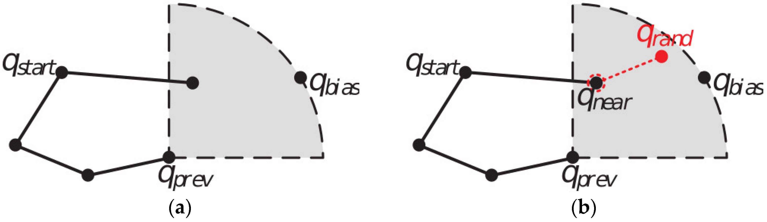
3.2. Objective-Biased Sampling Strategy

Figure 2 shows the node expansion strategy of the conventional RRT*; the node q s t a r t is the initial position, and the node q n e a r is a node that has been added to the spanning tree. As shown in Figure 2a, the node q r a n d is a random sampling point in C f r e e . The new node q n e w in Figure 2b is generated by RRT* to the random sampling point q r a n d with an appropriate extension length. Due to the global randomness of the points taken by the conventional RRT*, it often leads to an excessive search on the map.
The feedback-based biased sampling strategy proposed in this paper uses the probability P to refer to the node q p r e v that is added to RRT* as a reference and reduces the sampling area of q r a n d by q p r e v for a relative position and the goal state, enhancing the inspiration of the goal state. The relationship between q p r e v and the goal state q b i a s is used as a reference for the next selected point, as shown in Figure 3. At this time, q b i a s is located in the upper right corner of q p r e v , choosing a quarter-circle area with q p r e v as the center. The distance between q p r e v and q b i a s is considered as the radius of the sampling point selection area. By this method, under the premise of ensuring random sampling, there is a probability P of obtaining biased sampling points, avoiding unnecessary or excessive searches and speeding up the acquisition of the initial path.

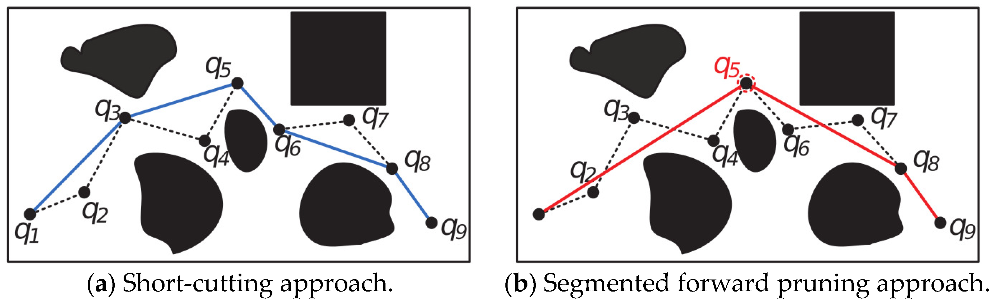
3.3. Segmented Forward Pruning

Under normal circumstances, the paths obtained through the RRT* and RRT*-variant algorithms are generally more complicated and tortuous paths, including more unnecessary and redundant nodes. To ensure the high-speed navigation of the robot, the generated path must remove as many nodes as necessary under the premise of ensuring no collision. The algorithm uses pruning to obtain a shorter and less tortuous initial path. The short-cutting approach [25] has been widely used to eliminate the pruning operation of redundant nodes. In Figure 4, let q 1 be the starting point, q 9 the endpoint, and the dotted line segment as the initial path. The short-cutting approach starts from q 1 to connect other nodes in sequence, i.e., connect q 1 to q 3 first and judge whether the connection is legal. If there is no intersection with the obstacle, delete the other nodes between q 1 and q 3 . Until the line collides, i.e., q 1 and q 4 intersect with the obstacle, repeat the above operation with q 3 as a new starting point until finally reaching the goal state q 9 . The resulting path is shown in the blue line in Figure 4a. An obvious defect of this pruning method is that the current connection stops prematurely. For example, if q 1 and q 4 cannot be connected, the connection to the next starting point q 3 is entered. However, we can see that q 1 and q 5 can be connected. Such a result will lead to poor pruning. We modify the short-cutting approach and propose a segmented forward pruning approach. As shown in Figure 4b, the node at the midpoint is selected to divide the path into two segments, i.e., one segment from the start point to the midpoint and one segment from the midpoint to the endpoint. The sequential connection is changed to the reversed connection, i.e., we first determine whether q 1 and q 6 can be connected. If the connection is illegal, the search will continue to determine the connection between q 1 and q 5 , and so on. This method can effectively avoid the situation in which the redundancy removal of the traditional pruning method is not thorough enough.

4. Optimization Algorithm

In this section, we introduce the proposed path optimization algorithm using a reverse maintenance strategy.

4.1. Optimization Algorithm

After submitting the initial path, the robot obtains an initial motion plan. Since only one path is solved, the path cannot guarantee the optimal solution. Therefore, we make the path asymptotically optimal through the optimization algorithm, which uses a reverse maintenance strategy. The optimization process will continue until the robot reaches the goal state. Algorithm 2 shows the overall flow of the optimization algorithm. The algorithm initializes by q g o a l as the root node q r o o t ; then, in the fourth line, U p d a t e L o c a t i o n ( ) updates the robot position; in the fifth line, H e u r i s t i c S a m p l e ( ) uses the heuristic information provided by the initial path for sampling; and the eighteenth line calculates the cost of the current path.
Algorithm 2.  T = Optimization m a p , T I n i t i a l ,   q g o a l .
1: T T I n i t i a l ; q r o o t q g o a l ;
2: C m i n C o s t T ;
3: while  N o t r e a c h G o a l  do
4:    U p d a t e L o c a t i o n ( ) ;
5:    q r a n d   H e u r i s t i c S a m p l e ( ) ;
6:    q n e a r   F i n d Q N e a r e s t V , q r a n d ;
7:    q t e m p = S t e e r q n e a r , q r a n d ;
8:   if  C o l l i s i o n D e t e c t i o n q n e a r , q n e w  then
9:   q n e w = q t e m p ;
10:  else
11:    C o n t i n u e ;
12:  end if
13:   Q n e a r F i n d Q N e a r S e t s q n e w , V , r ;
14:  for  q n e a r Q n e a r  do
15:    T C h o o s e P a r e n t q n e w , q n e a r ;
16:    T R e w i r e q n e w , q n e a r ;
17:  end for
18:   C c u r C o s t T ;
19:  if C c u r < C m i n  then
20:    C m i n C c u r ;
21:    T r a j e c t o r y T r a c t i o n B S p l i n e T ;
22:  end if
23: end while

4.2. Reverse Maintenance Strategy

The second layer of the RRT* scheme is a reverse maintenance strategy, i.e., using q g o a l as a root node of DOB-RRT* to expand, which makes it easy for the planner to calculate C o s t T o G o ( ) and obtain the residual path cost. In the proposed DOB-RRT* scheme, the heuristic information provided by the initial path will be used with a certain probability P based on the initial path node and reference node q r e f . The sampling points are obtained through the relative positions of q r e f and q s t a r t , and the sampling area selection will be consistent with the selection method explained in Section 3.
In the proposed DOB-RRT* scheme, the cost function is modified to consider the E u c l i d e a n distance and trajectory angle to improve the rationality of the cost function. In practical applications, the path generated by the algorithm needs to be as smooth as possible, which can reduce the speed change of the mobile robot and increase the execution speed. Therefore, the optimal path not only needs to consider the path length but also the smoothness of the path. As depicted in Figure 5, in the selection process of the parent node and after a new node q n e w is obtained, the candidate parent nodes are q 1 and q 2 , and the extension paths from the root node q r o o t to q n e w are e 1 and e 2 , respectively. If we consider the E u c l i d e a n distance and trajectory angle to select q 2 as a parent node of q n e w , this means that although the path length of e 1 is shorter than that of e 2 , the path of e 2 is smoother than that of e 1 .
Hence, the path of e 2 will reduce the speed change of the robot in practical applications. Because the distance and angle are different types of data, they need to be normalized before comprehensive consideration. The cost function is defined as
C o s t q n e w , q i = λ d d q n e w , q i d m i n d m a x d m i n + λ θ θ q n e w , q i θ m i n θ m a x θ m i n ,
λ d + λ θ = 1       a n d   λ d , λ θ 0,1 ,
where d q n e w , q i is the E u c l i d e a n distance between the new node q n e w and node q i , and d m a x , d m i n represent the maximum and minimum distances between q n e w and nearby nodes, respectively. The angle value of the path between the new node q n e w and node q i is θ q n e w , q i , and the maximum and minimum distances of the angle value of the path between q n e w and nearby nodes are expressed as θ m a x and θ m i n , respectively. The weights of the distance and angle in the cost function are λ d and λ θ , respectively. The cost function can be adapted to different requirements by modifying the weights of the distance and angle. The substitute value of each node is a cumulative sum of the costs from the current node to the root node.

5. Simulation and Experimental Results

In this section, we conduct some numerical simulations to test the effectiveness of our proposed motion planning algorithm. The first simulation compares the initial path generation method with the RRT algorithm, and the other simulation verifies the feasibility of the DOB-RRT* algorithm. The simulation is performed in MATLAB 2020a, and the computer used is an i7-8700 CPU with 16G memory.

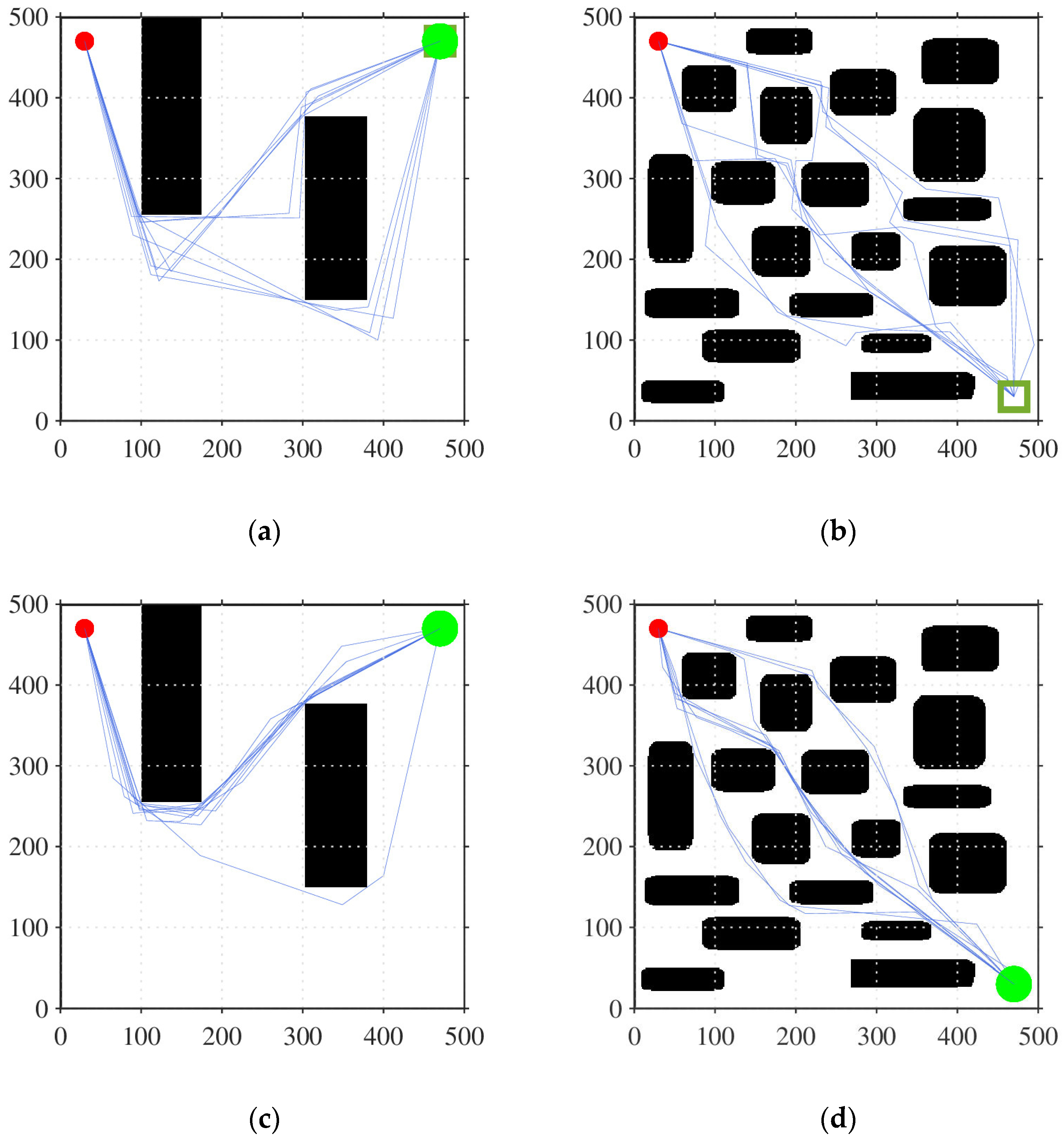
5.1. Initial Path Generation Simulation

First, we verify the effectiveness of the initial path generated by DOB-RRT* and select RRT and RRT* for comparison. We choose two maps for simulation. One is a map with dense obstacles and the other is a map with only two obstacles, and the size of both maps is 500 × 500 . In addition, the initial path generated by DOB-RRT* uses a segmented forward pruning strategy to optimize the path length. To achieve the contrast effect, we also perform the same pruning process on the paths generated by RRT and RRT*.
Figure 6 illustrates the paths generated by 10 simulations for each algorithm. Table 1 and Table 2 show the result statistics of 100 simulations for each algorithm, including the time required to generate the path and the quality of the selected path, which is represented by the length of the path. The simulation results show that RRT takes the smallest amount of time to generate a path, but RRT cannot guarantee the path quality. RRT* can guarantee the path quality better than RRT, but it takes a long time. Although DOB-RRT* requires slightly more time to generate a path than RRT, it is better than the conventional RRT scheme in terms of path quality. Compared with RRT*, the proposed DOB-RRT* is better than RRT* in terms of the time required to generate the path, while the path quality is similar to that of RRT*. In addition, DOB-RRT* has better stability in maps with dense obstacles. In summary, these results show that DOB-RRT* is intermediate between RRT and RRT* and it is feasible to obtain high-quality initial paths within an acceptable latency time.

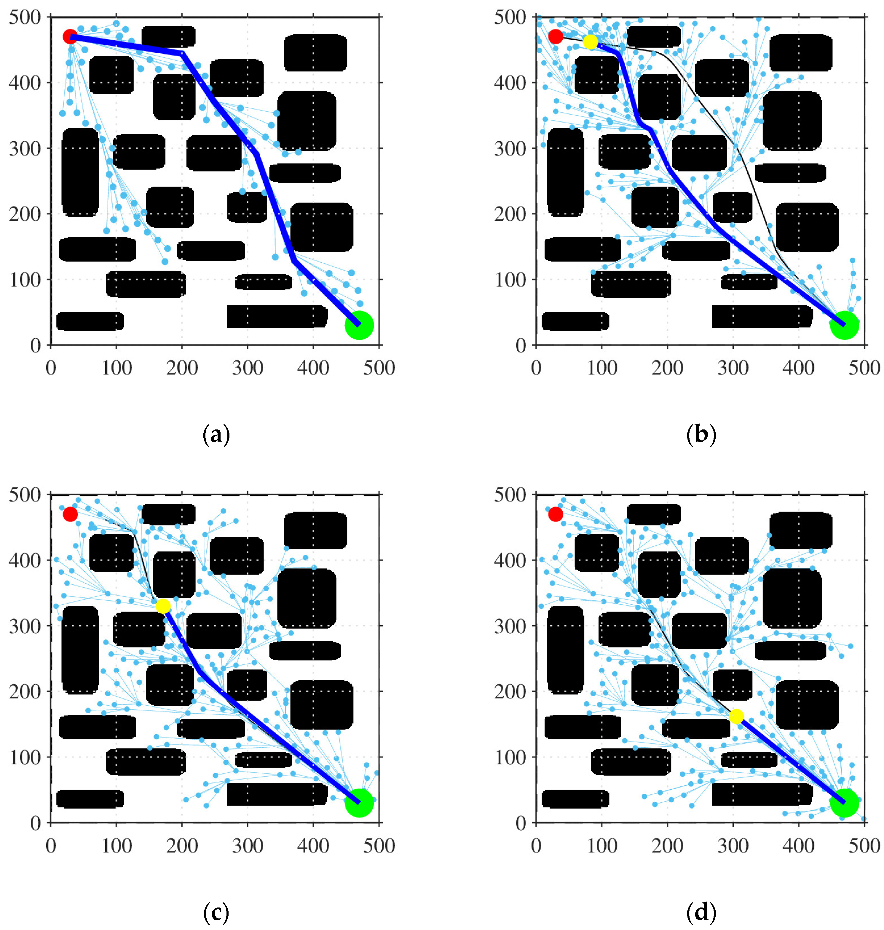
5.2. Optimization Simulation

We choose a map with dense obstacles as an environment for the online optimization simulation with a map size of 500 × 500 (pixels). Considering the simulated robot as a point, the maximum linear velocity of the robot is set to be 1   m / s , and the maximum acceleration is set to be 0.5   m / s 2 . The planner first needs to find a feasible path from the initial point shown by the red dot in the upper left corner of the environment to the goal area shown as a green area. From our simulation and verification of the effectiveness of the proposed DOB-RRT* in online optimization, we select RRT* for comparison.
The simulation result of the proposed DOB-RRT* in real-time optimization is shown in Figure 7. The yellow dot in Figure 7 represents the current position of the robot, and the blue line represents the currently executed plan. Figure 7a shows the initial path and state tree structure, allowing the robot to travel along a relatively expensive path. When the robot starts to execute the plan, the number of states optimized online obtains a lower-cost route; see Figure 7b. The process of online optimization will continue until the robot reaches the goal area. We compare the proposed DOB-RRT* scheme with the conventional RRT* in terms of the generated path; the simulation results of the online optimization based on RRT* are shown in Figure 8. The simulation results of each algorithm are listed in Table 3. T i represents the time required to calculate the initial path, and T o represents the average time required for online optimization.
From the simulation results, we can see that a shorter time is required by the proposed DOB-RRT* to obtain the initial path compared to the conventional RRT* scheme and it can converge to the asymptotically optimal path faster. As the RRT* online optimization calculation time is longer, the robot has already executed some of the costlier paths. DOB-RRT*’s online optimization solution can optimize the tree structure using the execution plan time and improve the path quality, including the path length and smoothness. The optimization of the proposed DOB-RRT* scheme allows it to find the path faster than the conventional RRT* scheme by 400   m s . This search time reduction in the proposed DOB-RRT* scheme proves that it can be effective in online optimization and is suitable for unmanned driving systems.

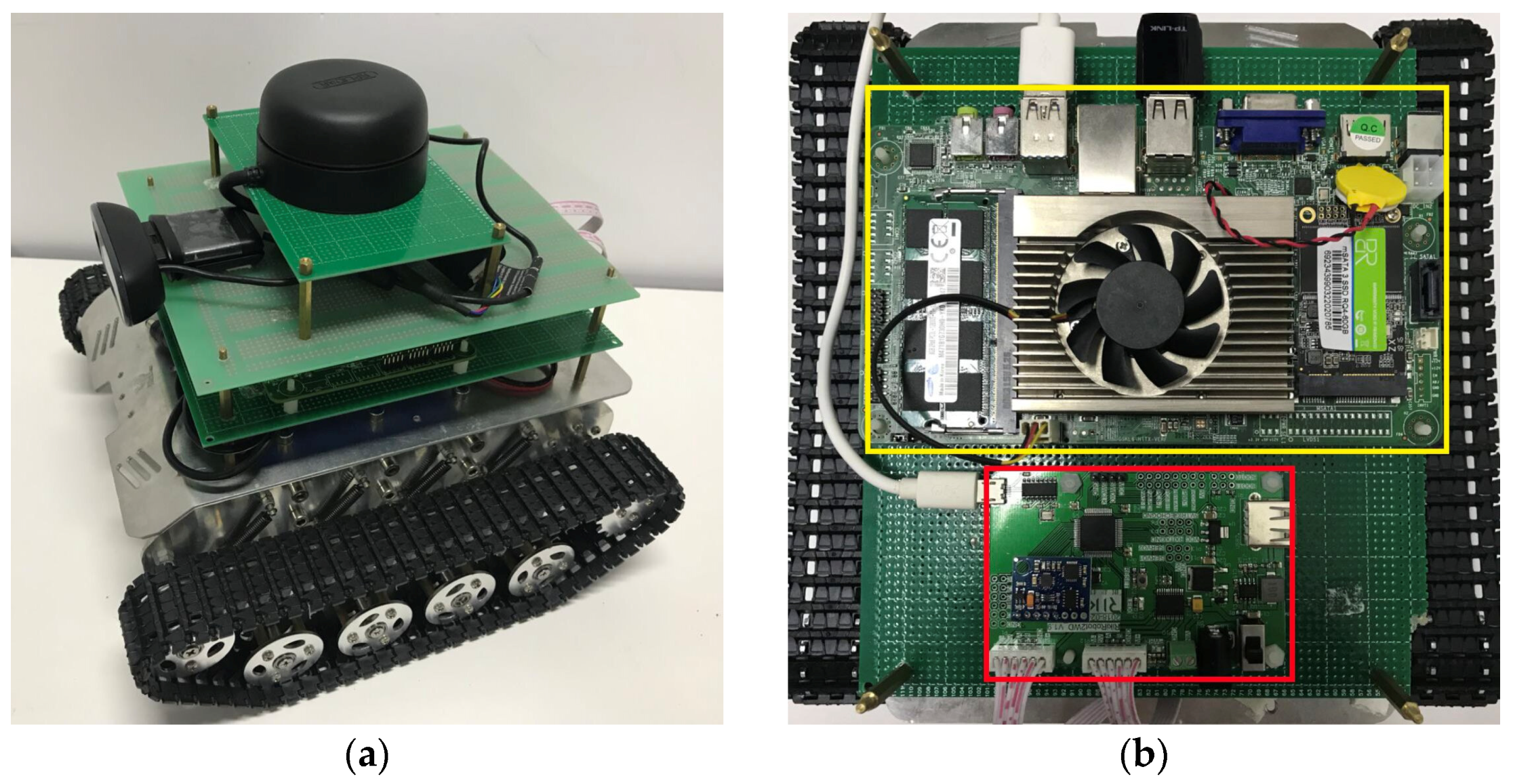
6. DOB-RRT* Evaluations in Real Environment

6.1. Experimental Environment Configuration

To prove the validity of the proposed path-tracking algorithm in a real environment, a real experiment is performed. The tracked robot used in this experiment is shown in Figure 9a. The vehicle size is 270   m m × 222   m m with a 229   m m wheelbase. An industrial computer with an i7-7500U processor (the yellow lined area in Figure 9b) and running the Kinetic robot operating system (ROS) is used in these experiments. The mapping package supported by the ROS is used to build the environment map. The adaptive Monte Carlo Positioning (AMCL) package is used for robot self-positioning and updates the real-time position. The STM32F103 (the red-lined area in Figure 9b) is used to communicate with the ROS software and control the robot motor. In this experiment, the maximum linear velocity of the robot is set to 0.5   m / s , with 0.2   m / s 2 maximum acceleration. When the robot is less than 5   c m from the goal state, we consider the robot to have reached the goal state.

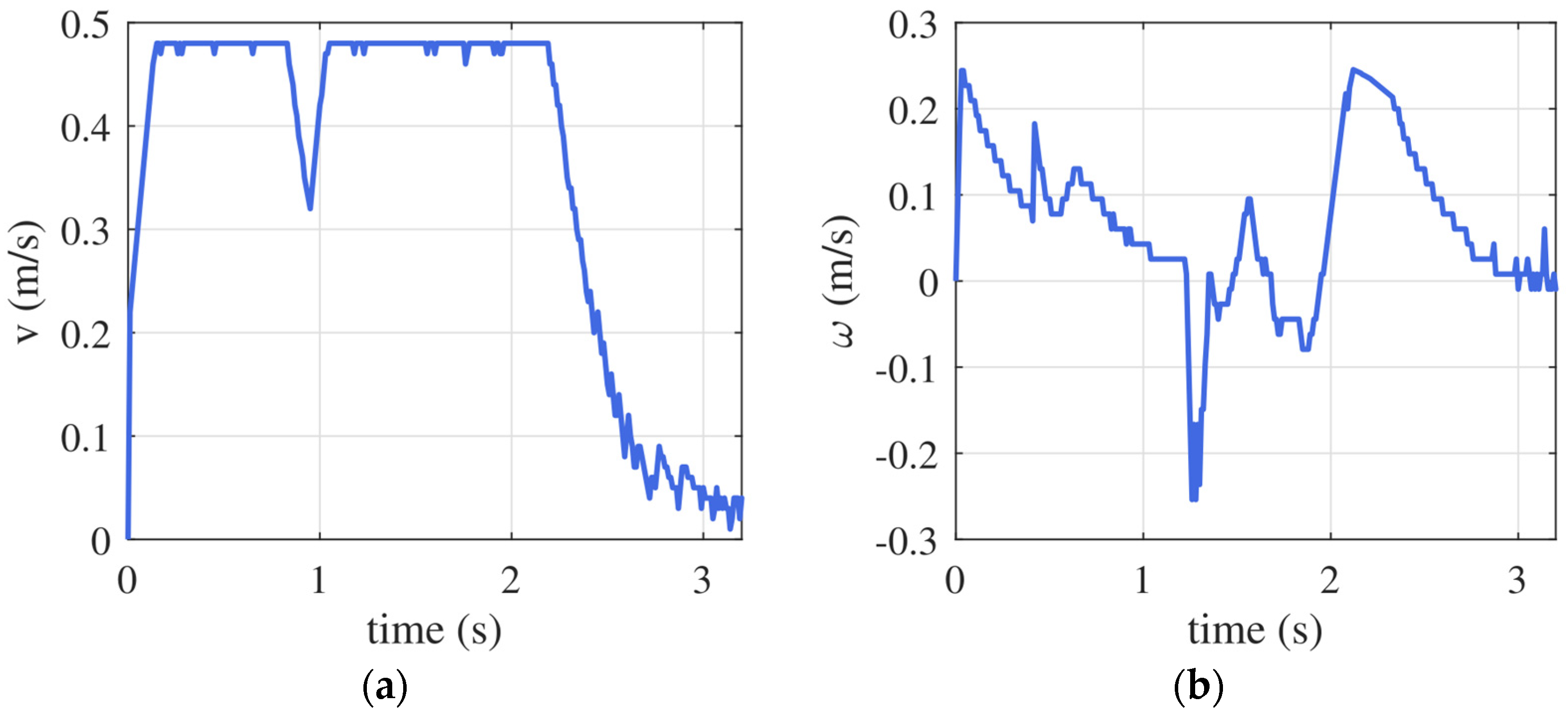
6.2. Mobile Robot Applications

To further verify the effectiveness of the algorithm in the actual environment, we conduct indoor experiments. The experiment is carried out using a crawler robot, as shown in Figure 9. We implement our motion planning algorithm in the ROS environment. Motion planning algorithms can also be transplanted to other robots running ROS. The experimental environment is shown in Figure 10. As illustrated in Figure 10a, in the beginning, and based on the surrounding environment, using a laser point, the robot can generate a laser point cloud map. This cloud map is stored as its recognized map. The initial path generated by the first layer of RRT* is shown in Figure 11a, and the optimized path obtained by the second layer of RRT* is shown in Figure 11b. The time required for the robot to complete the navigation is 3.26   s , and the values of the linear velocity and angular velocity during navigation are shown in Figure 12. The detailed data of the operation are shown in Table 4. Based on these detailed data collected from the real experiment, the robot can quickly find the initial path based on the proposed DOB-RRT* algorithm and use the online optimization plan to improve the path quality during the execution of the plan. From the experimental results, we can see the strong similarity between the data obtained from the real experiment and the data obtained from the simulation results.

7. Conclusions

This paper studies the problem of motion planning in an anytime motion scenario, focusing on the online solving and real-time optimization of motion planning problems. To achieve this goal, a double-layer RRT* algorithm is proposed. The proposed DOB-RRT* algorithm uses one tree to explore the initial path and another tree to optimize and update the selected path. The performance of the proposed DOB-RRT* algorithm is evaluated in a simulation and real experiments. The simulation results show that the proposed DOB-RRT* algorithm can reduce the calculation cost of the planned path. The proposed DOB-RRT* is superior to other reference algorithms in terms of its stability, path length, and smoothness. Through practical applications, we verify the effectiveness of the DOB-RRT* algorithm in real environments. In future research, the construction of a motion planning algorithm for multi-robot collaborative work will be conducted.

Author Contributions

Conceptualization, H.E. and G.Z.; methodology, H.E., G.Z. and Z.A.H.Q.; software, H.E. and G.Z.; validation, J.Q., H.S. and H.E.; formal analysis, Z.A.H.Q. and H.S.; investigation, Z.A.H.Q. and J.Q.; resources, H.E., Z.A.H.Q. and G.Z.; data curation, H.E. and G.Z.; writing—original draft preparation, H.E. and G.Z.; writing—review and editing, Z.A.H.Q., J.Q. and H.S.; visualization, H.E., J.Q. and H.S.; supervision, J.Q. and H.S.; project administration, J.Q. and H.S.; funding acquisition, J.Q. and H.S. All authors have read and agreed to the published version of the manuscript.

Funding

This research received no external funding.

Data Availability Statement

The authors declare that the data used to support the findings of this study will be available from the corresponding author upon request.

Conflicts of Interest

The authors declare no conflicts of interest.

References

  1. Latombe, J.-C. Motion planning: A journey of robots, molecules, digital actors, and other artifacts. Int. J. Robot. Res. 1999, 18, 1119–1128. [Google Scholar] [CrossRef]
  2. Gao, H.; Hou, X.; Xu, J.; Guan, B. Quad-Rotor Unmanned Aerial Vehicle Path Planning Based on the Target Bias Extension and Dynamic Step Size RRT* Algorithm. World Electr. Veh. J. 2024, 15, 29. [Google Scholar] [CrossRef]
  3. Liu, Y.; Badler, N.I. Real-time reach planning for animated characters using hardware acceleration. In Proceedings of the 11th IEEE International Workshop on Program Comprehension, New Brunswick, NJ, USA, 8–9 May 2003; pp. 86–93. [Google Scholar]
  4. Thompson, B.; Yoon, H.-S. Efficient path planning algorithm for additive manufacturing systems. IEEE Trans. Compon. Packag. Manuf. Technol. 2014, 4, 1555–1563. [Google Scholar] [CrossRef]
  5. Chen, Y.; Xu, W.; Li, Z.; Song, S.; Lim, C.M.; Wang, Y.; Ren, H. Safety-enhanced motion planning for flexible surgical manipulator using neural dynamics. IEEE Trans. Control Syst. Technol. 2016, 25, 1711–1723. [Google Scholar] [CrossRef]
  6. LaValle, S. Planning Algorithms. Camb. Univ. Press Google Sch. 2006, 2, 3671–3678. [Google Scholar]
  7. Huang, Y.; Lee, H.-H. Adaptive Informed RRT*: Asymptotically Optimal Path Planning With Elliptical Sampling Pools in Narrow Passages. Int. J. Control Autom. Syst. 2024, 22, 241–251. [Google Scholar] [CrossRef]
  8. Huang, Y.; Tsao, C.-T.; Lee, H.-H. Efficiency Improvement to Neural-Network-Driven Optimal Path Planning via Region and Guideline Prediction. IEEE Robot. Autom. Lett. 2024, 9, 1851–1858. [Google Scholar] [CrossRef]
  9. LaValle, S. Rapidly-exploring random trees: A new tool for path planning. Research Report 9811 1998. [Google Scholar]
  10. Hsu, D.; Kindel, R.; Latombe, J.-C.; Rock, S. Randomized kinodynamic motion planning with moving obstacles. Int. J. Robot. Res. 2002, 21, 233–255. [Google Scholar] [CrossRef]
  11. LaValle, S.M.; Kuffner, J.J., Jr. Randomized kinodynamic planning. Int. J. Robot. Res. 2001, 20, 378–400. [Google Scholar] [CrossRef]
  12. Cheng, P. Sampling-Based Motion Planning with Differential Constraints; University of Illinois at Urbana-Champaign: Champaign, IL, USA, 2005. [Google Scholar]
  13. Iehl, R.; Cortés, J.; Simeon, T. Costmap planning in high dimensional configuration spaces. In Proceedings of the 2012 IEEE/ASME International Conference on Advanced Intelligent Mechatronics (AIM), Kaohsiung, Taiwan, 11–14 July 2012; pp. 166–172. [Google Scholar]
  14. Shkolnik, A.; Walter, M.; Tedrake, R. Reachability-guided sampling for planning under differential constraints. In Proceedings of the 2009 IEEE International Conference on Robotics and Automation, Kobe, Japan, 2–17 May 2009; pp. 2859–2865. [Google Scholar]
  15. Yang, K.; Jung, D.; Sukkarieh, S. Continuous curvature path-smoothing algorithm using cubic B zier spiral curves for non-holonomic robots. Adv. Robot. 2013, 27, 247–258. [Google Scholar] [CrossRef]
  16. Yang, K.; Sukkarieh, S. An analytical continuous-curvature path-smoothing algorithm. IEEE Trans. Robot. 2010, 26, 561–568. [Google Scholar] [CrossRef]
  17. Elbanhawi, M.; Simic, M.; Jazar, R. Randomized bidirectional B-spline parameterization motion planning. IEEE Trans. Intell. Transp. Syst. 2015, 17, 406–419. [Google Scholar] [CrossRef]
  18. Karaman, S.; Frazzoli, E. Sampling-based algorithms for optimal motion planning. Int. J. Robot. Res. 2011, 30, 846–894. [Google Scholar] [CrossRef]
  19. Karaman, S.; Walter, M.R.; Perez, A.; Frazzoli, E.; Teller, S. Anytime motion planning using the RRT. In Proceedings of the 2011 IEEE International Conference on Robotics and Automation, Shanghai, China, 9–13 May 2011; pp. 1478–1483. [Google Scholar]
  20. Qi, J.; Yang, H.; Sun, H. MOD-RRT*: A sampling-based algorithm for robot path planning in dynamic environment. IEEE Trans. Ind. Electron. 2020, 68, 7244–7251. [Google Scholar] [CrossRef]
  21. Salzman, O.; Halperin, D. Asymptotically near-optimal RRT for fast, high-quality motion planning. IEEE Trans. Robot. 2016, 32, 473–483. [Google Scholar] [CrossRef]
  22. Otte, M.; Frazzoli, E. RRTX: Asymptotically optimal single-query sampling-based motion planning with quick replanning. Int. J. Robot. Res. 2016, 35, 797–822. [Google Scholar] [CrossRef]
  23. Chen, L.; Shan, Y.; Tian, W.; Li, B.; Cao, D. A fast and efficient double-tree RRT*-like sampling-based planner applying on mobile robotic systems. IEEE/ASME Trans. Mechatron. 2018, 23, 2568–2578. [Google Scholar] [CrossRef]
  24. Merat, F. Introduction to robotics: Mechanics and control. IEEE J. Robot. Autom. 1987, 3, 166. [Google Scholar] [CrossRef]
  25. Geraerts, R.; Overmars, M.H. Creating high-quality paths for motion planning. Int. J. Robot. Res. 2007, 26, 845–863. [Google Scholar] [CrossRef]
Figure 1. The schematic diagram of the differential motion model.
Robotics 13 00041 g001
Figure 2. The schematic diagram for the node expansion of the convolutional RRT* scheme. (a) The robot at the nearest position q n e a r ; (b) the new position of the robot generated by RRT* to move from the nearest position q n e a r to the random sampling point q r a n d .
Robotics 13 00041 g002
Figure 3. The schematic diagram of the objective-biased sampling strategy and choosing a quarter-circle area with q p r e v as the center. (a) The robot at the nearest point to the previous position; (b) The random position for a robot RRT* used as a random sampling point q r a n d in the quarter-circle.
Robotics 13 00041 g003
Figure 4. The schematic diagram for the path-pruned approach. (a) The selected robot path from the start point to end point based on the short-cutting approach starts; (b) The selected robot path from the start point to end point by using segmented forward pruning approach.
Robotics 13 00041 g004
Figure 5. The schematic diagram for selection of the parent node. (a) Selection process of the parent node (parent nodes are q 1 and q 2 ); (b) The extension paths from the root node q 2 to q n e w through the extension path e 2 ( e 2 is selected as its smoother).
Robotics 13 00041 g005
Figure 6. The simulation results of the two maps; the red circle in the figure represents the initial point, and the green area represents the goal area. (a,b) belong to the RRT scheme; (c,d) belong to the RRT* scheme; (e,f) belong to the proposed DOB- RRT* scheme.
Robotics 13 00041 g006aRobotics 13 00041 g006b
Figure 7. The DOB-RRT* simulation results. (a) The initial path and state tree structure; (b) the first online-optimized lower-cost route before 100 pixels; (c) the online-optimized lower-cost route within 100~200 pixels; (d) the online-optimized lower-cost route at 300 pixels.
Robotics 13 00041 g007
Figure 8. The simulation results of the anytime algorithm based on the RRT* scheme. (a) The initial path and the selected path; (b) the robot in the selected path before 100 pixels; (c) the robot in the selected path within 100~200 pixels; (d) the robot in the selected path at 300 pixels.
Robotics 13 00041 g008aRobotics 13 00041 g008b
Figure 9. The mobile robot used in the real experiment; (a) the tracked robot used in this experiment; (b) the robot operating system (ROS).
Robotics 13 00041 g009
Figure 10. Experimental environments: (a) the real surrounding environment; (b) the stored recognized map.
Robotics 13 00041 g010
Figure 11. Trajectories of the tracked robot: the mobile robot started from the green point and targeted the red point. (a) The initial path generated by the first layer of RRT*; (b) the path generated by the second RRT* layer.
Robotics 13 00041 g011
Figure 12. The values of linear velocity and angular velocity during robot navigation (velocity profiles): (a) linear velocity; (b) angular velocity.
Robotics 13 00041 g012
Table 1. Two obstacles: map planning results.
MeanMinMax
RRTPath Time   ( s ) 0.230.130.41
Plan Length749.52697.15958.43
RRT*Path Time (s)3.811.519.22
Plan Length694.15673.88888.41
DOB-RRT*Path Time (s)0.420.261.13
Plan Length697.91674.29892.13
Table 2. Dense obstacles: map planning results.
MeanMinMax
RRTPath Time (s)0.480.260.98
Plan Length711.71656.1811.21
RRT*Path Time (s)3.811.519.22
Plan Length664.71640.94721.05
DOB-RRT*Path Time (s)0.680.441.24
Plan Length660.21642.47726.72
Table 3. Planning results of optimization simulation.
T i s T o s
RRT*2.712.33
DOB-RRT*0.530.38
Table 4. Summary of the mobile robot real experiment.
Plan Time (s)Path Length (m) T i s T o s
0.342.572.243.26
Disclaimer/Publisher’s Note: The statements, opinions and data contained in all publications are solely those of the individual author(s) and contributor(s) and not of MDPI and/or the editor(s). MDPI and/or the editor(s) disclaim responsibility for any injury to people or property resulting from any ideas, methods, instructions or products referred to in the content.

