Design and Analysis of Tracked Stair-Climbing Robot Using Innovative Suspension System

Abstract

Obstacle-crossing and stair-climbing abilities are crucial to the performance of mobile robots for urban environment mobility. This paper proposes a tracked stair-climbing robot with two bogie-like suspensions to overcome architectural barriers. After a general introduction to stair-climbing robots, the “XXbot” concept is presented. We developed a special model that helps us figure out how a system will move based on the shape of the ground it is on. Then, stair-climbing simulations were performed with the multibody software MSC-Adams and the results are presented. This shows that the robot can be used in many different ways, such as stair-climbing wheelchair platforms.

1. Introduction

Today, ground mobile robots are used in a multitude of fields and for performing multiple tasks and operations. In the coming years, their use will certainly become even more widespread. Overcoming a series of steps using a mobile robot is a complicated challenge. The locomotion system design of stair-climbing robots is generally more complex because of the wide range of situations that can potentially be encountered.

There are three main types of locomotion systems: wheeled robots (W), tracked robots (T), and legged robots (L). Hybrid robots are a combination of the previous classes: legsn–wheels (LW), legs–tracks (LT), wheels–tracks (WT), and legs–wheels–tracks (LWT) [1].

Wheeled robots, controlling a few active degrees of freedom (DOFs), can achieve high speeds on flat ground with low power consumption. Unfortunately they have limited ability to overcome a series of step obstacles [2]. “HELIOS-V” [3] is a six-wheeled vehicle equipped with four low-pressure tires on the outside and two high-pressure tires on the inside. Ref. [4] deals with two-wheeled vehicles with an inverted pendulum layout used for personal transportation. The Krys [5] model has special wheels that can easily go up and down stairs without wobbling. The rocker-bogie [6] model also has special structures that help it move well in difficult environments.

Tracked robots are capable of overcoming obstacles, but they have higher power consumption than wheeled robots. Tracked robots can have non-articulated tracks or articulated tracks. Very simple mechanics and controls characterize robots with non-articulated tracks. Despite their simplicity, they move well over obstacles. An example of this scheme is Yoneda [7], a stair-climbing crawler with a high gripping force on the stairs. To improve the capacity to overcome obstacles, more than two tracks with relative passive mobility can be adopted [8]. For example, the ROBHAZ-DT3 [9] track is split into two parts. The TAQT Carrier [10], Silver [11], and Macbot [12] types possess front and rear moving flippers to go up the stairs.

Legged robots are machines that have legs like humans and animals. These robots are able to go over different kinds of obstacles by copying how humans and animals walk up stairs using their legs and feet. However, they are slow and have very high power consumption. Examples of legged robots are WL-16 II [13], Lee [14], ANYmal [15], and RHex [16].

Hybrid locomotion systems are try to combine the best parts of different ways of moving while trying to avoid the not-so-good parts. Leg–wheel robots combine the energy efficiency of wheels with the operative flexibility of legs [17]. Three-wheeled locomotion unit geometry, which means it can move well on bumpy ground and can climb over things easily, is adopted in the Epi.q mobile robot family [18]. The Ascento [19] is a small robot with wheels and legs that can move fast on flat ground and jump over things that are in its way. The Zero Carrier [20] is a machine that has legs with chains and wheels on its end. Some of the legs move to help the machine move forward, while others just have wheels. The RT-Mover PType WA [21] has legs that look like axles and a seat that can move back and forth. It also has wheels on the ends of the legs. The Morales [22] and Lawn [23] types use special supports to lift the machine and then put the wheels on a new surface.

Hybrid mobile robots with legs and tracks, used in unstructured environments, demonstrate that speed and energy efficiency are not crucial. The Titan X [24] is a quadruped mobile robot with three DOFs per leg. The four belts have a double function: mechanical transmission for the actuation of the knee joints during legged locomotion and tracks during tracked locomotion.

In wheel–track hybrid robots, the relative position of the tracks and wheels or the track shape can usually be changed to enable or disable wheel contact with the ground. The wheel–track combination is used to achieve stair-climbing tasks, combined with energy efficiency on flat ground. For example, the All-Terrain Wheelchair [25] uses wheels on flat ground, while the tracks are hidden under the carriage. When something is in the way, the tracks on a vehicle can be moved down to the ground while the wheels come off the ground. This helps the vehicle go over the obstacle without becoming stuck. Helios-VI [26] has two active arms attached to the axis of the one drive pulley of the active crawler. One of the arms has two tires on its end to help the vehicle move better on bumpy ground. The other arm can carry things and change how the things are positioned.

The WheTLHLoc [27] is an example of a robotic platform that combines all three types of locomotion. It is characterized by a main body equipped with actuated wheels and two protruded structures to allow for climbing stairs. The Azimuth [28] is fitted with four independent leg–track–wheel articulations that can generate a wide variety of locomotion modes. The Wheelchair.q [29] is made up of two parts that help it move, and it also has a special part in the back that keeps it stable.

In a previous article [30], it has been highlighted that tracked robots perform the task of carrying a load up a flight of stairs better than others. This is because they combine good overall performance and good transport ability with low mechanical complexity, simple control strategies, and low construction costs. Considering this, it was decided to design a tracked stair-climbing robot capable of safely and effectively climbing a flight of stairs.

How then can a new tracked robot be designed? First of all, one must choose whether the road wheels are fixed with respect to the robot’s body or not. The first group is very basic in how they move, so they are not very good at maneuvering around obstacles. So, we opted for a robot whose road wheels can move relative to the body of the vehicle. This category of platforms can have passive suspension system or active suspension system. The passive suspension system for tracked robots was chosen because it combines mechanical simplicity with the ability to adapt the system layout to the ground shape of unstructured environments. The basic design for tracked vehicles usually has wheels connected to the body with springs or dampers that allow them to move easily. Inspired by tank suspension design, Yutan Li et al. [31] develop a Christie suspension spring loaded on a shock-absorbing robot. Another example of a passive suspension system can be found in [32]. Sun and Jing develop a tracked robot with novel bio-inspired passive “legs”, adapting the track shape to different environments scenarios. Also the all-terrain rover Polibot [33] uses a novel passive suspension system to adapt the rubber track-to-terrain irregularities and distribute the pressure evenly under all conditions.

In [33], we created a special model that helps us figure out how a system will move based on the shape of the ground it is on. In the same article, the effectiveness of this model was demonstrated, verifying an excellent comparison between the experimental results and those of the model. So, we modified it and used it as a tool to broadly design the new tracked robot by giving the profile of a flight of stairs as the ground geometry and by iteratively testing how the system was configured. This represents a novelty because such a model had never before been used as a basis for the design of a new tracked robot. To verify that the resulting design can effectively climb a flight of stairs, a dynamic simulation was carried out. Then, the design of a new robot capable of climbing a flight of stairs was conceived.

This paper is divided into different sections. In Section 2, the “XXbot” concept is presented and robot design is outlined, especially the working principle of passive swing arms. Section 3 and Section 4 describe the inverse kinematic model for the proposed architecture. Stair-climbing simulations are made with the multibody sotware MSC-Adams and results are presented in Section 5. Section 6 discusses future works and concludes the paper.

2. XXbot

The fundamental idea behind the “XXbot” is to design a tracked robot that can adapt the track to the staircase-supporting surface profile. The “XXbot” concept is shown in Figure 1. Its name comes from the double-X shape of the suspensions. The two tracks have articulated passive suspension systems that include two central bogie-like suspensions and swing arm suspensions on the front and rear side of the robot. This suspension system guarantees a very high adaptability of the track to the shape of the support surface, both for the negotiation of obstacles and on a flight of stairs.

Table 1. Main components of the robot.

Item Number	Description	Symbol
1	Sprocket	$W_1$
2	Idler wheel	$W_2$
3	Ground wheel	$W_3$
4	Ground wheel	$W_4$
5	Ground wheel	$W_5$
6	Ground wheel	$W_6$
7	Ground wheel	$W_7$
8	Ground wheel	$W_8$
9	Track	-
10	Subframe	$SF$
11	Front swing arm	$FSA$
12	Bogie arm Front–Front	$BFF$
13	Bogie arm Front–Rear	$BFR$
14	Bogie arm Rear–Front	$BRF$
15	Bogie arm Rear–Rear	$BRR$
16	Rear swing arm	$RSA$
17	Sring–damper	$S_1$
18	Spring–damper	$S_2$
19	Spring–damper	$S_3$
20	Spring–damper	$S_4$

lists the different components of the system. Referring to the left track, the weight of the vehicle is spread evenly on the ground through the six wheels. Each wheel is attached to the frame $SF$ with a swing arm and a spring element. This allows the wheels to move and adjust to the shape of the ground. Moreover, the two central, bogie-like suspensions give the system even more adaptability. They distribute the weight of the robot over the central ground wheels that ensure the contact of the track with the supporting surface. $W_4$ and $W_5$ are hinged and connected to each other through a spring. In the same way, $W_6$ and $W_7$ are hinged to form the second central, bogie-like suspension. Finally, the subframe $SF$ accommodates the drive sprocket $W_1$.

3. Analytical Model

To evaluate the feasibility and performance of the “XXbot”, an analytical model is needed. In this part, we will figure out how to move the rover and adjust its suspension system based on the shape of the ground it is driving on. To accomplish this, we need to first understand how wheels touch the ground. For vehicles with tracks, it can be tricky to figure out. But for now, let us pretend that the tracks are very thin and do not make much of a difference. Then, each wheel on the ground touches the ground at just one point, denoted with $C{P}_i,i=3...,8$ to match the road wheels’ numbering. When you walk up or down stairs, it is safe to assume that the stairs will be sturdy and will break.

The model inputs are the geometric parameters of the suspension, the map of elevation for the supporting surface, the position of the first contact point ($C{P}_3$) on the map, the length of the track, the weight of the robot, and the position of the center of gravity of the robot. The outputs of the model are the body position and tilt, along with the suspension configuration.

3.1. Degrees of Freedom

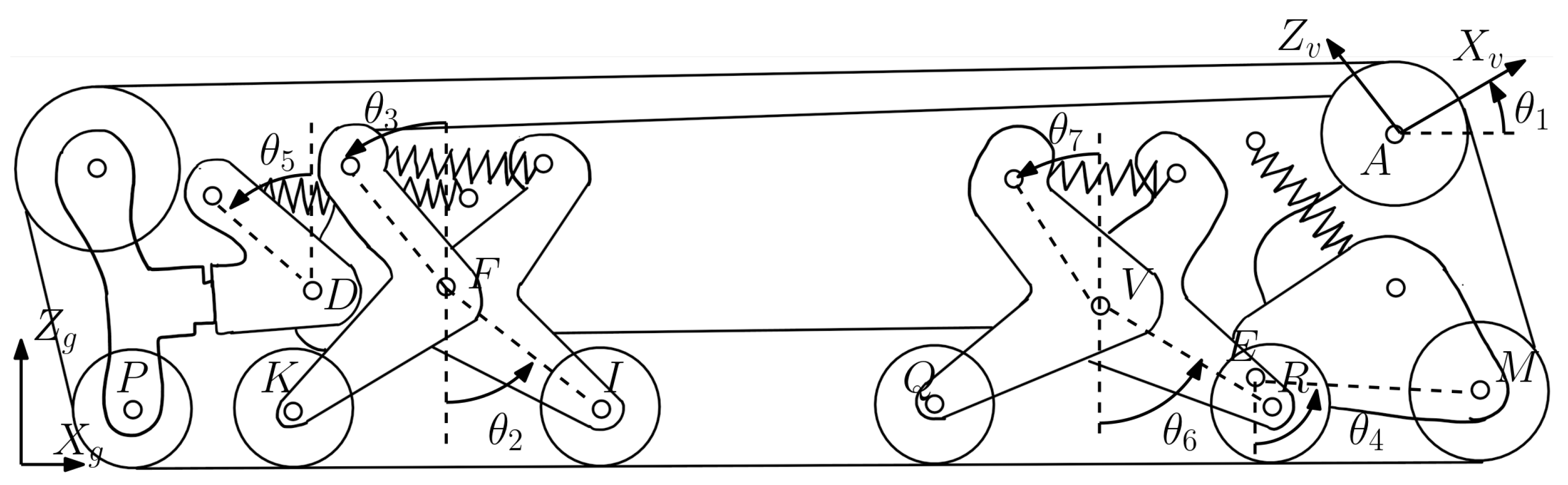
A global reference frame $X_g{Y}_g{Z}_g$ and a vehicle reference frame $X_v{Y}_v{Z}_v$ are defined in Figure 2. For simplicity, we assume a half-symmetry model. In this case, the $X_g-Z_g$ plane contains the vehicle center of mass. The model does not include roll and yaw rotations ($\phi$ and $\psi$) but only pitch movements ($\theta$).

Moreover, in the model, it is assumed that the wheels touch the surface at their lowest point and that the normal forces pass through the center of them. In fact, the goal of the created analytical approach is to compute the quasi-static kinematic model of the suspension to solve inverse kinematic problems. This means figuring out how the robot is set up based on where the wheels touch the ground.

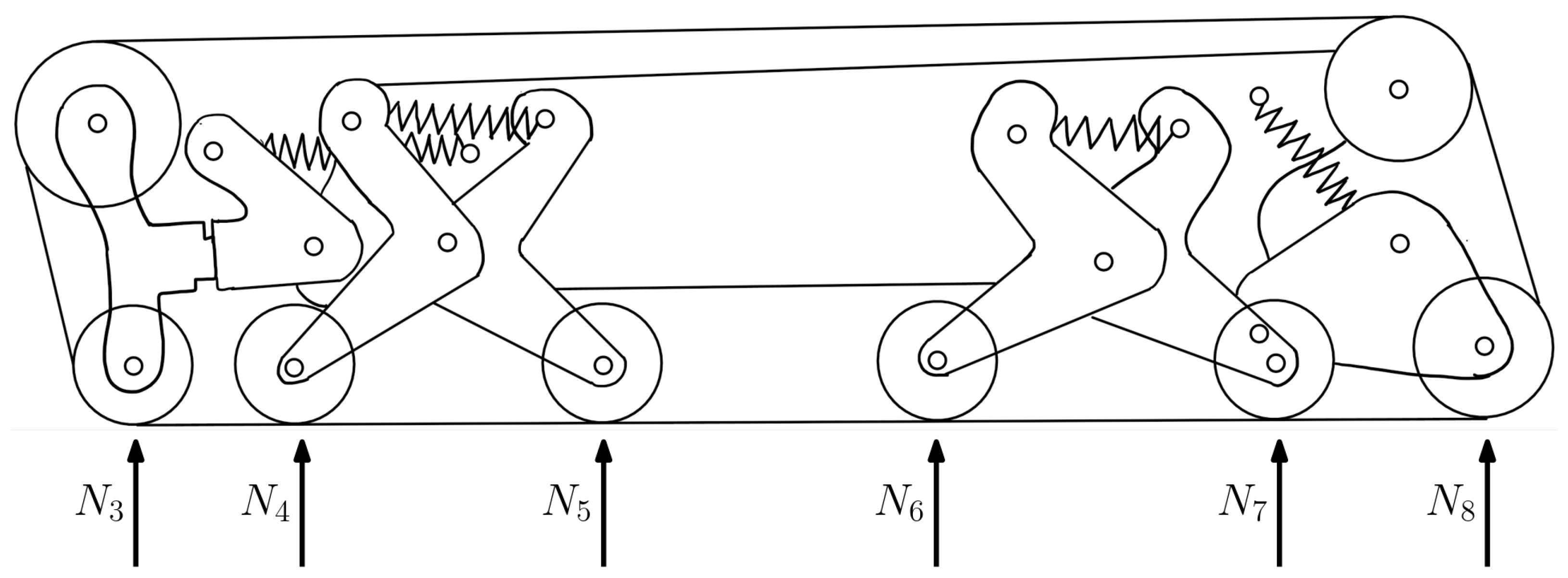
The system in Figure 2 consists of seven rigid bodies (six are the suspension elements, and the seventh rigid body is the vehicle frame) connected by four revolute joints located at the D, F, V, and E points.

Table 2. Degrees of freedom of the system (please refer to Figure 2).

Number	Description	Symbol
1	Vertical position of A (global ref. frame)	$x_A$
2	Horizontal position of A (global ref. frame)	$y_A$
3	Pitch of SF (robot’s pitch)	${\theta }_1$
4	Orientation of BFR relative to joint F	${\theta }_2$
5	Orientation of BFF relative to joint F	${\theta }_3$
6	Orientation of RSA relative to joint E	${\theta }_4$
7	Orientation of FSA relative to joint D	${\theta }_5$
8	Orientation of BRR relative to joint V	${\theta }_6$
9	Orientation of BRF relative to joint V	${\theta }_7$

reports the resulting nine DOFs.

3.2. Constraints

The support surface elevation map can be represented by the following expression:

$$Z=f_{te}\left(X\right)$$

(1)

where $f_{te}$ is a function that gives the height of the support surface $\left(Z\right)$ for any value of X.

Referring to the schematics of Figure 2, if we know where the first point of contact is on the X-axis and imagine that the wheels touch the ground at their lowest point, we can use these equations to describe how they are connected:

$$\begin{array}{c}{X}_P=X_{CP3}\end{array}$$

(2)

$$\begin{array}{c}{Z}_P-r_3=f_{te}\left(X_P\right)\end{array}$$

(3)

$$\begin{array}{c}{Z}_K-r_4=f_{te}\left(X_K\right)\end{array}$$

(4)

$$\begin{array}{c}{Z}_I-r_5=f_{te}\left(X_I\right)\end{array}$$

(5)

$$\begin{array}{c}{Z}_Q-r_6=f_{te}\left(X_Q\right)\end{array}$$

(6)

$$\begin{array}{c}{Z}_R-r_7=f_{te}\left(X_R\right)\end{array}$$

(7)

$$\begin{array}{c}{Z}_M-r_8=f_{te}\left(X_M\right)\end{array}$$

(8)

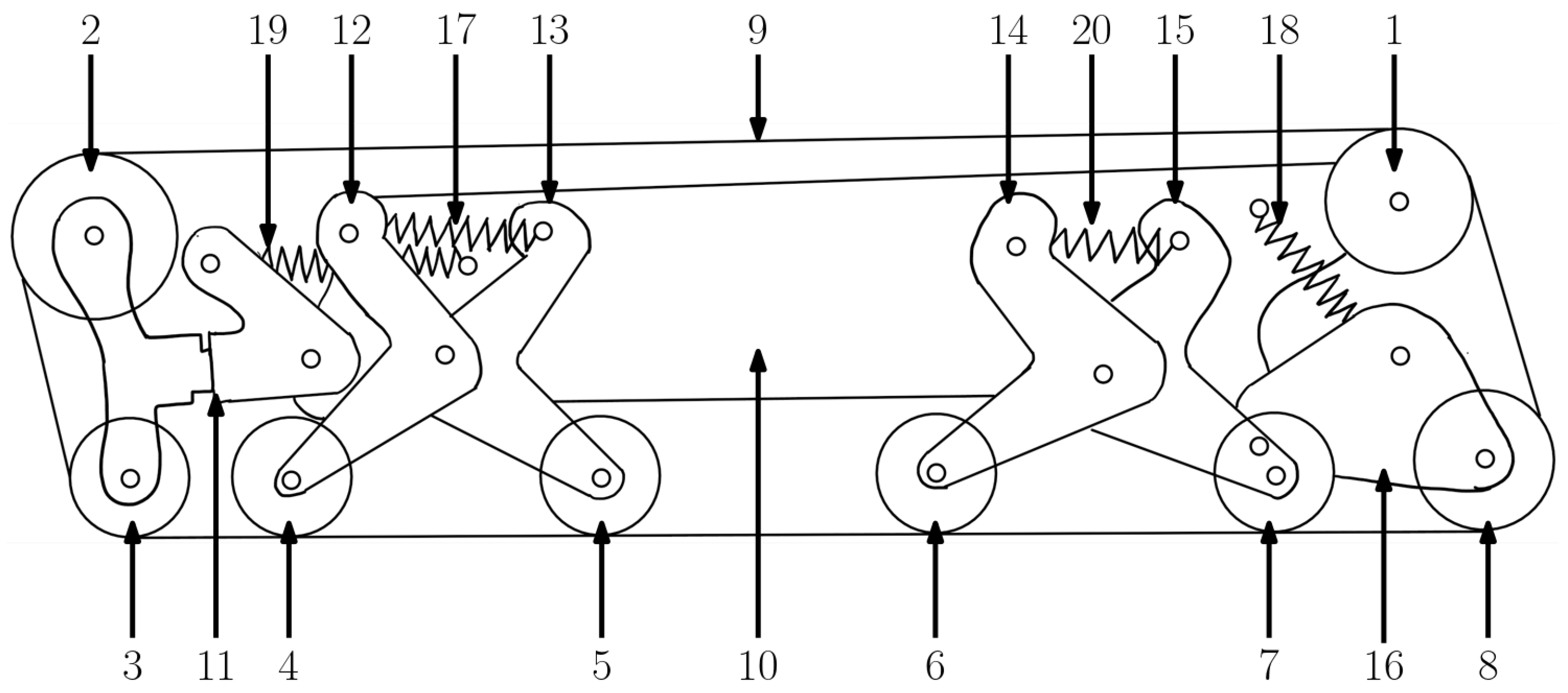
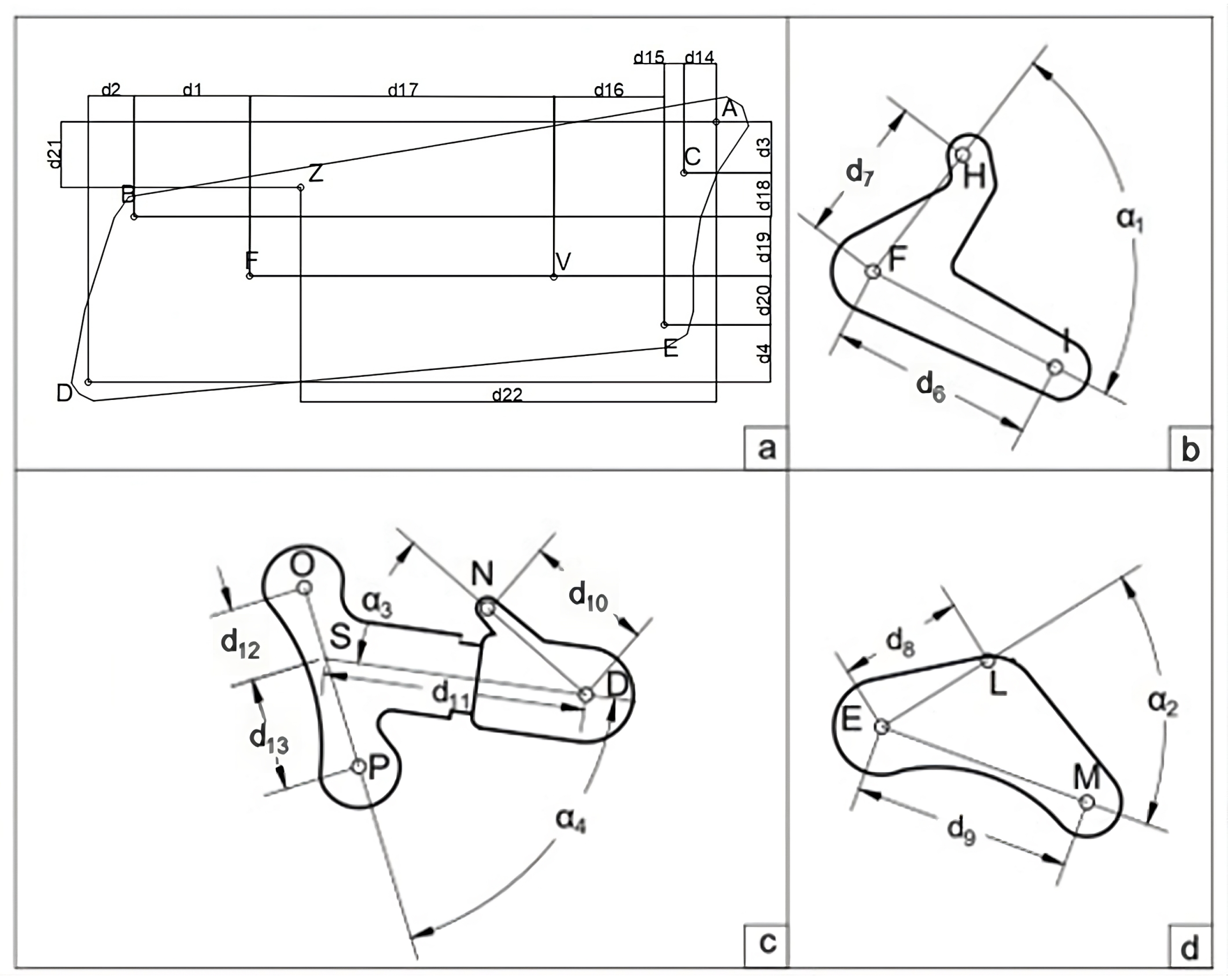
where $r_i$ is the radius of wheel i. Given the geometry of the suspension (Figure 1), the coordinates of the wheel centers (P, K, I, Q, R, and M) can be expressed in the vehicle reference system as a function of the DOFs in Table 2. For clarity, these equations are not reported here and are shown in Appendix A.

The track adds a kinematic constraint equation to the problem. Infinitely high stiffness and a negligible thickness characterize the track in this model. Under these assumptions, a change in the orientation of only one of the rigid bodies would change the length of the track. This constraint can be expressed as follows:

$$L_{track}=L_{nom}$$

(9)

where $L_{nom}$ is a design variable. Since the total length of the robot is approximately 1200 mm, the $L_{nom}$ imposed is 2845 mm. The derivation of the $L_{track}$ in terms of DOFs is explained in Appendix B.

Equations (2)–(9) represent a system of eight equations with nine unknowns corresponding to the system’s DOFs. Then, there are many different solutions to the problem, and we need to think about how things balance to find the right one. We will learn more about this in the next part.

3.3. Equilibrium Equations

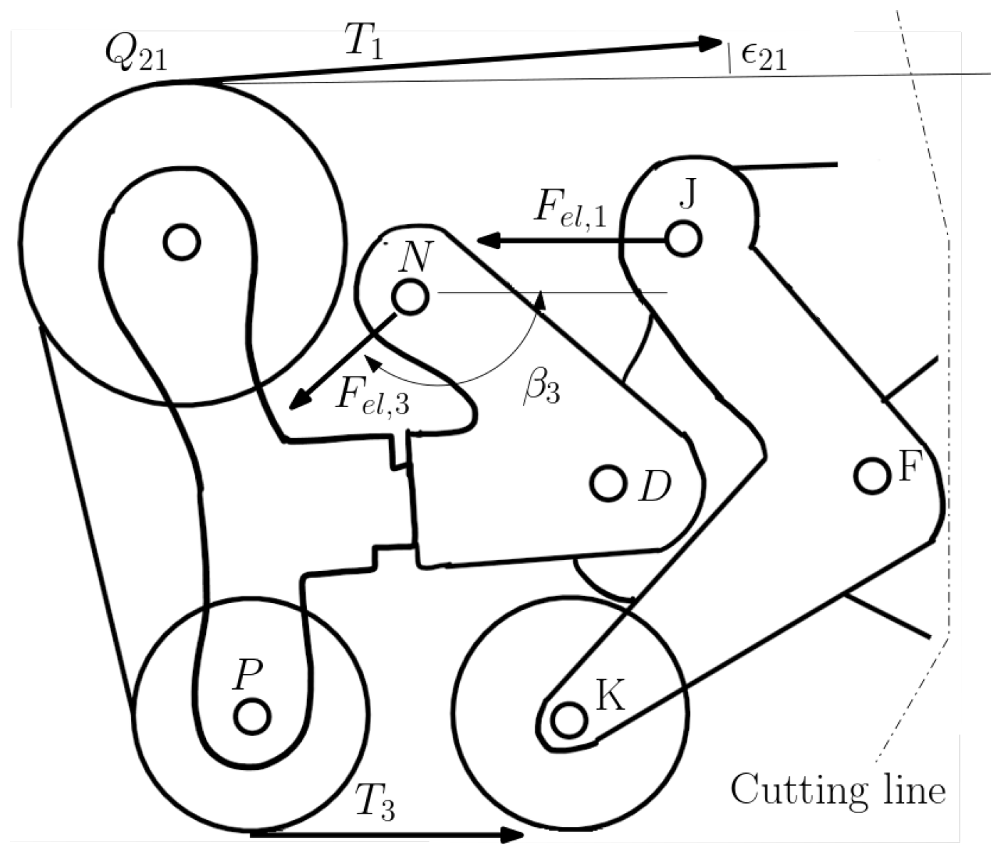
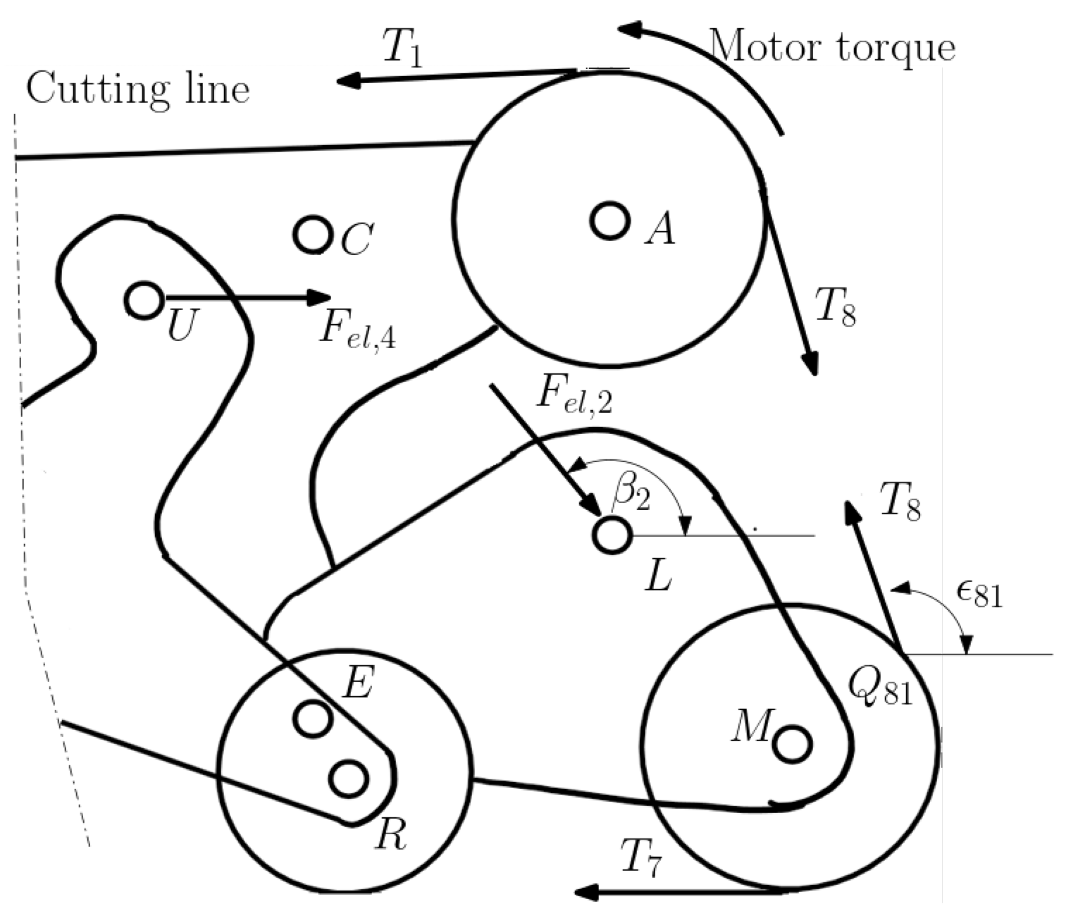
If a vehicle has more than two wheels, it becomes harder to figure out how much weight is on each wheel using normal equations. So, we need to look at how the elastic parts of the wheels bend to figure out how much weight they are carrying. To achieve this, we also need to think about how the bodies 2 to 7 of the vehicle balance and rotate with respect to D, F, V, and E. These equations introduce eighteen additional unknown parameters, which are reported in

Table 3. List of unknowns.

Unknowns	Description
$T_1$	Track tension of branch 1
$T_2$	Track tension of branch 2
$T_3$	Track tension of branch 3
$T_4$	Track tension of branch 4
$T_5$	Track tension of branch 5
$T_6$	Track tension of branch 6
$T_7$	Track tension of branch 7
$T_8$	Track tension of branch 8
C	Torque applied to W1 (A point)
$N_3$	Vertical force for wheel 3
$N_4$	Vertical force for wheel 4
$N_5$	Vertical force for wheel 5
$N_6$	Vertical force for wheel 6
$N_7$	Vertical force for wheel 7
$N_8$	Vertical force for wheel 8
$F_{el,1}$	Applied force to spring 1
$F_{el,2}$	Applied force to spring 2
$F_{el,3}$	Applied force to spring 3
$F_{el,4}$	Applied force to spring 4

.

The numbering of the track branch tensions is omitted for brevity. The weight of the single suspension bodies, wheels, and track is neglected. The half-vehicle mass is set to 110 kg, and the weight force applied to the vehicle’s center of gravity (COG) is indicated as W. The COG position ($X_G,Z_G$) has been defined in the center line of the vehicle. 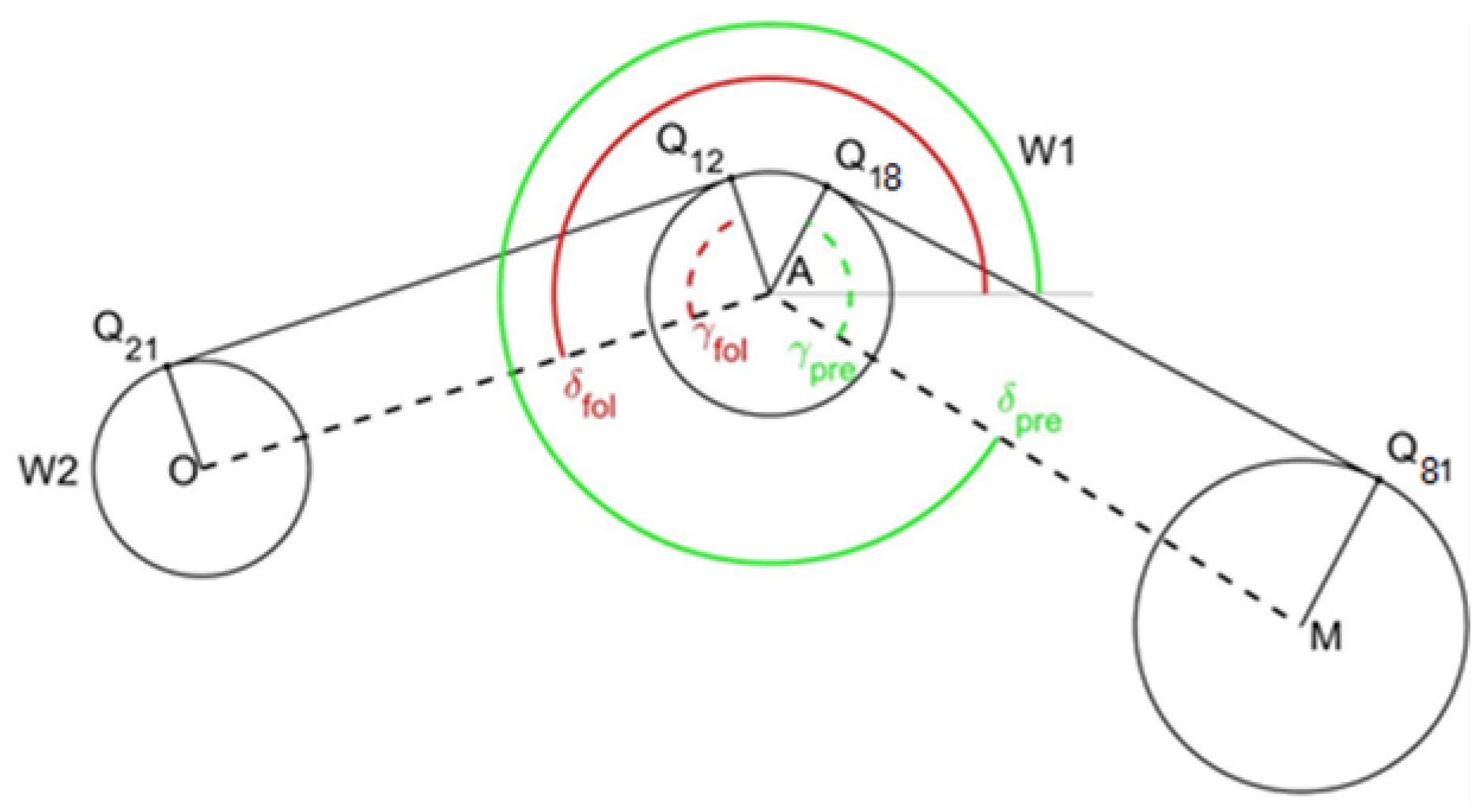The equilibrium equations are obtained and reported in Appendix C. The track tension directions relative to the horizontal direction (${ϵ}_{ij}$ and ${ϵ}_{ij}$) and the tangency point positions ($XQij$ and $ZQij$) are derived in Appendix B. Referring to Table 2, it is possible to express the rotation of the elastic forces (${\beta }_1,{\beta }_2,{\beta }_3$ and ${\beta }_4$) in terms of the system DOFs.

Elastic element deflection is used to compute forces $F_{el,1}$, $F_{el,2}$, $F_{el,3}$, and $F_{el,4}$. Each spring in the suspension has a set amount of pressure called pre-load. If a force smaller than the pre-load is applied to the spring, it will act like a stiff object and not bend or move. This applies to all four parts of the suspension that help the car move smoothly:

$$L_i=\left\{\begin{array}{cc}{L}_{max,i}\hfill & \mathrm{if}{F}_{el,i}<F_{pre,i}\hfill \\ L_{max,i}-(F_{el,i}-F_{pre,i})/k_i\hfill & \mathrm{otherwise}\hfill \end{array}\right.$$

(10)

where $L_i$ is the length of spring i when a force $F_{el,i}$ is applied to its ends, $F_{pre,i}$ and $L_{max,i}$ are the pre-load and the maximum length of spring i, respectively, and k is the elastic stiffness.

The DOFs in Appendix D are used to compute the deformable element lengths ($L_i$ for i = 1, 2, 3, 4). Wheel equilibrium equations are considered to close the system. $W_1$ is the only wheel with drive torque. This results in a further eight equations as follows. This simplifies the problem because, due to the tangential forces between the track and the support surface, the horizontal component of tension may vary along the track.

$$\begin{array}{c}{T}_1=T_2\end{array}$$

(11)

$$\begin{array}{c}{T}_2=T_3\end{array}$$

(12)

$$\begin{array}{c}{T}_3=T_4\end{array}$$

(13)

$$\begin{array}{c}{T}_4=T_5\end{array}$$

(14)

$$\begin{array}{c}{T}_5=T_6\end{array}$$

(15)

$$\begin{array}{c}{T}_6=T_7\end{array}$$

(16)

$$\begin{array}{c}{T}_7=T_8\end{array}$$

(17)

$$\begin{array}{c}{T}_8=T_1+C/r_1\end{array}$$

(18)

Equations (2)–(18) represent a system of twenty-eight equations in twenty-eight unknowns, which are the nine DOFs in Table 2 plus the nineteen unknown forces in Table 3.

4. Matlab^® R2023b Simulation Model

The analytical model just presented is implemented in Matlab^® R2023b software to evaluate the way the robot is positioned, the configuration of its suspension system, the external forces, and the forces acting on bodies when the “XXbot” overcomes a series of stair steps starting from a flat surface. Step dimensions have a height of 140 mm and a depth of 250 mm.

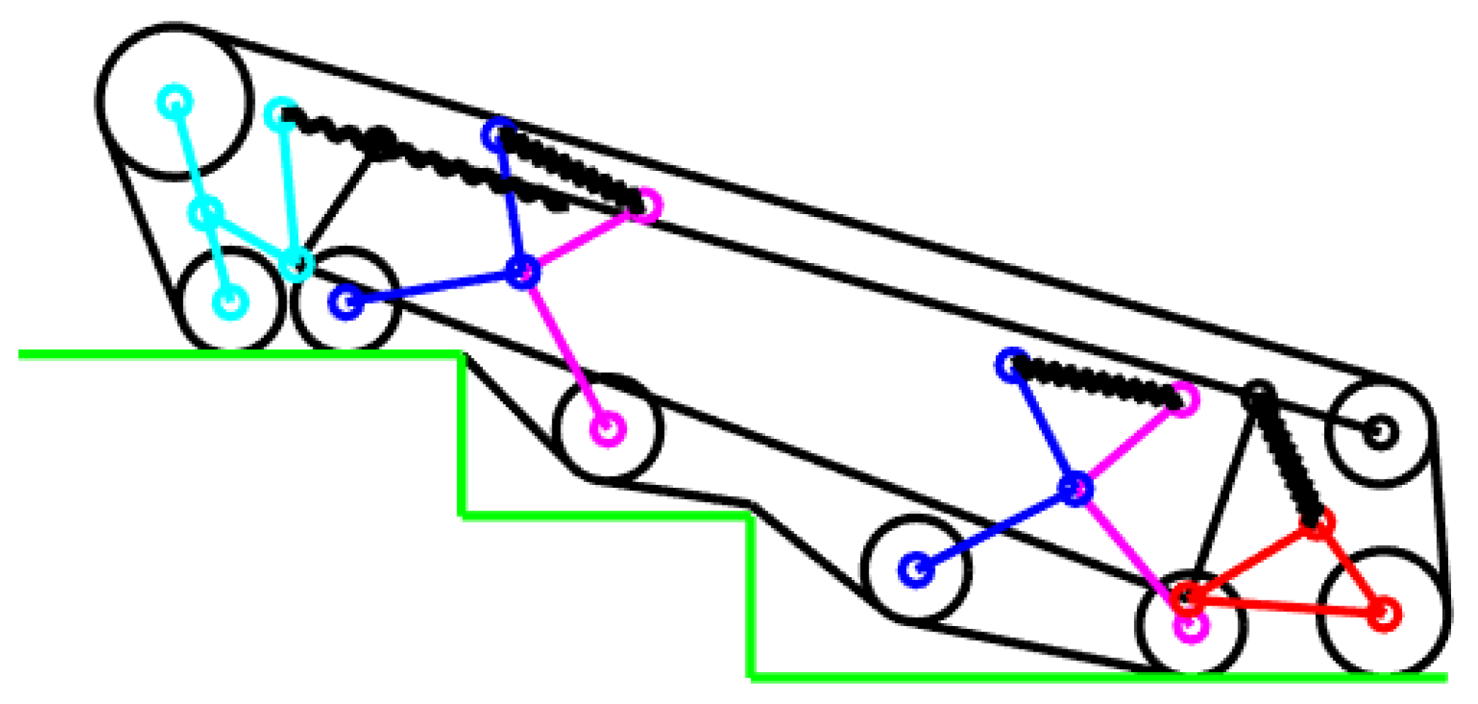
Since we are considering a quasi-static kinematic problem, the analytical model evaluates the static equilibrium of the robot in precise configurations. Since it is impossible to evaluate all the configurations that the robot assumes when climbing the flight of stairs, only the most significant ones are chosen. For clarity, Figure 3 shows the configuration where wheels $W_3$ and $W_4$ are on the second step. When an edge of the step is located between two wheels and deforms the shape of the track, it is necessary to evaluate the constraining reaction $N_{Ci}$ that the corner applies to the robot. For simplicity, it is considered vertical and applied at the step edge. This leads to the introduction of two further unknowns to the problem, the vertical reaction $N_{Ci}$ and the track tension $T_{Ci}$ downstream of the corner. $T_{prev}$ is the track tension in the upstream branch of the corner. To close the system, two further equations that evaluate the equilibrium of a little portion of the track around the obstacle are used:

$$\begin{array}{c}{T}_{prev}\sin \left({ϵ}_{Ci-W_{prev}}\right)+T_{Ci}\sin \left({ϵ}_{Ci-W_{succ}}\right)=N_{Ci}\end{array}$$

(19)

$$\begin{array}{c}{T}_{prev}\cos \left({ϵ}_{Ci-W_{prev}}\right)+T_{Ci}\cos \left({ϵ}_{Ci-W_{succ}}\right)=0\end{array}$$

(20)

Furthermore, the vertical constraining reaction $N_{Ci}$ is taken into account in the equilibrium equations of the vertical translation and rotation around the point P as follows:

$$W=N_3+N_4+N_5+N_6+N_7+N_8+N_{Ci}$$

(21)

$$\begin{array}{c}{N}_4(X_K-X_P)+N_5(X_I-X_P)+N_6(X_Q-X_P)+N_7(X_R-X_P)\hfill \\ +N_8(X_M-X_P)+N_{Ci}(X_{NCi}-X_P)=W(X_G-X_P)\hfill \end{array}$$

(22)

This procedure is repeated as many times as there are step edges deforming the shape of the track in a configuration.

5. MSC Adams ATV Simulations

MSC.ADAMS 2019.2 software performs the dynamical simulation of mechanical systems. It is like a box that has important parts and extra parts that can be added. The ADAMS/View package helps us to understand how mechanical systems work. There are other packages that focus on different parts of machines. Tracked vehicles can be modeled using the ADAMS Tracked Vehicle (ATV) Toolkit.

It allows creating, modifying, and simulating realistic spatial models for tracked vehicles in the ADAMS environment. Using this software, a dynamic simulation of a stair-climbing case is carried out. For simplicity, a half-symmetry model is assumed for the vehicle. Also in this case, the $X_g-Z_g$ plane, defined in Section 3.1, contains the vehicle center of mass. The model does not include roll and yaw rotations ($\phi$ and $\psi$) but only pitch movements ($\theta$). Robot-specific details and step dimensions are taken from the Matlab analytical model described above. The angular velocity of the sprocket is 15 deg/s. The half-vehicle mass is set to 110 kg.

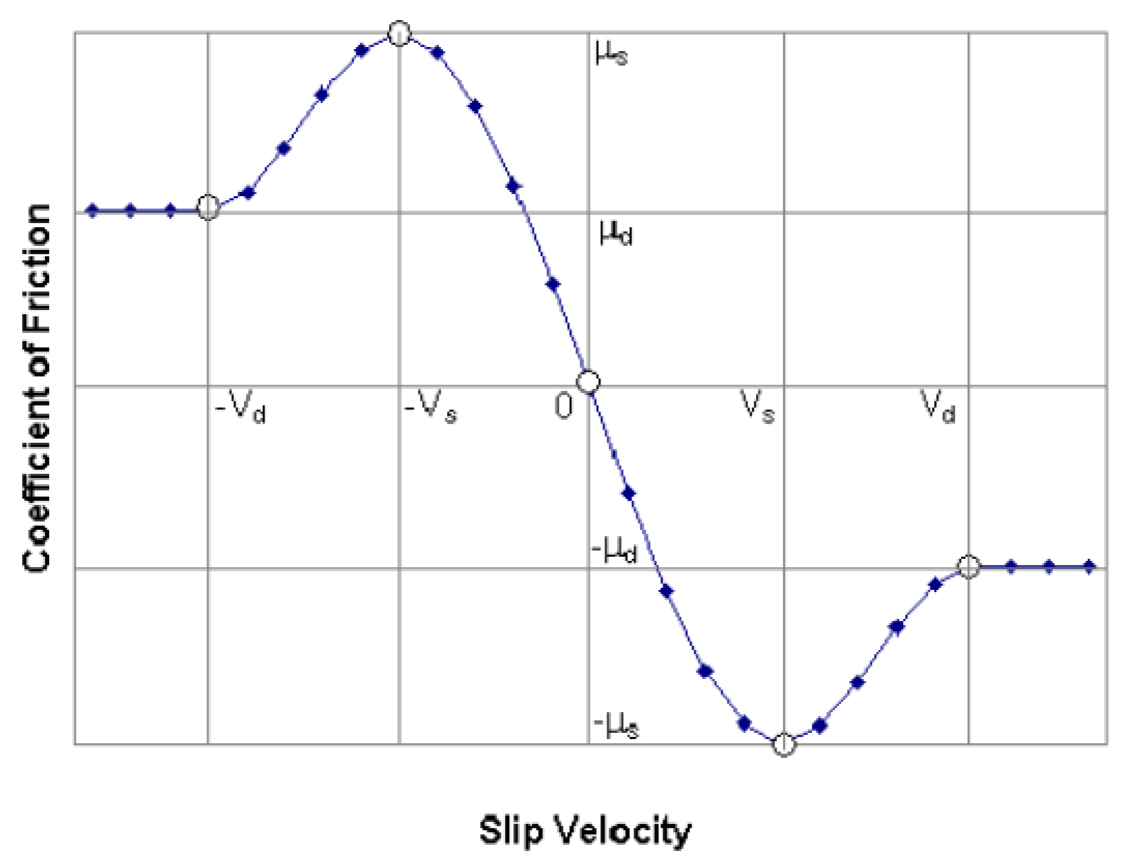
ADAMS uses a relatively simple velocity-based friction model for contacts. Figure 4 shows the dependence between the coefficient of friction and the slip velocity. $V_s$, the stiction transition velocity, is the velocity at which the coefficient of friction achieves a maximum value of ${\mu }_S$. ${\mu }_S$ is the coefficient of static friction between the track and the ground. The coefficient of dynamic friction between the track and the ground is ${\mu }_D$. ADAMS changes ${\mu }_S$ to ${\mu }_D$ as the slip velocity at the contact point increases. When the slip velocity reaches the value of $V_D$, the effective coefficient of friction is equal to the dynamic coefficient ${\mu }_D$.

Table 4. List of unknowns.

Name	Description	Value
${\mu }_S$	static friction coefficient	0.9
${\mu }_D$	dynamic friction coefficient	0.7
$V_S$	stiction transition velocity	0.001 m/s
$V_D$	friction transition velocity	0.05 m/s

summarizes contact parameter values.

The case of the stair-climbing simulations is described in the following. First, the tracked robot model and the stair-shaped ground were created in the pre-processing environment of the Adams ATV software. Then, the simulation parameters were defined, and the calculation was launched in the solution environment. The program initially solves the static problem in the initial condition. It then solves the dynamic problem for each time instant until it reaches the end of the simulation. The simulation results are reported in the software post-processing environment.

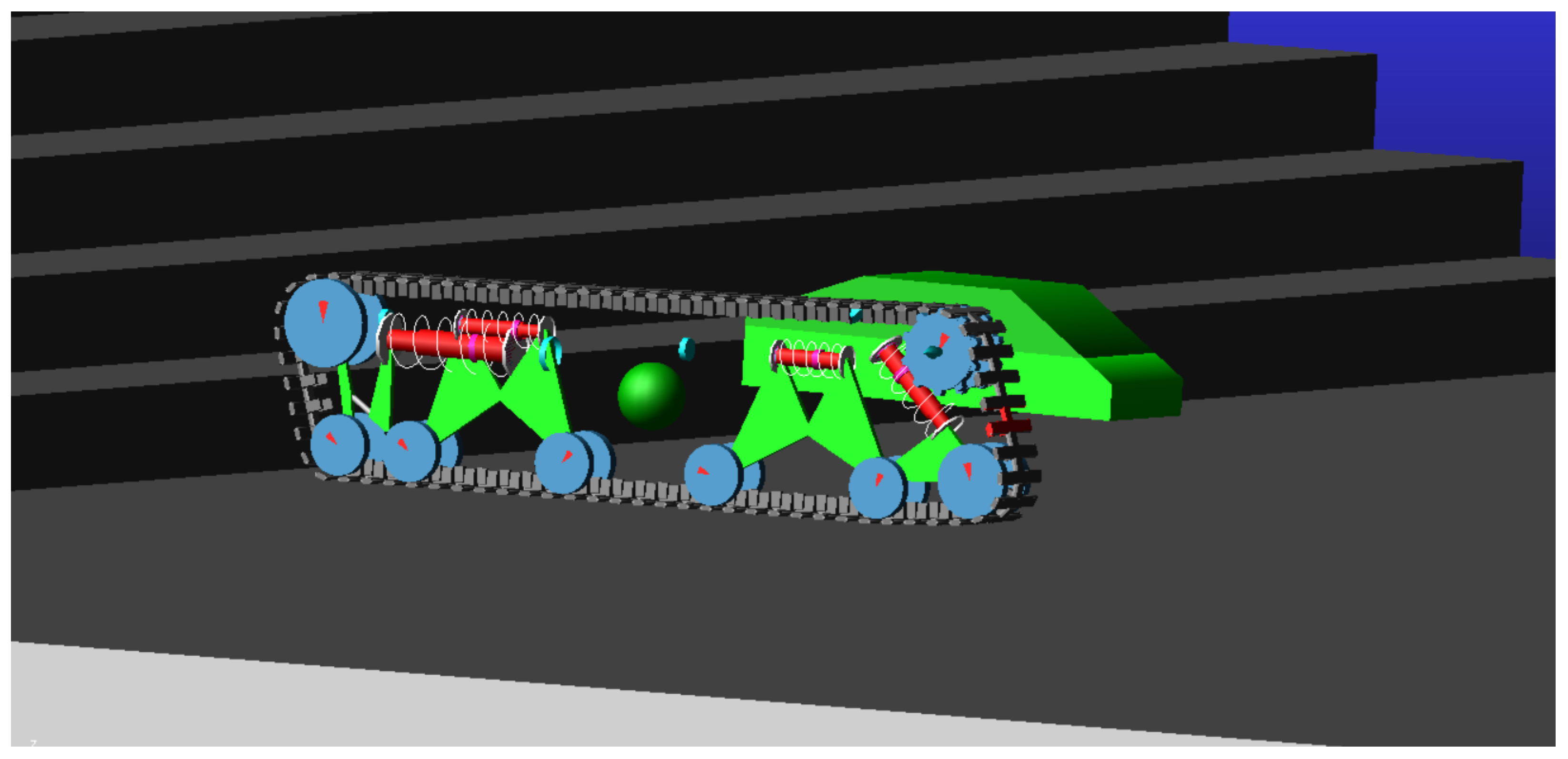
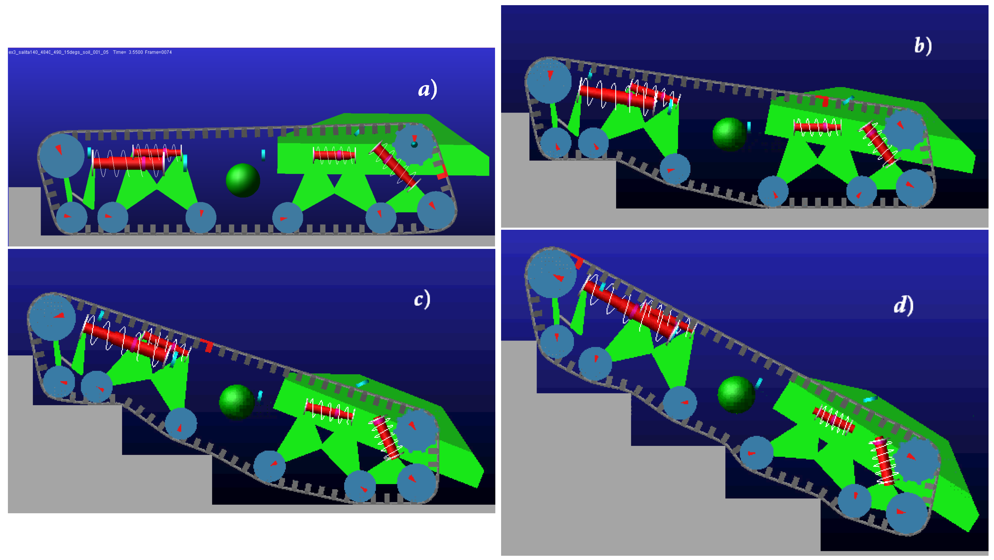
Figure 5 shows the simulation’s initial conditions in a perspective view. Figure 6 shows a sequence of simulation snapshots in the moments of time that seemed most significant to us. The following table summarizes the forces in the spring elements, the vertical contact forces between the track and step, as well as the tension in the belt downstream and upstream of the sprocket for the same instants of simulation time.

Table 5. Forces in the spring elements, the vertical contact forces between track and step, and belt tension for flat ground configuration.

Name	Description	Value (N)
$F_{el,1}$	Applied force to spring 1	265
$F_{el,2}$	Applied force to spring 2	778
$F_{el,3}$	Applied force to spring 3	691
$F_{el,4}$	Applied force to spring 4	401
$N_3$	Vertical force for wheel 3	84
$N_4$	Vertical force for wheel 4	240
$N_5$	Vertical force for wheel 5	190
$N_6$	Vertical force for wheel 6	297
$N_7$	Vertical force for wheel 7	279
$N_8$	Vertical force for wheel 8	0
$T_{up}$	Belt tension upstream of the sprocket	613
$T_{down}$	Belt tension downstream of the sprocket	641

refers to Figure 6a (flat ground).

Table 6. Forces in the spring elements, the vertical contact forces between track and step, and belt tension for first step configuration.

Name	Description	Value (N)
$F_{el,1}$	Applied force to spring 1	219
$F_{el,2}$	Applied force to spring 2	1105
$F_{el,3}$	Applied force to spring 3	607
$F_{el,4}$	Applied force to spring 4	268
$N_3$	Vertical force for wheel 3	138
$N_4$	Vertical force for wheel 4	112
$N_5$	Vertical force for wheel 5	0
$N_6$	Vertical force for wheel 6	88
$N_7$	Vertical force for wheel 7	198
$N_8$	Vertical force for wheel 8	221
$N_{C1}$	Vertical contact forces between track and step 1	332
$T_{up}$	Belt tension upstream of the sprocket	500
$T_{down}$	Belt tension downstream of the sprocket	653

refers to Figure 6b (first step).

Table 7. Forces in the spring elements, the vertical contact forces between track and step, and belt tension for second step configuration.

Name	Description	Value (N)
$F_{el,1}$	Applied force to spring 1	284
$F_{el,2}$	Applied force to spring 2	1418
$F_{el,3}$	Applied force to spring 3	469
$F_{el,4}$	Applied force to spring 4	296
$N_3$	Vertical force for wheel 3	0
$N_4$	Vertical force for wheel 4	56
$N_5$	Vertical force for wheel 5	0
$N_6$	Vertical force for wheel 6	0
$N_7$	Vertical force for wheel 7	95
$N_8$	Vertical force for wheel 8	310
$N_{C1}$	Vertical contact forces between track and step 1	88
$N_{C2}$	Vertical contact forces between track and step 2	570
$T_{up}$	Belt tension upstream of the sprocket	558
$T_{down}$	Belt tension downstream of the sprocket	779

refers to Figure 6c (second step).

Table 8. Forces in the spring elements, the vertical contact forces between track and step, and belt tension for third step configuration.

Name	Description	Value (N)
$F_{el,1}$	Applied force to spring 1	199
$F_{el,2}$	Applied force to spring 2	1467
$F_{el,3}$	Applied force to spring 3	347
$F_{el,4}$	Applied force to spring 4	560
$N_3$	Vertical force for wheel 3	0
$N_4$	Vertical force for wheel 4	0
$N_5$	Vertical force for wheel 5	0
$N_6$	Vertical force for wheel 6	0
$N_7$	Vertical force for wheel 7	0
$N_8$	Vertical force for wheel 8	0
$N_{C1}$	Vertical contact forces between track and step 1	383
$N_{C2}$	Vertical contact forces between track and step 2	450
$N_{C3}$	Vertical contact forces between track and step 3	283
$T_{up}$	Belt tension upstream of the sprocket	448
$T_{down}$	Belt tension downstream of the sprocket	1120

refers to Figure 6d (third step).

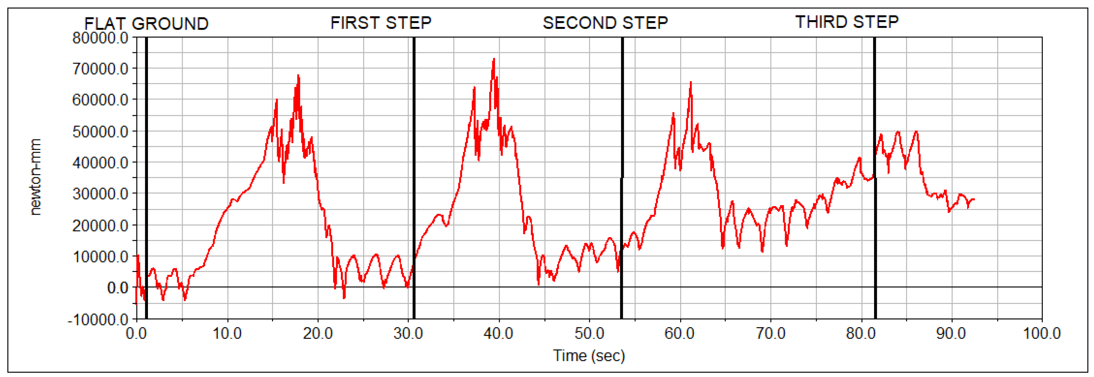
Finally, Figure 7 shows the motor torque during the stair-climbing simulation. Vertical lines named flat ground, first step, second step, and third step refer to the simulation instants shown in Figure 6. It can be seen that maximum torque occurs when the front of the robot meets the step and overcomes it.

The MSC.ADAMS simulation is proof that the proposed tracked robot can effectively climb a flight of stairs without tipping over backwards.

6. Conclusions and Future Work

This paper talks about a new track-based robot called “XXbot”. It uses an innovative system of articulated suspension. Each wheel on the road can move up and down to adapt the track shape to the stair structure. The developed design aims to perform better compared to other stair-climbing robots. We also developed a special model that helps us to figure out how the robot will move according to the shape of the ground. The model uses a static approach of forces and consists of 28 equations in 28 unknowns that are the nine suspension DOFs and the nineteen unknown forces, including internal and contact forces. This means that we are trying to figure out how the rover is positioned on the ground and how its wheels are set up while also considering that the track on the wheels cannot change its length. It is a useful tool to predict the behavior of the system in stair-climbing conditions. The novelty of the present work, compared to [33], is that the model has been modified to be used as a tool to design new complex systems and optimize the performance of the new robots. To verify that the proposed tracked robot can effectively climb a flight of stairs without tipping over backwards, an MSC.ADAMS dynamic simulation was carried out. The angular velocity of the sprocket was 15 deg/s. The half-vehicle mass was set to 110 kg. Figure 6 and Table 5, Table 6, Table 7 and Table 8 summarize the simulation results and prove the effectiveness of the proposed vehicle.

Given the vehicle’s excellent ability to overcome a flight of stairs, it could be used in hazardous work environments and in repetitive tasks. Specifically, it can be used for surveillance and monitoring, military, health care, industrial, and agricultural applications. In particular, it can be utilized for the inspection and monitoring of buildings and infrastructure, including commercial and residential buildings.

Nonetheless, the proposed platform could be used as a starting point to build an electric-powered wheelchair (EPW) and help people with disabilities overcome architectural barriers.

References

1. Bruzzone, L.E.; Quaglia, G. Review article: Locomotion systems for ground mobile robots in unstructured environments. Mech. Sci. 2012, 3, 49–62. [Google Scholar] [CrossRef]
2. Reina, G.; Foglia, M. On the mobility of all-terrain rovers. Ind. Robot 2013, 40, 121–131. [Google Scholar] [CrossRef]
3. Uchida, Y.; Furuichi, K.; Hirose, S. Fundamental performance of a 6 wheeled off-road vehicle “HELIOS-V”. In Proceedings of the 1999 IEEE International Conference on Robotics and Automation (Cat. No. 99CH36288C), Detroit, MI, USA, 10–15 May 1999; Volume 3, pp. 2336–2341. [Google Scholar] [CrossRef]
4. Takaki, T.; Aoyama, T.; Ishii, I. Development of inverted pendulum robot capable of climbing stairs using planetary wheel mechanism. In Proceedings of the 2013 IEEE International Conference on Robotics and Automation, Karlsruhe, Germany, 6–10 May 2013; pp. 5618–5624. [Google Scholar] [CrossRef]
5. Mostýn, V.; Krys, V.; Kot, T.; Bobovský, Z.; Novak, P. The synthesis of a segmented stair-climbing wheel. Int. J. Adv. Robot. Syst. 2018, 15, 172988141774947. [Google Scholar] [CrossRef]
6. Kim, D.; Hong, H.; Kim, H.S.; Kim, J. Optimal design and kinetic analysis of a stair-climbing mobile robot with rocker-bogie mechanism. Mech. Mach. Theory 2012, 50, 90–108. [Google Scholar] [CrossRef]
7. Yoneda, K.; Ota, Y.; Hirose, S. High-grip Stair Climber with Powder-filled Belts. Int. J. Robot. Res. 2009, 28, 81–89. [Google Scholar] [CrossRef]
8. Bruzzone, L.; Nodehi, S.E.; Fanghella, P. Tracked Locomotion Systems for Ground Mobile Robots: A Review. Machines 2022, 10, 648. [Google Scholar] [CrossRef]
9. Lee, W.; Kang, S.; Kim, M.; Park, M. ROBHAZ-DT3: Teleoperated mobile platform with passively adaptive double-track for hazardous environment applications. In Proceedings of the 2004 IEEE/RSJ International Conference on Intelligent Robots and Systems (IROS) (IEEE Cat. No. 04CH37566), Sendai, Japan, 28 September–2 October 2004; Volume 1, pp. 33–38. [Google Scholar] [CrossRef]
10. Hirose, S.; Sensu, T. The TAQT Carrier: A Practical Terrain Adaptive Quadru-track Carrier Robot. In Proceedings of the IEEE/RSJ International Conference on Intelligent Robots and Systems, Raleigh, NC, USA, 7–10 July 1992; Volume 3, pp. 2068–2073. [Google Scholar] [CrossRef]
11. Moosavian, S.A.A.; Semsarilar, H.; Kalantari, A. Design and Manufacturing of a Mobile Rescue Robot. In Proceedings of the 2006 IEEE/RSJ International Conference on Intelligent Robots and Systems, Beijing, China, 9–15 October 2006; pp. 3982–3987. [Google Scholar] [CrossRef]
12. Vu, Q.H.; Kim, B.S.; Song, J.B. Autonomous stair climbing algorithm for a small four-tracked robot. In Proceedings of the 2008 International Conference on Control, Automation and Systems, Seoul, Republic of Korea, 14–17 October 2008; pp. 2356–2360. [Google Scholar] [CrossRef]
13. Sugahara, Y.; Hashimoto, K.; Sunazuka, H.; Kawase, M.; Ohta, A.; Tanaka, C.; Lim, H.-O.; Takanishi, A. Towards the Biped Walking Wheelchair. In Proceedings of the First IEEE/RAS-EMBS International Conference on Biomedical Robotics and Biomechatronics, BioRob 2006, Pisa, Italy, 20–22 February; pp. 781–786. [CrossRef]
14. Lee, C.H.; Lee, K.M.; Yoo, J.; Kim, I.S.; Bang, Y.B. A compact stair-climbing wheelchair with two 3-DOF legs and a 1-DOF base. Ind. Robot 2016, 43, 181–192. [Google Scholar] [CrossRef]
15. Hutter, M.; Gehring, C.; Jud, D.; Lauber, A.; Bellicoso, C.D.; Tsounis, V.; Hwangbo, J.; Bodie, K.; Fankhauser, P.; Bloesch, M.; et al. ANYmal—A highly mobile and dynamic quadrupedal robot. In Proceedings of the 2016 IEEE/RSJ International Conference on Intelligent Robots and Systems (IROS), Daejeon, Republic of Korea, 9–14 October 2016; pp. 38–44. [Google Scholar] [CrossRef]
16. Moore, E.; Campbell, D.; Grimminger, F.; Buehler, M. Reliable stair climbing in the simple hexapod ‘RHex’. In Proceedings of the Proceedings 2002 IEEE International Conference on Robotics and Automation (Cat. No. 02CH37292), Washington, DC, USA, 11–15 May 2002; Volume 3, pp. 2222–2227. [Google Scholar] [CrossRef]
17. Ugenti, A.; Vulpi, F.; Domínguez, R.; Cordes, F.; Milella, A.; Reina, G. On the role of feature and signal selection for terrain learning in planetary exploration robots. J. Field Robot. 2022, 39, 355–370. [Google Scholar] [CrossRef]
18. Quaglia, G.; Butera, L.G.; Chiapello, E.; Bruzzone, L. UGV Epi.q-Mod. In Advances on Theory and Practice of Robots and Manipulators; Ceccarelli, M., Glazunov, V.A., Eds.; Springer: Cham, Switzerland, 2014; pp. 331–339. [Google Scholar]
19. Klemm, V.; Morra, A.; Salzmann, C.; Tschopp, F.; Bodie, K.; Gulich, L.; Küng, N.; Mannhart, D.; Pfister, C.; Vierneisel, M.; et al. Ascento: A Two-Wheeled Jumping Robot. In Proceedings of the 2019 International Conference on Robotics and Automation (ICRA), Montreal, QC, Canada, 20–24 May 2019; pp. 7515–7521. [Google Scholar]
20. Yuan, J.; Hirose, S. Research on leg-wheel hybrid stair-climbing robot, Zero Carrier. In Proceedings of the 2004 IEEE International Conference on Robotics and Biomimetics, Shenyang, China, 22–26 August 2004; pp. 654–659. [Google Scholar] [CrossRef]
21. Nakajima, S. Stair-climbing gait for a four-wheeled vehicle. Robomech J. 2020, 7, 20. [Google Scholar] [CrossRef]
22. Chocoteco, J.A.; Morales, R.; Feliu-Batlle, V. Enhancing the Trajectory Generation of a Stair-Climbing Mobility System. Sensors 2017, 17, 2608. [Google Scholar] [CrossRef]
23. Lawn, M.; Ishimatsu, T. Modeling of a stair-climbing wheelchair mechanism with high single-step capability. IEEE Trans. Neural Syst. Rehabil. Eng. 2003, 11, 323–332. [Google Scholar] [CrossRef] [PubMed]
24. Hirose, S.; Fukuda, Y.; Yoneda, K.; Nagakubo, A.; Tsukagoshi, H.; Arikawa, K.; Endo, G.; Doi, T.; Hodoshima, R. Quadruped walking robots at Tokyo Institute of Technology. IEEE Robot. Autom. Mag. 2009, 16, 104–114. [Google Scholar] [CrossRef]
25. Podobnik, J.; Rejc, J.; Slajpah, S.; Munih, M.; Mihelj, M. All-Terrain Wheelchair: Increasing Personal Mobility with a Powered Wheel-Track Hybrid Wheelchair. IEEE Robot. Autom. Mag. 2017, 24, 26–36. [Google Scholar] [CrossRef]
26. Hirose, S.; Fukushima, E.; Damoto, R.; Nakamoto, H. Design of terrain adaptive versatile crawler vehicle HELIOS-VI. In Proceedings of the Proceedings 2001 IEEE/RSJ International Conference on Intelligent Robots and Systems. Expanding the Societal Role of Robotics in the the Next Millennium (Cat. No. 01CH37180), Maui, HI, USA, 29 October–3 November 2001; Volume 3, pp. 1540–1545. [Google Scholar] [CrossRef]
27. Bruzzone, L.; Baggetta, M.; Nodehi, S.E.; Bilancia, P.; Fanghella, P. Functional Design of a Hybrid Leg-Wheel-Track Ground Mobile Robot. Machines 2021, 9, 10. [Google Scholar] [CrossRef]
28. Michaud, F.; Letourneau, D.; Arsenault, M.; Bergeron, Y.; Cadrin, R.; Gagnon, F.; Legault, M.A.; Millette, M.; Pare, J.F.; Tremblay, M.C.; et al. AZIMUT, a leg-track-wheel robot. In Proceedings of the 2003 IEEE/RSJ International Conference on Intelligent Robots and Systems (IROS 2003) (Cat. No. 03CH37453), Las Vegas, NV, USA, 27–31 October 2003; Volume 3, pp. 2553–2558. [Google Scholar] [CrossRef]
29. Quaglia, G.; Nisi, M. Design of a self-leveling cam mechanism for a stair climbing wheelchair. Mech. Mach. Theory 2017, 112, 84–104. [Google Scholar] [CrossRef]
30. Pappalettera, A.; Bottiglione, F.; Mantriota, G.; Reina, G. Watch the Next Step: A Comprehensive Survey of Stair-Climbing Vehicles. Robotics 2023, 12, 74. [Google Scholar] [CrossRef]
31. Li, Y.; Li, M.; Zhu, H.; Hu, E.; Tang, C.; Li, P.; You, S. Development and applications of rescue robots for explosion accidents in coal mines. J. Field Robot. 2019, 37, 466–489. [Google Scholar] [CrossRef]
32. Sun, B.; Jing, X. A tracked robot with novel bio-inspired passive “legs”. Robot. Biomim. 2017, 4, 18. [Google Scholar] [CrossRef] [PubMed]
33. Ugenti, A.; Galati, R.; Mantriota, G.; Reina, G. Analysis of an all-terrain tracked robot with innovative suspension system. Mech. Mach. Theory 2023, 182, 105237. [Google Scholar] [CrossRef]
Figure 1. XXbot robot concept. Please refer to Table 1 to numbers explanation.
Robotics 13 00045 g001
Figure 2. Reference frames and degrees of freedom.
Robotics 13 00045 g002
Figure 3. “XXbot” on the second stair step.
Robotics 13 00045 g003
Figure 4. Coefficient of friction varying with slip velocity.
Robotics 13 00045 g004
Figure 5. Tracked vehicle model in ATV Toolkit.
Robotics 13 00045 g005
Figure 6. ADAMS ATV stair-climbing simulation snapshots: (a) Top left = flat ground. (b) Top right = first step. (c) Bottom left = second step. (d) Bottom right = third step.
Robotics 13 00045 g006
Figure 7. Motor torque in the stair-climbing process.
Robotics 13 00045 g007