
Development of Local Path Planning Using Selective Model Predictive Control, Potential Fields, and Particle Swarm Optimization


Abstract
1. Introduction
2. Selective MPC-PF-PSO Algorithm
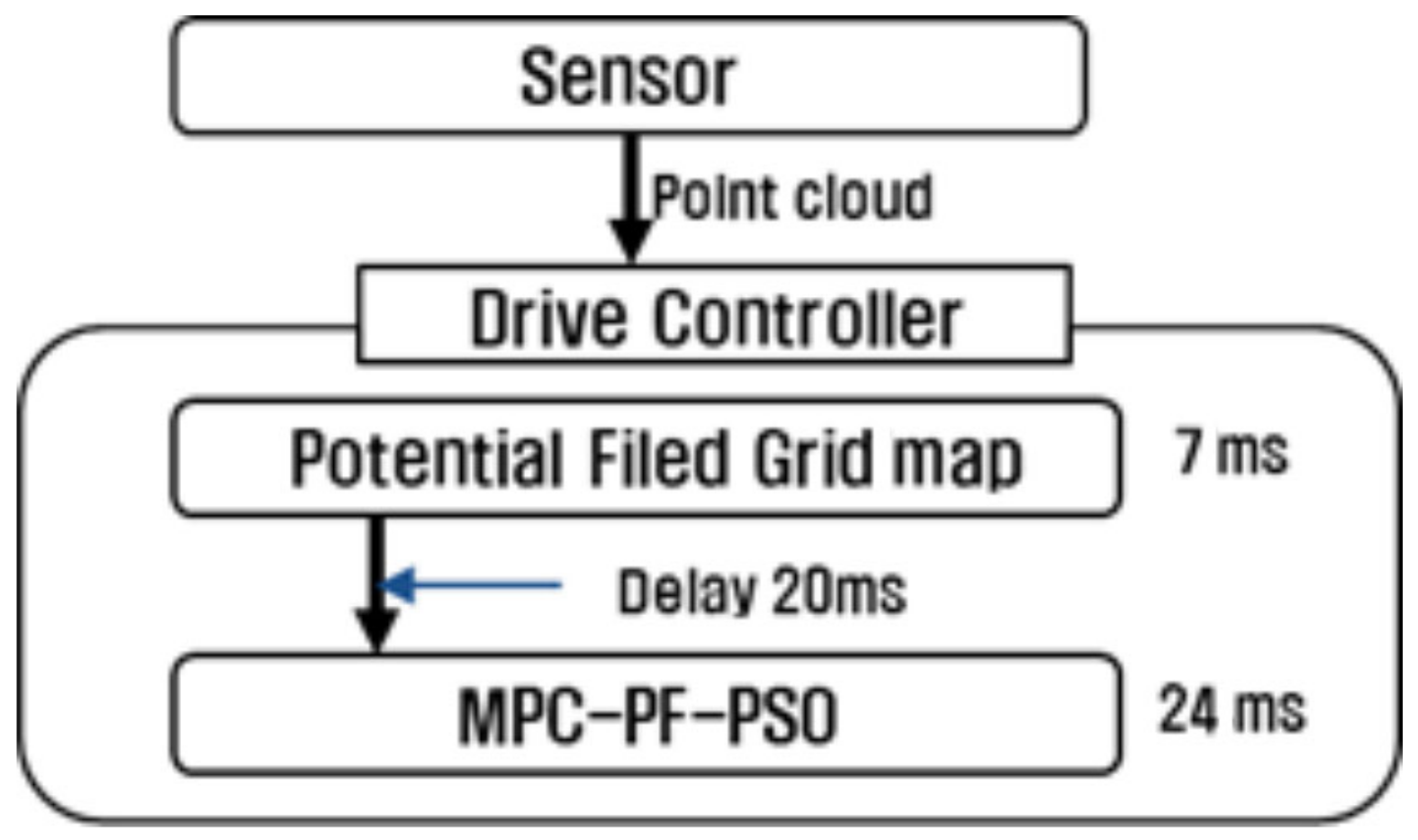
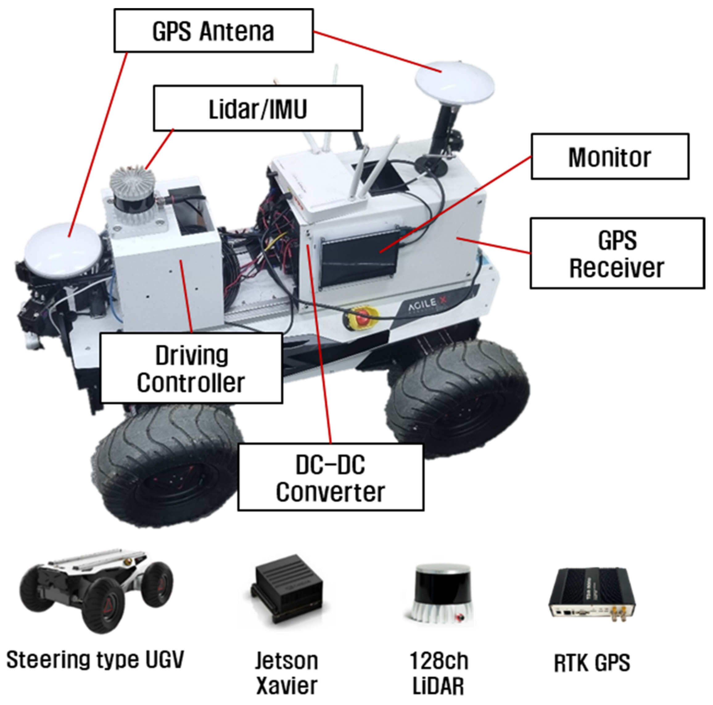
2.1. System Configuration
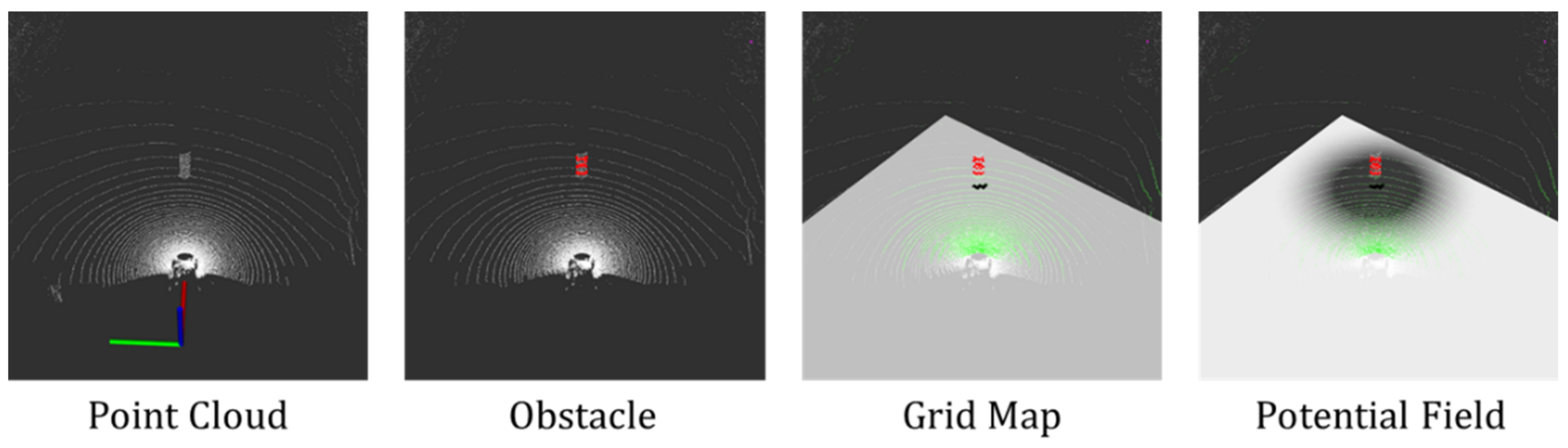
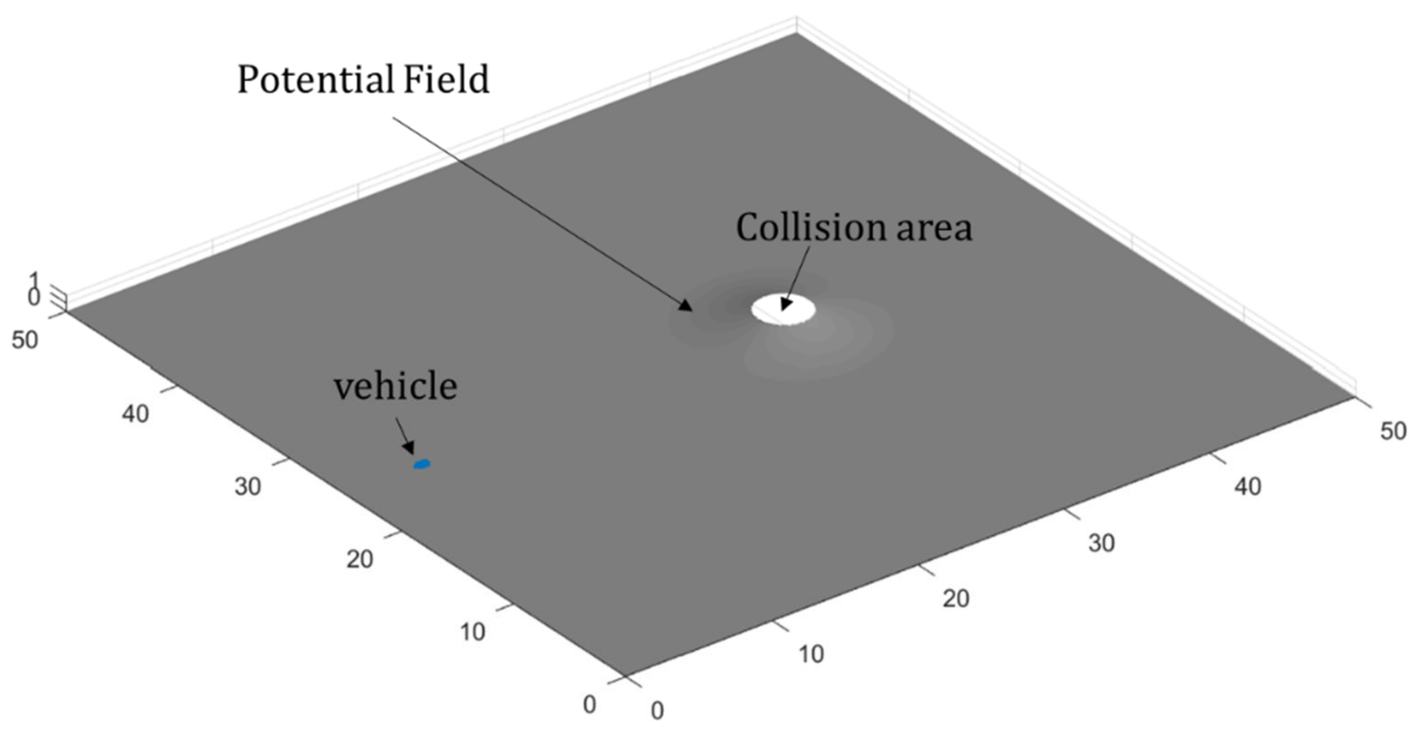
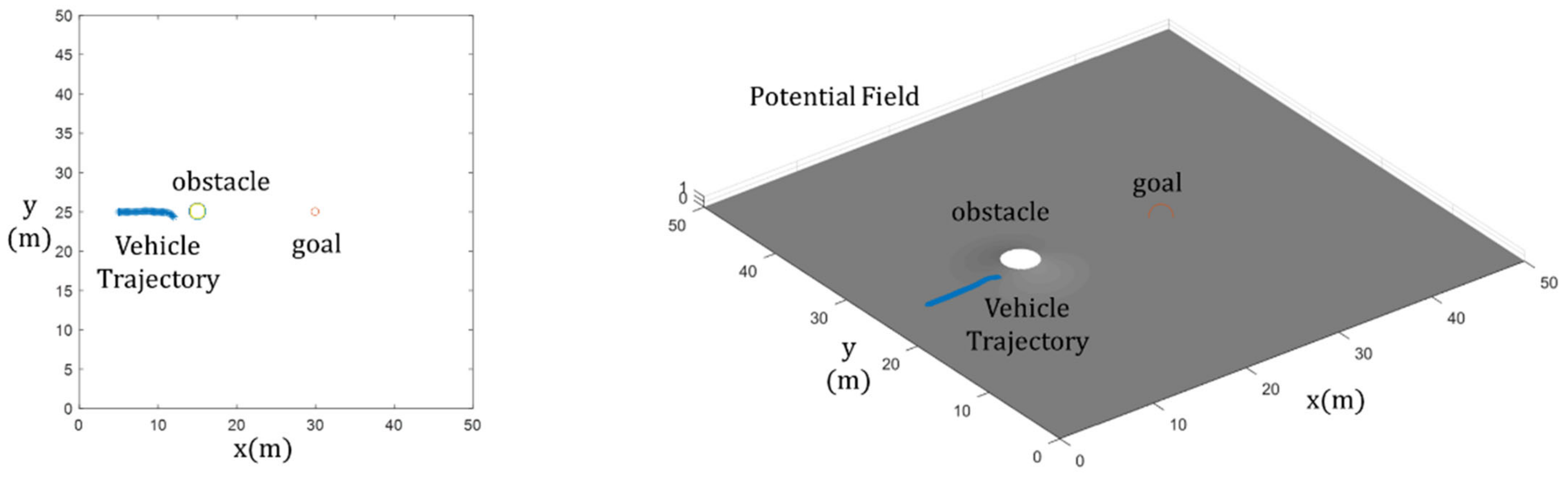
2.2. Potential Field
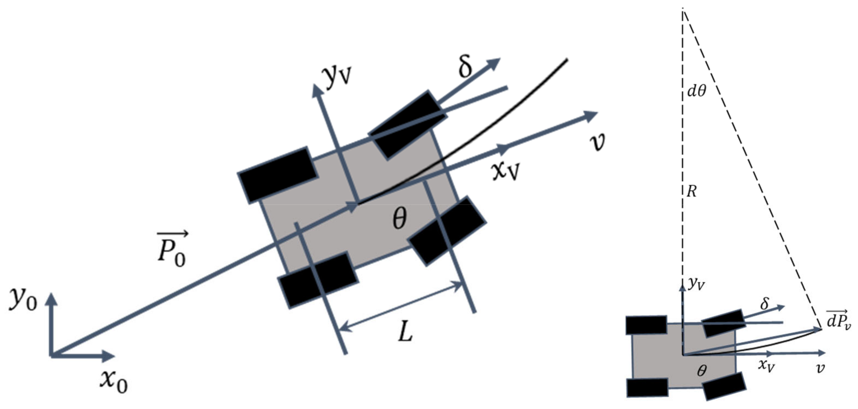
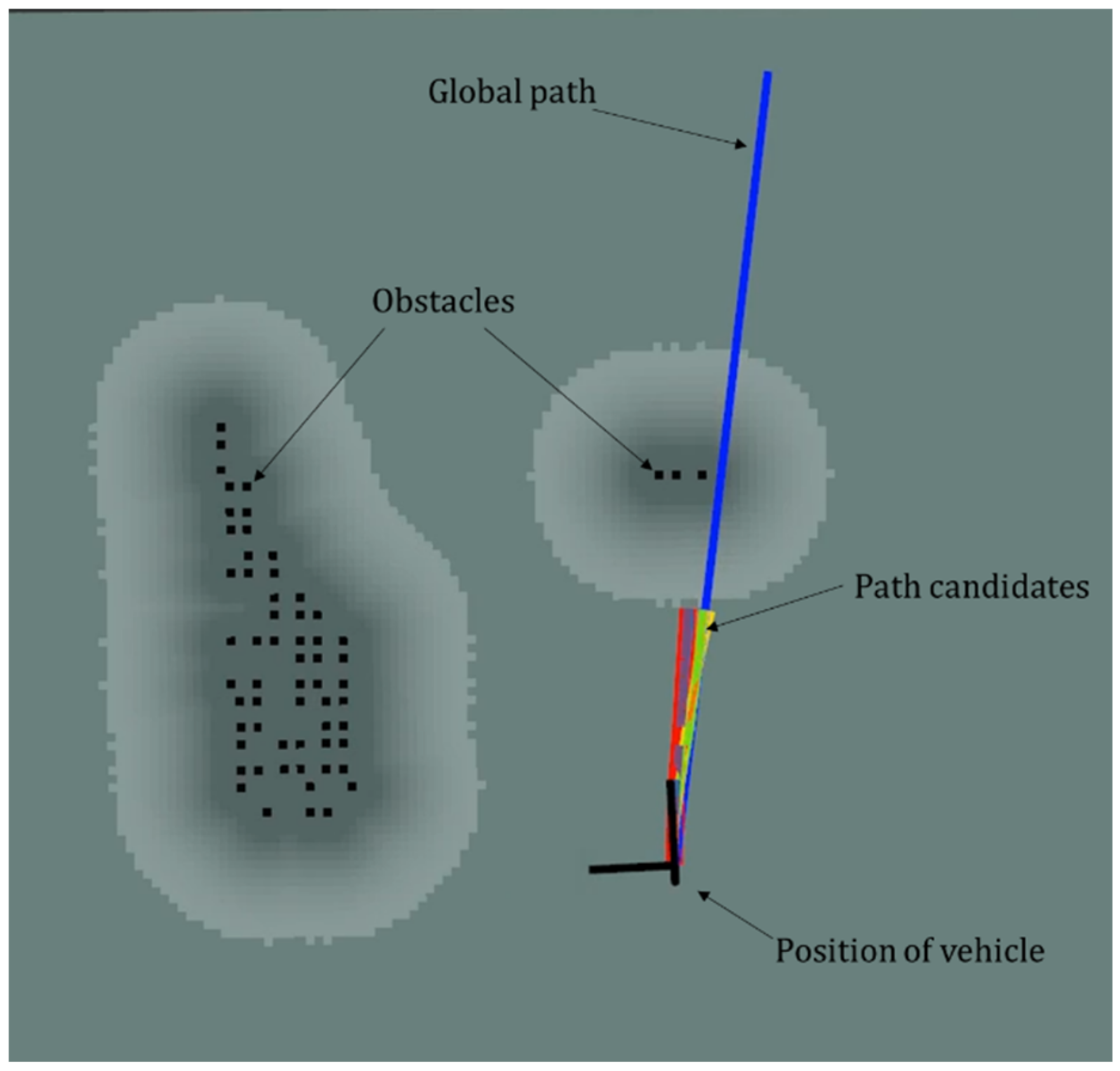
2.3. Model Predictive Path Planning
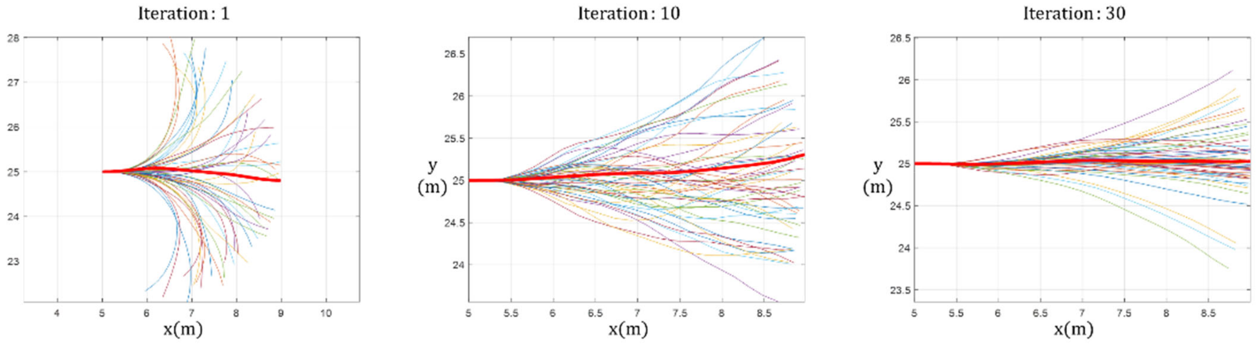
2.4. Particle Swarm Optimization
2.5. Cost Function for Selectiveness
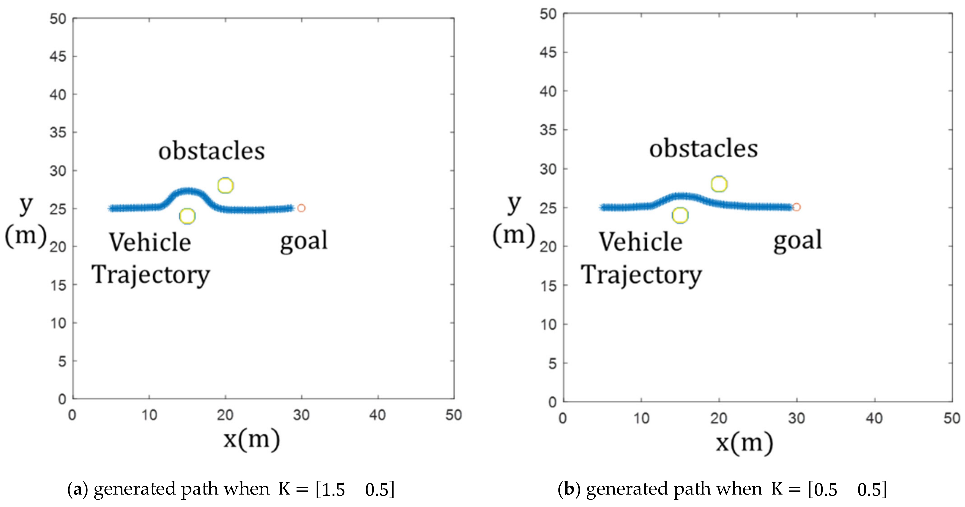
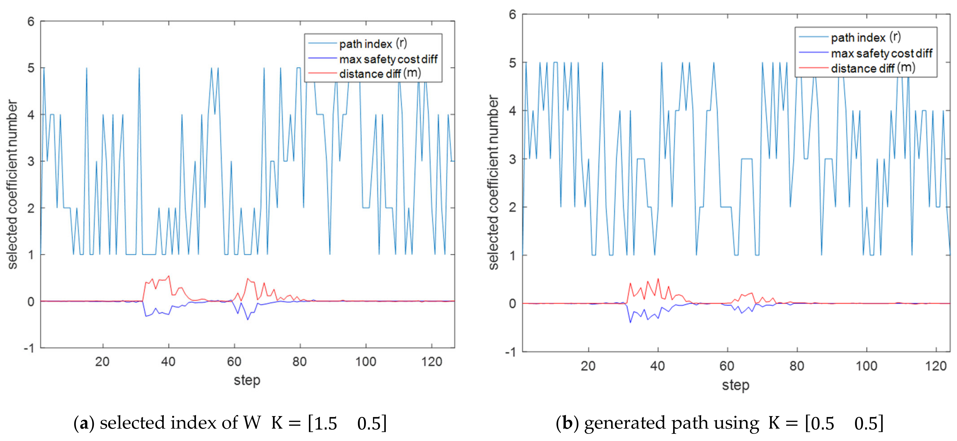
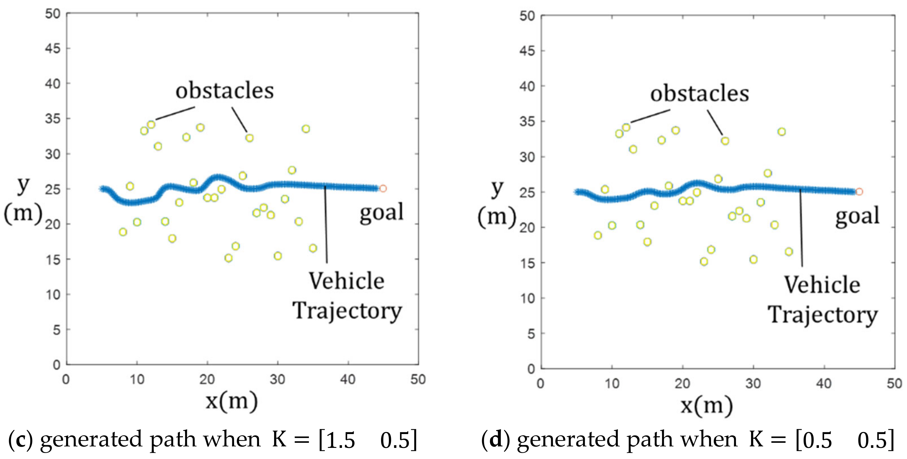
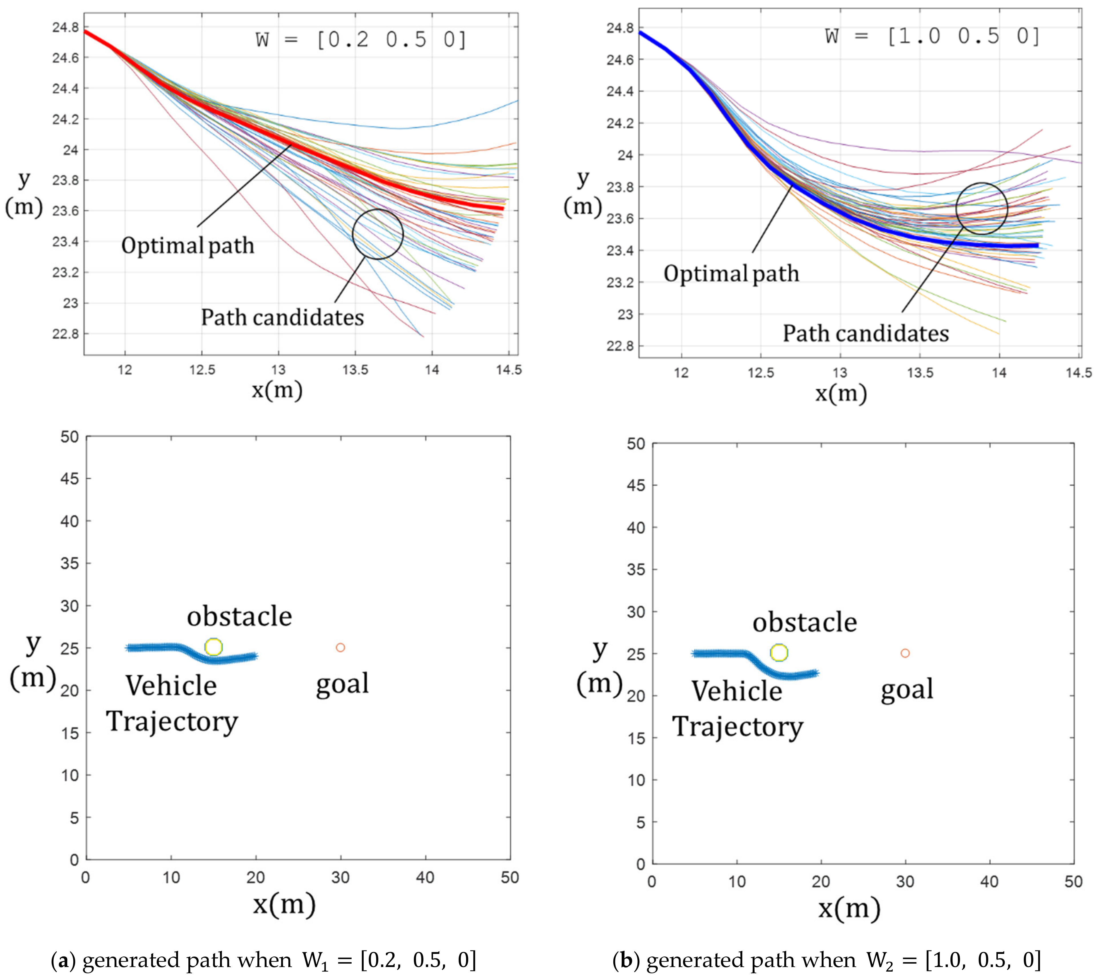
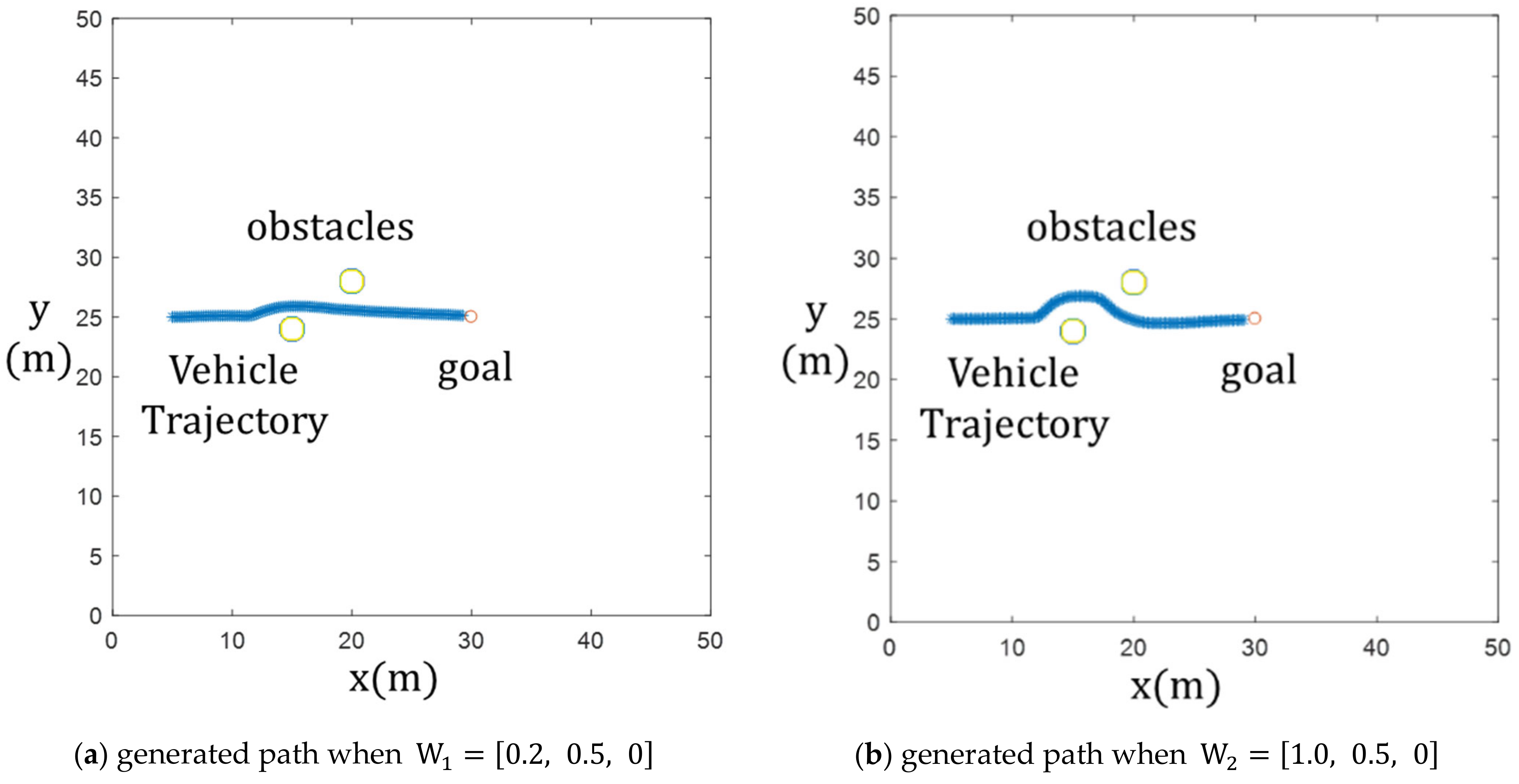
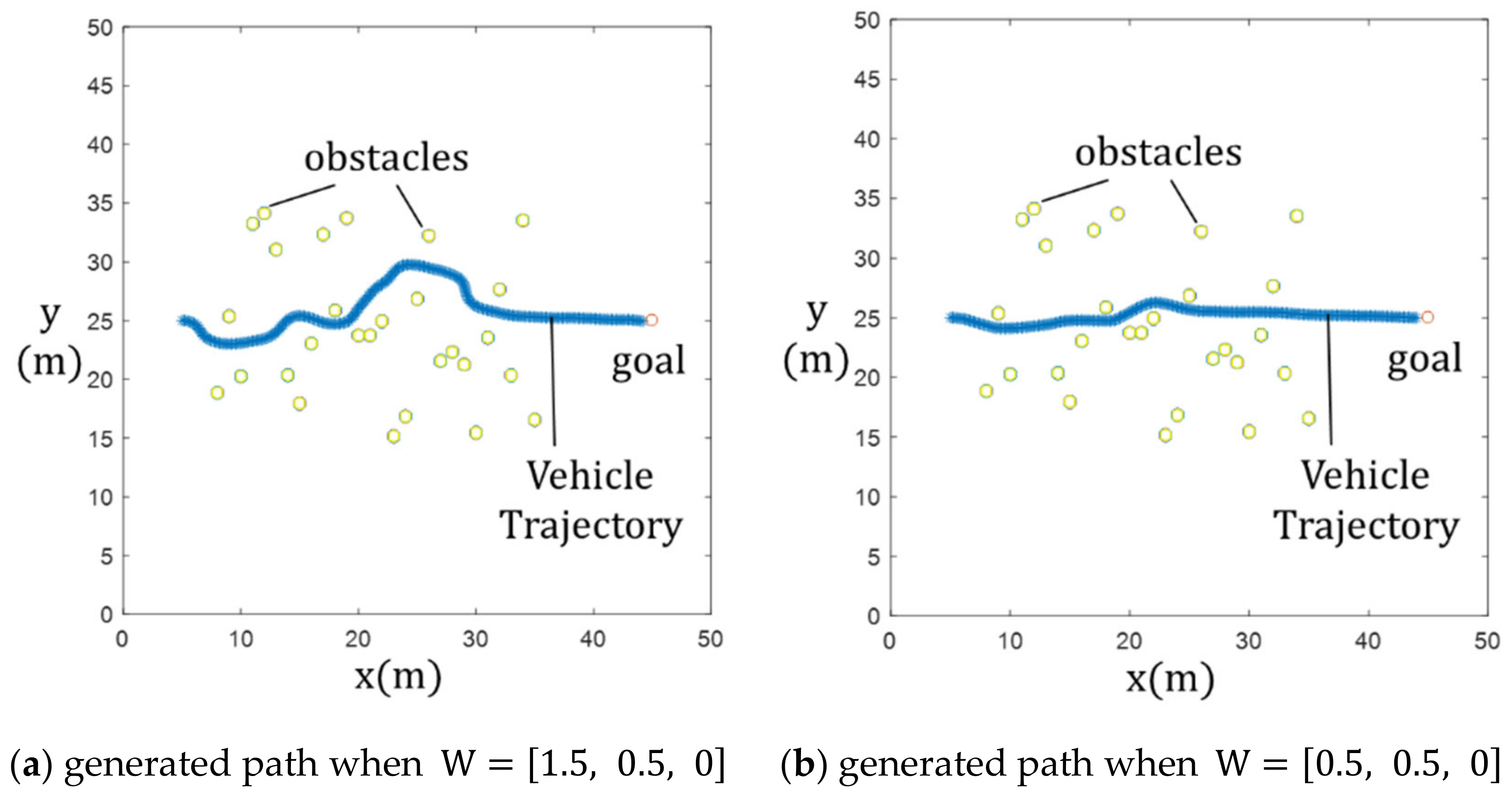
3. Simulation
| Algorithm 1: Pseudo code of the MPC-PF-PSO algorithm |
| initialize cost map using Potential Field as shown in Figure 2 costmap(x, y) = U(d) T—prediction time dt—time step N—Number of Particles M—Maximum number of iteration for all , = Max value = Max value initialize particles randomly for i = 1: N a random vector a random vector apply Equations (6)–(8) to calc Calc cost if if end for while j < M for i = 1: N apply Equations (11) and (12) to calc apply Equations (6)–(8) to calc Calc cost if if end for end while Calc cost end for Choose as a final path |
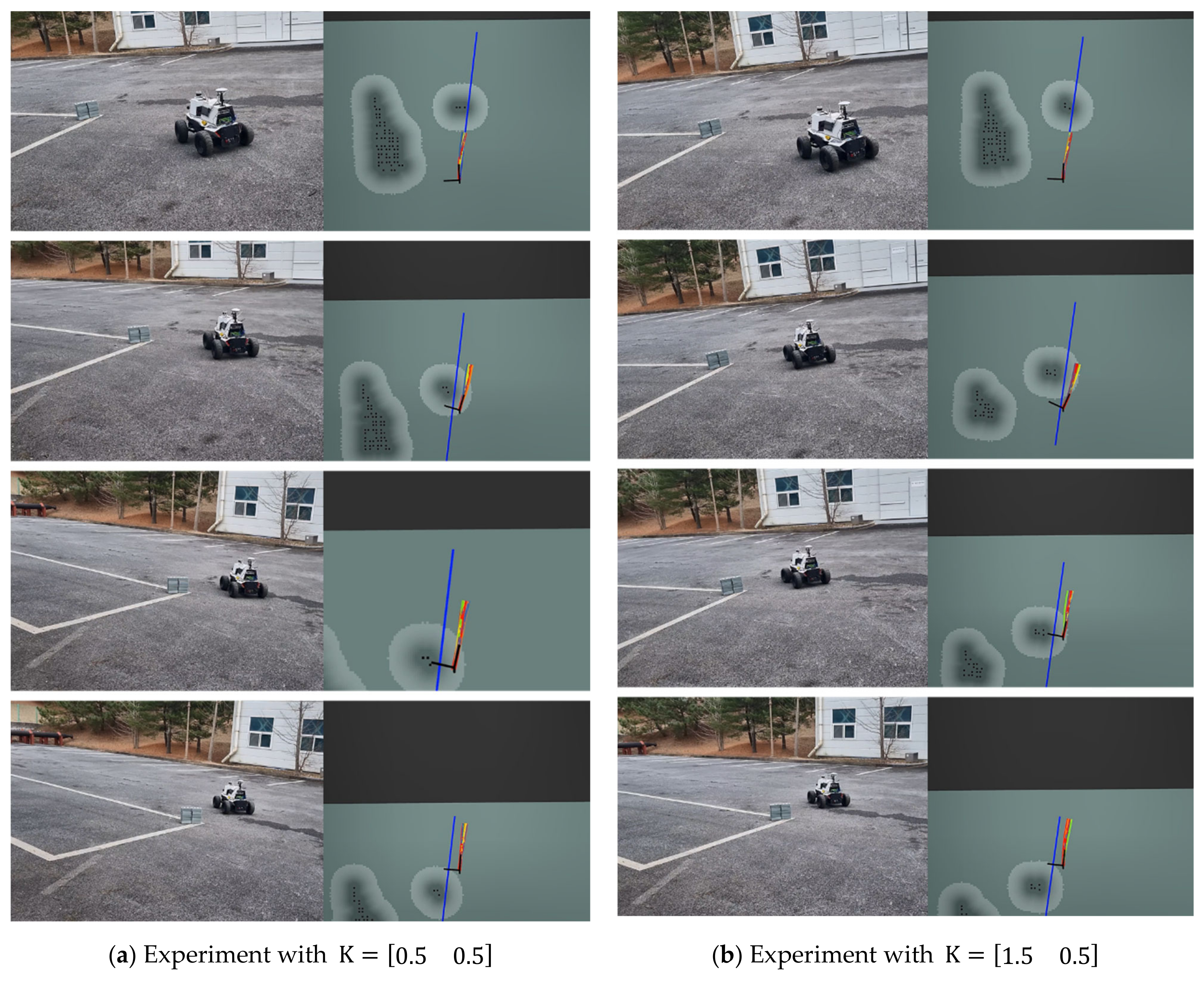
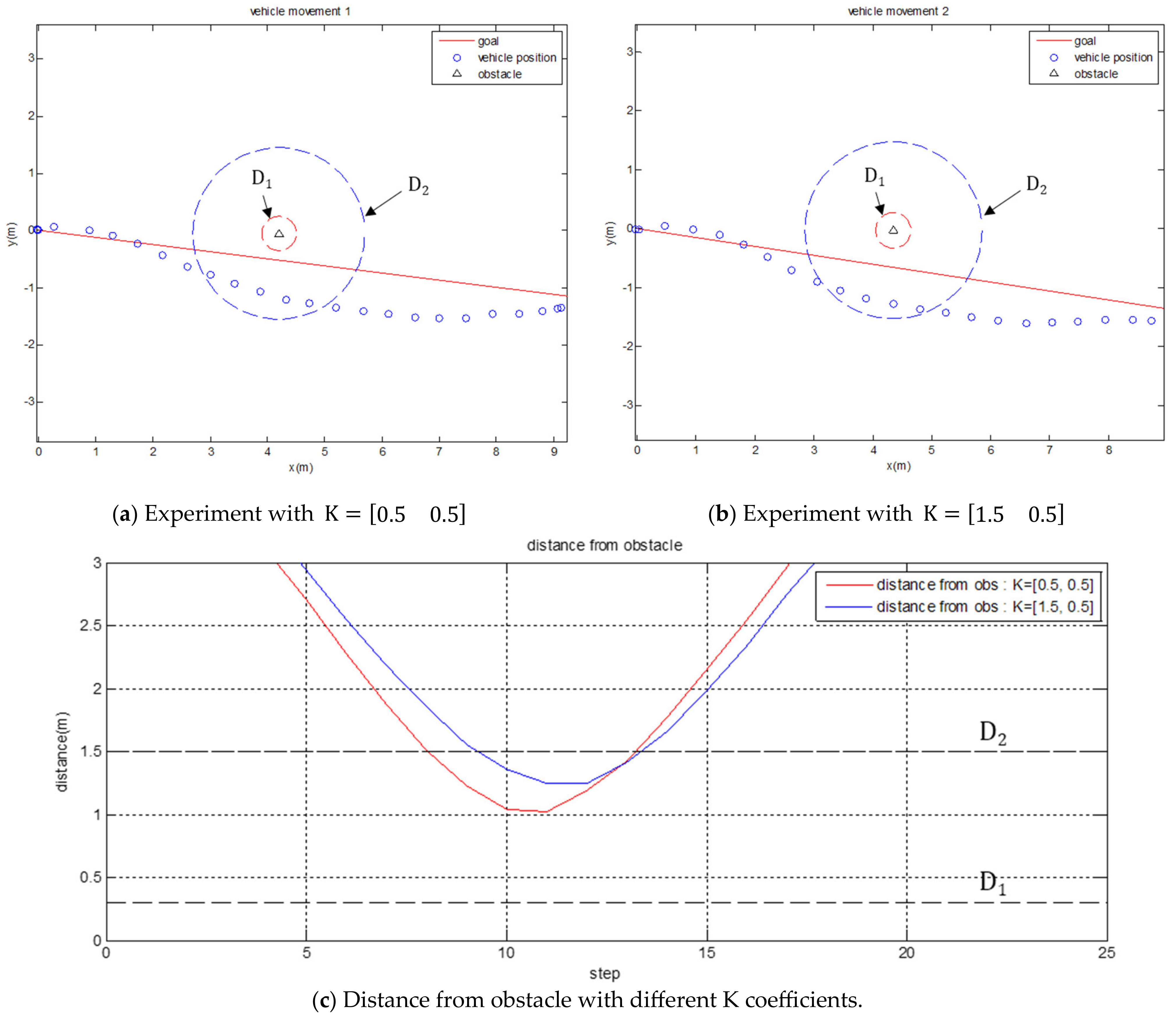
4. Experiment
5. Discussion
Author Contributions
Funding
Data Availability Statement
Conflicts of Interest
References
- González, D.; Pérez, J.; Milanés, V.; Nashashibi, F. A review of motion planning techniques for automated vehicles. IEEE Trans. Intell. Transp. Syst. 2015, 17, 1135–1145. [Google Scholar] [CrossRef]
- Lavalle, S.M. Planning Algorithms; Cambridge University Press: New York, NY, USA, 2006. [Google Scholar]
- Dijkstra, E.W. A note on two problems in connexion with graphs. Numer. Math. 1959, 1, 269–271. [Google Scholar] [CrossRef]
- Hart, P.E.; Nilsson, N.J.; Raphael, B. A formal basis for the heuristic determination of minimum cost paths. IEEE Trans. Syst. Sci. Cybern. 1968, 4, 100–107. [Google Scholar] [CrossRef]
- Elbanhawi, M.; Simic, M. Sampling-based robot motion planning: A review. IEEE Access 2014, 2, 56–77. [Google Scholar] [CrossRef]
- Kavraki, L.E.; Svestka, P.; Latombe, J.-C.; Overmars, M.H. Probabilistic roadmaps for path planning in high-dimensional configuration spaces. IEEE Trans. Robot. Autom. 1996, 12, 566–580. [Google Scholar] [CrossRef]
- LaValle, S.M.; Kuffner, J.J. Randomized kinodynamic planning. Int. J. Robot. Res. 2001, 20, 378–400. [Google Scholar] [CrossRef]
- Brezak, M.; Petrovic, I. Real-time approximation of clothoids with bounded error for path planning applications. IEEE Trans. Robot. 2014, 30, 507–515. [Google Scholar] [CrossRef]
- Koren, Y.; Borenstein, J. Potential field methods and their inherent limitations for mobile robot navigation. In Proceedings of the 1991 IEEE International Conference on Robotics and Automation, Sacramento, CA, USA, 9–11 April 1991. [Google Scholar]
- Kim, K. Predicted Potential Risk-Based Vehicle Motion Control of Automated Vehicles for Integrated Risk Management. Ph.D. Thesis, Seoul National University, Seoul, Republic of Korea, 2016. [Google Scholar]
- Kim, J.; Pae, D.; Lim, M. Obstacle Avoidance Path Planning based on Output Constrained Model Predictive Control. Int. J. Control Autom. Syst. 2019, 17, 2850–2861. [Google Scholar] [CrossRef]
- Mac, T.T.; Copot, C.; Tran, D.T.; De Keyser, R. Heuristic approaches in robot path planning: A survey. Robot. Auton. Syst. 2016, 86, 13–28. [Google Scholar] [CrossRef]
- Sfeir, J.; Saad, M.; Hassane, H.S. An improved artificial potential field approach to real-time mobile robot path planning in an unknown environment. In Proceedings of the 2011 IEEE International Symposium on Robotic and Sensors Environments (ROSE), Montreal, QC, Canada, 17–18 September 2011. [Google Scholar]
- Kim, D.H. Escaping route method for a trap situation in local path planning. Int. J. Control Autom. Syst. 2009, 7, 495–500. [Google Scholar] [CrossRef]
- Kim, D.H.; Shin, S. Local path planning using a new artificial potential function configuration and its analytical design guidelines. Adv. Robot. 2006, 20, 115–135. [Google Scholar] [CrossRef]
- Zuo, Z.; Yang, X.; Wang, Y.; Han, Q.; Wang, L.; Luo, X. MPC-based cooperative control strategy of path planning and trajectory tracking for intelligent vehicles. IEEE Trans. Intell. Veh. 2020, 6, 513–522. [Google Scholar] [CrossRef]
- Ji, J.; Khajepour, A.; Melek, W.W.; Huang, Y. Path planning and tracking for vehicle collision avoidance based on model predictive control with multiconstraints. IEEE Trans. Veh. Technol. 2016, 66, 952–964. [Google Scholar] [CrossRef]
- Huang, Z.; Wu, Q.; Ma, J.; Fan, S. An APF and MPC combined collaborative driving controller using vehicular communication technologies. Chaos Solitons Fractals 2016, 89, 232–242. [Google Scholar] [CrossRef]
- Du, X.; Htet, K.K.K.; Tan, K.K. Development of a genetic-algorithm-based nonlinear model predictive control scheme on velocity and steering of autonomous vehicles. IEEE Trans. Ind. Electron. 2016, 63, 6970–6977. [Google Scholar] [CrossRef]
- Van Heerden, K.; Fujimoto, Y.; Kawamura, A. A combination of particle swarm optimization and model predictive control on graphics hardware for real-time trajectory planning of the under-actuated nonlinear acrobot. In Proceedings of the 2014 IEEE 13th International Workshop on Advanced Motion Control (AMC), Yokohama, Japan, 14–16 March 2014. [Google Scholar]
- Thomas, J. Particle swarm optimization based model predictive control for constrained nonlinear systems. In Proceedings of the 2014 11th International Conference on Informatics in Control, Automation and Robotics (ICINCO), Vienna, Austria, 2–4 September 2014. [Google Scholar]
- Zuo, Z.; Dai, L.; Wang, Y.; Yang, X. Fast nonlinear model predictive control parallel design using QPSO and its applications on trajectory tracking of autonomous vehicles. In Proceedings of the 2018 13th World Congress on Intelligent Control and Automation (WCICA), Changsha, China, 4–8 July 2018. [Google Scholar]
- Khatib, O. Real-time obstacle avoidance for manipulators and mobile robots. Int. J. Robot. Res. 1986, 5, 90–98. [Google Scholar] [CrossRef]
- Kim, M.; Yoo, S.; Lee, D.; Lee, G. Local path-planning simulation and driving test of electric unmanned ground vehicles for cooperative mission with unmanned aerial vehicles. Appl. Sci. 2022, 12, 2326. [Google Scholar] [CrossRef]
- Choset, H. Robotic Motion Planning: Potential Functions; Robotics Institute, Carnegie Mellon University: Pittsburgh, PA, USA, 2010. [Google Scholar]
- Shin, J.; Kwak, D.; Kwak, K. Model predictive path planning for an autonomous ground vehicle in rough terrain. Int. J. Control Autom. Syst. 2021, 19, 2224–2237. [Google Scholar] [CrossRef]
- LI, X.; Wu, D.; He, J.; Bashir, M.; Liping, M. An improved method of particle swarm optimization for path planning of mobile robot. J. Control Sci. Eng. 2020, 2020, 3857894. [Google Scholar] [CrossRef]


| Variables | |
|---|---|
| Inertia of in PSO | |
| Weight of particle best in PSO | |
| Weight of global best in PSO | |
| Weight of safety in cost function | |
| Weight of distance from global path in cost function | |
| Weight of input in cost function |
Disclaimer/Publisher’s Note: The statements, opinions and data contained in all publications are solely those of the individual author(s) and contributor(s) and not of MDPI and/or the editor(s). MDPI and/or the editor(s) disclaim responsibility for any injury to people or property resulting from any ideas, methods, instructions or products referred to in the content. |
© 2024 by the authors. Licensee MDPI, Basel, Switzerland. This article is an open access article distributed under the terms and conditions of the Creative Commons Attribution (CC BY) license (https://creativecommons.org/licenses/by/4.0/).
Share and Cite
Kim, M.; Lee, M.; Kim, B.; Cha, M. Development of Local Path Planning Using Selective Model Predictive Control, Potential Fields, and Particle Swarm Optimization. Robotics 2024, 13, 46. https://doi.org/10.3390/robotics13030046
Kim M, Lee M, Kim B, Cha M. Development of Local Path Planning Using Selective Model Predictive Control, Potential Fields, and Particle Swarm Optimization. Robotics. 2024; 13(3):46. https://doi.org/10.3390/robotics13030046
Chicago/Turabian StyleKim, Mingeuk, Minyoung Lee, Byeongjin Kim, and Moohyun Cha. 2024. "Development of Local Path Planning Using Selective Model Predictive Control, Potential Fields, and Particle Swarm Optimization" Robotics 13, no. 3: 46. https://doi.org/10.3390/robotics13030046
APA StyleKim, M., Lee, M., Kim, B., & Cha, M. (2024). Development of Local Path Planning Using Selective Model Predictive Control, Potential Fields, and Particle Swarm Optimization. Robotics, 13(3), 46. https://doi.org/10.3390/robotics13030046