Abstract
This work presents the design and assessment of four control schemes for the monitoring and regulation of joint trajectories applied in the dynamic model of a SCORBOT-ER V plus robot, which includes the dynamics of the actuators, and the estimation of the friction forces present within the joints. The two classical control strategies calculated torque and PID, and the two advanced control strategies, fuzzy and predictive, are considered. In the latter case, a gravitational compensation stage is incorporated, as well as the inverse models of the motors and the transmissions of belt movement for each joint. Computational tests are performed by applying an external step-type disturbance to the third joint of the robot. Finally, an evaluation of the results obtained is presented through trajectory curves, joint errors, and the three performance indexes residual mean square, residual standard deviation, and index of agreement.
1. Introduction
Industrial robots have become the preferred automated tools for boosting production and decreasing expenses, largely due to two of their most vital capabilities: their ability to consistently execute repetitive physical tasks and their ability to accelerate procedures where meticulous accuracy is imperative.
In order for a manipulator robot to carry out a desired motion, it necessitates a controller capable of guiding the robot through the completion of the task. However, despite the central importance of manipulator control, it remains a domain filled with many practical and theoretical difficulties, stemming from the intricate dynamics governing these robots’ behavior, as well as the need for extremely precise trajectory planning when operating at high velocities under shifting loads [1].
As nonlinear, multivariable dynamic systems, manipulator robots pose substantial mathematical modeling challenges that complicate controller design and application. Exact representations demand precise link mass, inertia, and length data. Furthermore, practical uncertainties abound, from internal friction to external disturbances. Myriad control strategies attempt to handle such issues. Proportional-integral-derivative (PID) approaches prove hugely popular in industrial settings, owing to their conceptual simplicity and robustness across varying conditions. PID controllers successfully minimize manipulators’ steady-state errors, but remain sensitive to parametric and environmental uncertainty [2,3]. Alternative advanced methods may prove more resilient by accounting for robot dynamics and inevitable real-world variation. Still, PID’s virtues ensure widespread reliance, if almost always in conjunction with additional nonlinear controllers to fully stabilize performance.
Following classic PID, the Computed Torque Controller scheme (CTC) is the most used in the industry for the control of manipulator robots. Since the robot model is contained by the control law, CTC cancels the non-linearities of the robot’s dynamic model. This controller usually presents a better performance than PID, under the assumption that the dynamic parameters of the manipulator robot are known with relative accuracy [4,5]. Furthermore, CTC combines linear PD control and feedback dynamics, calculating it using real speed and the desired acceleration signals. This characteristic improves trajectory tracking and disturbance rejection. However, it presents two main shortcomings. Dynamic compensation is calculated based on a model with invariable dynamic parameters, i.e., the parameters vary during trajectory tracking, and uses linear PD with proportional and derivative constants to remove the tracking error [6,7].
As an expert system-based approach, fuzzy control has garnered substantial popularity by sidestepping the need to model certain systems with precise mathematical equations. Instead, it rapidly analyzes information using continuous truth values between “completely true” and “completely false”, yet still produces quick and accurate outputs. In this way, fuzzy control overcomes modeling complexity issues that can easily plague other techniques. Furthermore, fuzzy control is generally robust and tolerates inaccuracies and noise in the input data. Its logic programming is rule oriented. The order of these rules is arbitrary and allows for modifying both the type of membership functions and the number of rules [8,9]. Fuzzy logic lends itself well to controlling intricate processes that prove troublesome to model analytically. The challenges may stem from lacking comprehensive knowledge regarding the system’s mechanisms or stem from difficulties obtaining an accurate experimental identification [10]. Regardless of the root cause, fuzzy approaches can circumvent the need for precise models for processes that are too complex, nonlinear, or vague to characterize via conventional means.
The generic notion of model predictive control (MPC) was introduced through the petrochemical industry in the late 70s. From its beginnings, MPC has revolutionized control engineering, providing solutions to processes with complex dynamic behavior [11]. MPC also describes schemes that use a process model for two specific tasks: the explicit prediction of future behavior and the calculation of a corrective action for control, which are both required to direct the predicted output to values as close as possible to the desired objectives [12]. In essence, the predictive control technique employs an internal mathematical model and an optimization strategy to predict the system outputs within a time interval denominated prediction horizon. After determining a series of future control variables through optimization, MPC uses the error detected between the real output and the output predicted by the model to correct feedback. Therefore, it prevents the deviation of the controlled plant status from ideal values due the incompatibility of the model or environmental interference [13]. Operations close to the restrictions and the physical limitations of the actuators are among the main advantages of MPC. However, the formulation on which the algorithm is based implies high computational costs and, consequently, this strategy has to be implemented in computers that facilitate and support challenging matrix calculations [14,15].
This paper delineates the formulation, simulation, and performance analysis of four distinct control approaches to enable accurate multi-joint trajectory tracking for a 3-DoF (Degrees of Freedom) SCORBOT manipulator experiencing external perturbations. A classic PID scheme, a fuzzy logic controller that includes acceleration in its linguistic variables (differently from most methods), a torque control scheme that comprises of the inverse dynamic models of both actuators and transmission, and a predictive controller that incorporates gravity compensation are proposed.
2. Manipulator Kinematics and Dynamics: Foundational Models
The manipulator robot considered in this study corresponds to a SCORBOT-ER V plus. Three Degrees of Freedom, which allow for establishing its position in the (x,y,z) space, are employed in its design. Figure 1 shows a picture of the SCORBOT-ER V plus robot, together with its diagram.
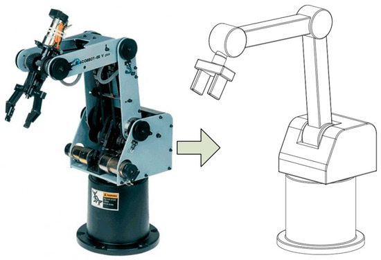
Figure 1.
SCORBOT-ER V plus robot and its diagram.
Figure 2 shows the diagram of the robot under study. To model its kinematics and dynamics, the coordinate axis and centroid systems consider q1, q2, q3 and l1, l2, l3 as generalized coordinates and lengths of the first, second, and third links, respectively. In turn, lc1, lc2, and lc3 represent the lengths of the first, second, and third links from origin to centroid.
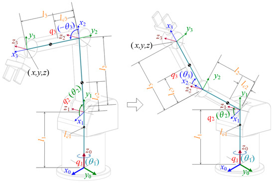
Figure 2.
Diagram of SCORBOT-ER V plus robot in two positions, considering the coordinate axis and centroid systems.
The kinematic model (direct and inverse) is obtained via applying the Denavit–Hartemberg and geometrical methods, respectively [16,17]. Using the cosine theorem, and considering the lengths of the three links, it is possible to calculate the angle . Then, from the angle and the spatial position (x,y,z), the angle can be obtained. The results are presented in Equations (1)–(4):
where: , , , , , and .
This kinematic model is required to establish the Cartesian trajectory of the robot’s end effector within its workspace. Based on the model, the desired joint path that each joint of the manipulator must follow can be determined.
The dynamics governing the manipulator behavior derive from Lagrange’s seminal formulation, which elegantly extends Euler’s foundational work using the energy-based Equation (5) [18]. This powerful approach yields rich dynamic models by exploiting deep connections between system kinetics and kinematics.
In the above dynamic formulation, τ denotes the (n × 1) generalized force vector, M refers to the (n × n) inertia matrix, C constitutes an (n × 1) vector of centrifugal and Coriolis forces, q represents joint position coordinates, stands for corresponding joint velocity terms, G signifies the (n × 1) gravitational force vector, refers to joint accelerations as an (n × 1) vector, F encapsulates frictional forces in an (n × 1) format, and n corresponds to the number of Degrees of Freedom.
For a mechanical structure composed of links coupled through rotational joints to move and incorporate the position of its end effector to a determined joint trajectory, the inertial forces present in each link due to acceleration needs to be overcome. The physical interaction between the rotational links also requires compensation for centrifugal and Coriolis forces. To vertically position the centers of mass of each coupled link, the gravitational action, both upward and downward, has to be overcome, depending on the direction of the movement. Furthermore, the resistance forces that act in a direction opposite to the direction of movement of each link of the mechanical structure (static and dynamic friction) need compensation. Due to the characteristics of this behavior, torques should be applied in each joint via actuators in order to compensate these forces, as indicated in Equation (5).
The derived dynamic model motion equations governing the manipulator’s behavior are detailed in the Appendix A under Dynamic Model. This dynamic model is necessary to link forces and torques, which are required to be applied in each joint, with the actuation elements and the movement of the robot. The actuation elements correspond to PITTMAN brand DC motors and GM9413A models for the first three joints [19,20,21].
This information allows for conducting simulations of the robot’s movement to design and test the controllers that are discussed in the next section. In this way, the necessary assessments and corrections will be carried out to obtain the best control algorithm performance.
The values of the parameters considered for the manipulator robot are shown in Table 1 [16].

Table 1.
Manipulator Specifications.
3. Controller Designs
3.1. Computed Torque Controller
The algorithm consists of the application of a torque to compensate the centrifugal and Coriolis effects, as well as the gravitational and friction effects, as indicated in (6) [22,23].
where is the estimation of the inertia matrix (n × n), is the estimation of the centrifugal and Coriolis force vector (n × 1), is the estimation of the gravitational force vector (n × 1), is the estimation of the friction force vector (n × 1), is the joint desired acceleration vector (n × 1), is a definite positive diagonal matrix (n × n), and is a definite positive diagonal matrix (n × n). Finally, in terms of the joint coordinates of the manipulator robot, corresponds to the position error vector and to the speed error vector. To make the terms in Equations (5) and (6) equal, we can use the following equation:
Since is a definite positive matrix that consequently can be inverted, Equation (7) is reduced to Equation (8):
The proposed method for the computed torque controller, besides the revised control law, includes the dynamic model of the robot actuators (direct current motors) together with the movement transmission ratio (belt). This has the objective of simulating a system much closer to the real one. The diagram of its design is observed in Figure 3.
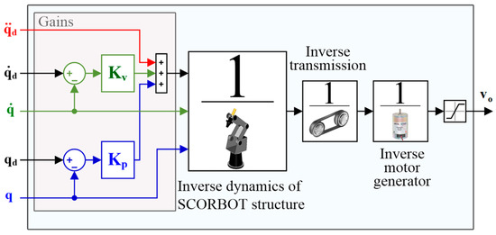
Figure 3.
Diagram of the designed calculated torque controller.
The and gains incorporated within the control law are enumerated in Table 2.
Table 2.
Gains of the computed torque controller.
3.2. Predictive Controller
Predictive control is based on a weighted sum of squared errors and control efforts. At any time instant , an optimal control problem is solved for a finite and future N horizon, where a function is minimized. Such a function has restrictions, as indicated in (9), and quantifies the difference between the plant output () and the reference (r), as well as the control effort (u) [13,24].
In general, within the considered horizon, the future output is expected to follow a specific reference signal while penalizing the control effort required for this task. The general equation of such an objective function has the shape indicated in (10):
where is the optimal prediction or future output that is steps forward from the process output (with known data until instant ), and is the future reference trajectory. and define the prediction horizon. The variation of the control action corresponds to the control effort. The control horizon is , while , are weighting sequences or weights. In the objective function, and specifically represent the relative weights of the importance of each component of the error in the output and control effort, respectively. Usually, these parameters do not vary with time and are thus considered constant values.
As observed in Figure 4, a predictive controller based on the model was, which incorporated gravity compensation (MPC + G) for each designed joint, in order to reduce the effect of the external disturbance.
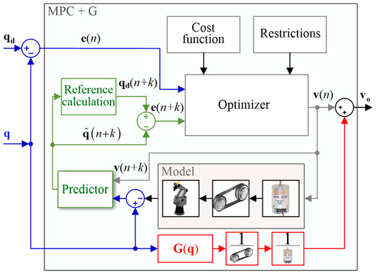
Figure 4.
Diagram of the structure of the predictive controller with gravity compensation.
Table 3 indicates the values of the parameters used for the tuning of the predictive controllers with gravity control. These parameters were the sampling time, prediction horizon, and control horizon. This compensation accounts for more than simply the manipulator’s gravitational forces G by further incorporating the inverse dynamics of both the actuators and transmission system. These models were obtained via the training of neural networks with inverse modeling.
Table 3.
Gains of the predictive controller.
3.3. Fuzzy Logic Controller
As an expert system methodology, fuzzy control uniquely enables handling complex dynamic systems without reliance on precise mathematical models. Instead, as depicted in the generic schema in Figure 5, fuzzy controllers employ linguistic variables and rule-based inferences to map the inputs to the desired outputs. This grants fuzzy approaches great flexibility in tackling control challenges that lack analytical system representations or that have vague, qualitative dynamics.
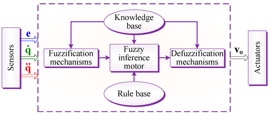
Figure 5.
Modular formulation of a fuzzy logic controller.
Broadly speaking, fuzzy control algorithms derive their outputs from joint positional details and velocity measurements furnished by proprioceptive sensors like encoders or tachometers which are situated on the manipulator links [25,26]. Several research efforts integrate fuzzy techniques for processing positions and velocity sensor data, including hybrid force/motion and force/position schemes, fuzzy PID approaches, obstacle-avoidant adaptive designs, fractional-order fuzzy control, and PID-guided adaptive laws for highly linear industrial processes facing substantial parameter fluctuations, noise, and instability [27,28]. This work, unlike the examples above, deals with the design and simulation of three fuzzy controllers—one per robot joint—that include the second derivative of the joint position as one of its linguistic variables. As shown in Figure 6, each controller has three inputs: error, speed, and position acceleration. Its output is the voltage entering the actuators of each joint.
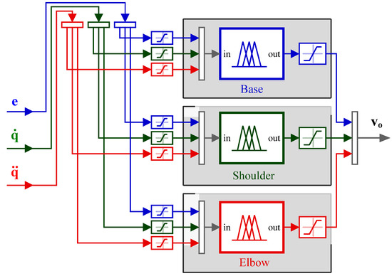
Figure 6.
Diagram of the fuzzy controller designed.
Table 4 enumerates the specific linguistic variables underlying each controller, detailing the universes of discourse (U) and membership function terms (T). All implementations utilize the classical Mamdani inference methodology.
Table 4.
Gains of the predictive controller.
The terms NB, NS, Z, PS, and PB correspond to Negative Big, Negative Small, Zero, Positive Small, and Positive Big, respectively. Likewise, LVF, LF, S, RF, and RVF represent Left Very Fast, Left Fast, Slow, Right Fast, and Right Very Fast; N, Z, and P correspond to Negative, Zero, and Positive, and LB, LS, Z, RS, and RB correspond to Left Big, Left Small, Zero, Right Small, and Right Big, respectively.
The rule base of each controller is a combination of the terms defined, which uses sentences with the structure if … else, together with the logical operator and.
3.4. PID Controller with Anti-Windup
The first control scheme implemented for the manipulator is an anti-windup PID approach, independently tuned for each joint using iterative empirical parameter adjustments to balance trajectory accuracy and rapidity. The controller diagram in Figure 7 displays the overflow prevention structure that improves performance by negating the integrator windup in the event of control saturation [29,30,31].
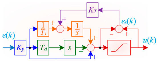
Figure 7.
Block diagram of PID controller with anti-windup.
The PID controller’s discrete-time step output u(k) is formulized according to (11) as follows:
The variables in (11) consist of the proportional gain ; the integral time constant ; the derivative time constant ; the sampling period ; the integral gain ; the position error e as the difference between setpoint and observed values; and the saturated error es, defined as the discrepancy between clipped and raw controller error signals. The parameterized constants underlying the implemented anti-windup PID appear in Table 5.
Table 5.
Gains of the PID controller.
4. Results
In this section, the results of each control strategy are shown. With this purpose, a desired Cartesian trajectory is defined within the workspace of the robot, as indicated in Figure 8. Through inverse kinematics, qd the desired joint trajectory—composed of qdn with n = 1, 2, 3—is obtained considering a total duration of 24 s, as shown in Figure 9.
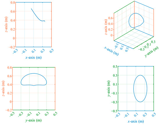
Figure 8.
Desired Cartesian trajectory.
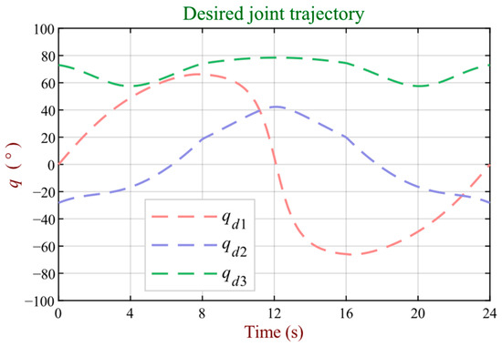
Figure 9.
Desired joint trajectory.
The manipulator attempts to track the reference joint trajectory under each control approach, enabling comparative assessment based on quantified performance metrics, specifically residual mean square (RMS), residual standard deviation (RSD) and the index of agreement (IA) coefficient [32].
4.1. Results with External Disturbance
Trajectory tracking and regulation results for the computed torque, predictive with gravity compensation, and the fuzzy and PID control are presented in Figure 10, Figure 11, Figure 12 and Figure 13. The external disturbance of the tests consists of a 2 N·m torque step that is applied to joint 3 (elbow) thirteen seconds after the robot starts moving. In each figure, the simulated joint trajectory is expressed by q (composed of qn, with n = 1, 2, 3).
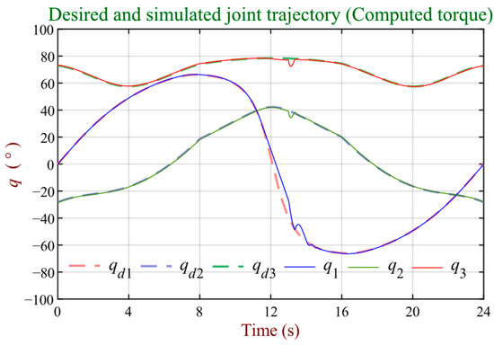
Figure 10.
Comparison of desired and simulated joint trajectories when using computed torque.
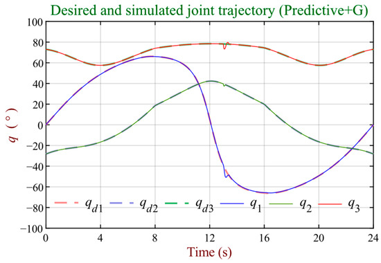
Figure 11.
Comparison of desired and simulated joint trajectories when using the predictive controller.
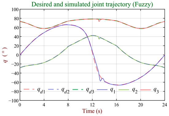
Figure 12.
Comparison of desired and simulated joint trajectories when using the fuzzy controller.
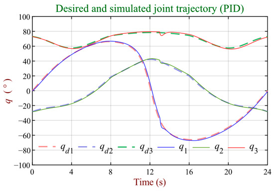
Figure 13.
Comparison of desired and simulated joint trajectories when using the PID controller with anti-windup.
4.2. Joint Error Results
To determine the performance indexes for each controller and Degree of Freedom, the joint error curves are presented according to algorithm, i.e., computed torque, predictive with gravity compensation, and the fuzzy and PID control, from Figure 14, Figure 15, Figure 16 and Figure 17. In each figure, the resulting joint error e (composed of en, with n = 1, 2, 3.) is calculated as the difference between the desired joint trajectory qd and the resulting simulated trajectory q.
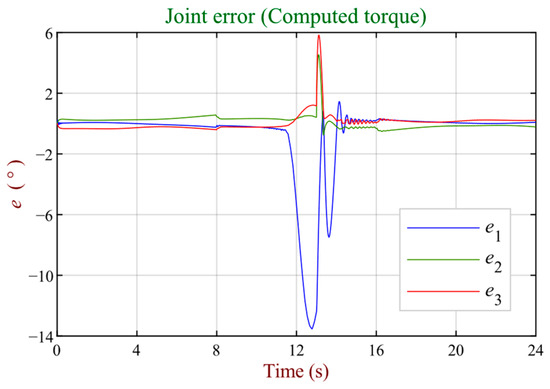
Figure 14.
Joint trajectory error when using the computed torque controller.
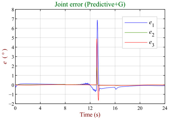
Figure 15.
Joint trajectory error when using the predictive controller with gravity compensation.
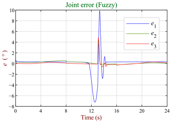
Figure 16.
Joint trajectory error when using the fuzzy controller.
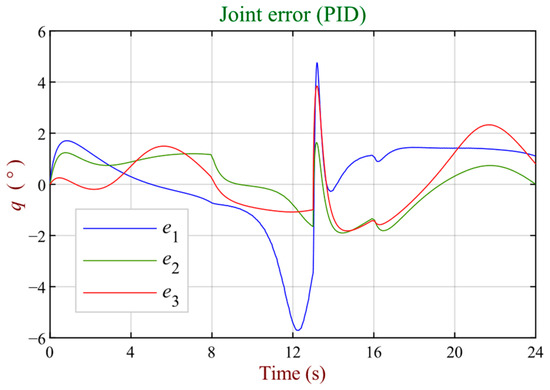
Figure 17.
Joint trajectory error when using the PID controller with anti-windup.
4.3. Performance Indexes
The indexes considered to assess the performance of the controllers correspond to an RMS, RSD, and IA, which are mathematically expressed Equations (12)–(14), respectively [32].
where n corresponds to the total number of observations, denotes the observed values, and indicates the predicted values. Additionally, , and , where is the mean value of the observations.
The performance metrics quantified for each control scheme include RMS, RSD, and IA, graphed per joint in Figure 18, Figure 19 and Figure 20 across the single, dual, and triple joint configurations incorporating the base, shoulder, and elbow (1, 2, and 3).
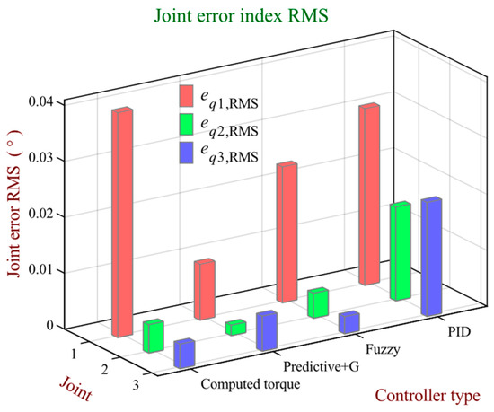
Figure 18.
Comparison chart for joint error index RMS.
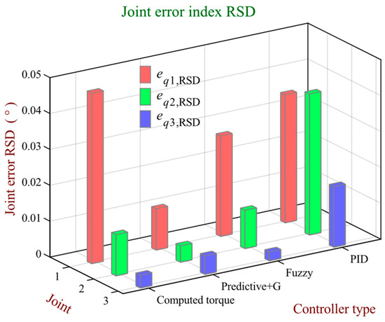
Figure 19.
Comparison chart for joint error index of RSD.
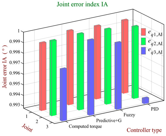
Figure 20.
Comparison chart for joint error of IA.
According to the results obtained, it is observed that, although the test disturbance was applied only to joint 3, the greatest errors occur in joint 1 in terms of regulation, which corresponds to the rotational base of the robot. This rotational base is not affected by gravitational effects, and therefore such results seem contradictory. However, approximately at 10–14 s of the trajectory, the largest slope is detected at joint 1. This means that the effects of the test disturbance are added to the torque limitations of the joint 1 actuator, according to the requirement of excessive speed in the indicated section.
However, in the predictive controller, more gravity compensation presents the least joint peak deviation, as indicated in Figure 11 and Figure 15. In this context, the calculated torque controller shows considerable difficulty in facing the demands of speed and torque limitations, in addition to the test disturbance, as shown in Figure 10.
It should be noted that, in the first design stage, the predictive controller without gravity compensation was considered. However, its performance to compensate for the effects of the test disturbance was not satisfactory, particularly for joints 2 and 3. Thus, it was decided to incorporate a gravitational compensation section based directly on Equations (24) and (25). The result was again not satisfactory, as the fact that this compensation was applied directly as a voltage supply signal to the actuators resulted in it being very aggressive. Therefore, it was decided to reduce gravitational compensation through the inverse models of the belt motion transmissions and the PITTMAN motors, as shown in Figure 4. In the latter case, the models were obtained through the training of artificial neural networks by an inverse model. However, an important limitation regarding the predictive controller with gravity compensation, unlike the other controllers analyzed, refers to the fact that it presented a higher computational cost in terms of the execution times of the simulations. This disadvantage can be explained by the iteration requirements to solve an optimization problem [13]. Such a characteristic can be decisive when making a real practical implementation without having high-performance processors.
In terms of tracking (before the application of the test disturbance), the resulting joint trajectories that more closely approximate the desired joint trajectory correspond to those provided by the predictive with gravity compensation and diffuse controllers, as seen in Figure 11 and Figure 12, respectively. Regarding the performance of the PID controllers and calculated torque, the latter presents higher tracking accuracy than PID and notably lower joint errors, as shown in Figure 14 and Figure 17. This result relates to the precise knowledge of the dynamic parameters that characterize the robot [5]. However, since these results are obtained through computational simulations, similar results cannot be ensured in a real practical implementation.
When analyzing joint 1, the predictive controller with gravity compensation yielded the smallest RMS and RDS errors, as well as an IA value closest to 1. These values were 0.0010, 0.0115, and 0.9998, respectively. In turn, for the same joint, the computed torque controller presents the highest RMS and RDS errors, as well as the IA value farthest from 1. Such values are 0.0402, 0.0475, and 0.9992, respectively.
Regarding joint 2, the predictive controller with gravity compensation exhibits an excellent performance, characterized by an RMS error equal to 0.0019, an RDS value of 0.0046, and an IA index of 1.0000. Conversely, it must be noted that the highest RMS and RDS errors, together with the IA value farthest from 1, correspond to the PID controller, whose respective values for the three indexes are 0.0168, 0.0393, and 0.9996.
According to the tracking and regulation results of joint 3, the fuzzy controller exhibits the lowest RMS (0.0031) and RSD (0.0025) errors. However, the IA value closest to 1 is presented by the predictive controller with gravity compensation, which has a 0.9999 value. In this context, the PID controller shows the lowest performance, with values for the RMS, RSD, and IA indexes being equal to 0.0204, 0.0169, and 0.9933, respectively.
Table 6 aggregates the RMS, RSD, and IA metrics quantified per controller for the single, dual, and three joint configurations encompassing the base, shoulder, and elbow manipulator links.
Table 6.
Performance indexes.
Optimally, RMS and RSD values approach 0, indicating negligible tracking errors, while the IA nears 1, conveying a high correlation between the reference and measured joint trajectories.
In general terms, according to the calculated performance indices, the performances of the Fuzzy, Predictive + G, and Computed Torque controllers are similar. However, when analyzing the performance in terms of the disturbance rejection, it is possible to highlight that the Predictive + G controller takes considerably less time (than the other controllers) to compensate for the disturbance projected on the base and shoulder of the robot, with times of 0.45 and 0.14 s, respectively. On the other hand, the disturbance compensation time at the robot’s elbow is approximately similar for the three aforementioned controllers. This can be explained by the fact that the disturbance was applied directly to the robot’s elbow, and the correction speed is conditioned by the torque limitations of the PITTMAN actuators. The presented results were obtained through the use of various tests, including making modifications to the parameters of each controller until the best possible result for each of them was obtained. In this way, it is possible to affirm that the performance of the controllers must depend on the tuning parameters. Table 7 shows the disturbance compensation times.
Table 7.
Disturbance compensation times.
5. Conclusions
This work dealt with the design and assessment of four joint controllers, namely computed torque, predictive with gravity compensation, fuzzy, and PID controllers. Such control strategies are applied to the dynamic model of a SCORBOT-ER V plus robot for trajectory tracking and regulation. The robot was subject to an external disturbance on its elbow, which is consistent with a 2 N·m torque step, thirteen minutes after the robot started moving.
The manipulator’s nonlinear dynamics derive from a Euler–Lagrange formulation, harnessing energy balancing to the encapsulate actuator kinetics and friction phenomena innate to joint articulation, yielding a rich representation.
A series of control algorithm simulations were conducted through a complete simulation environment created with the tools of the MatLab/Simulink software R2022A, developed by MathWorks, Portola Valley, CA, United States.
Comparative control assessment employed three metrics to quantify the trajectory tracking accuracy—RMS, RSD, and IA coefficient—with superior performances exhibiting diminishing error-based indices and unity agreement.
The parameters of each controller were successively empirically adjusted until the best results were obtained; these results were presented in this work. A particular case corresponds to the predictive controller, since it was not able to correct the errors in joints 2 and 3, which were affected by the gravitational force. In this case, the tracking and regulation response is achieved with joint errors close to zero by incorporating a gravitational compensation, weighted by the inverse models of the motors and the motion transmission belts of each joint. However, a higher computational cost was also observed in terms of the execution times of the simulations, unlike with the other controllers analyzed. This disadvantage can be decisive when making a real practical implementation without having high-performance processors.
The controllers that presented the lowest computational cost were the PID controllers and the calculated torque. The latter had a tracking accuracy superior to that of PID. However, it should be noted that these results were obtained via computer simulations. In this way, a similar performance cannot be ensured in a real implementation if the precise dynamic parameters that characterize the robot are not available.
Broadly, the designed and assessed controllers demonstrate adequate setpoint tracking, with near-zero residuals and a unity agreement indicating excellent reference trajectory reproduction. However, after a meticulous analysis that considers the external disturbance, the predictive control scheme with gravity compensation achieved a higher accuracy in the tracking and regulation of the SCORBOT robot joint trajectory.
In particular, the predictive controller with gravity compensation exhibited an IA equal to 1 in the case of joint 2. In this same scenario, the highest error was found in the computed torque and PID controllers. Furthermore, the performance of the fuzzy controller obtained the lowest tracking and regulation errors in joint 3.
6. Future Work and Limitations
One of the main limitations of this work is that results have only been obtained at the level of computational simulations. In turn, the predictive controller has a high computational cost when solving an optimization problem. This requirement could become more demanding if a gravitational compensation stage, along with the inverse models of the belt drives and motors for each joint, is implemented, especially if the inverse models are generated through artificial neural networks using an inverse model.
Future efforts will advance manipulator control research through continued analysis and novel methodology development. This stage comprises the real practical implementation of such algorithms in real industrial robots to compare the real practical results with those of computer simulations. In addition, the search for training mechanisms is also considered, which would allow for reducing the dependence on parameter accuracy required by the calculated torque controller, mainly when a real practical implementation needs to be conducted.
Author Contributions
Conceptualization, J.K. and C.U.; Methodology, J.K. and C.U.; Software, J.K. and C.U.; Validation, J.K. and C.U.; Formal analysis, J.K. and C.U.; Investigation, J.K. and C.U.; Resources, J.K., C.U. and R.A.; Data curation, J.K., C.U., H.V. and C.B.; Writing—original draft preparation, J.K. and C.U.; Writing—review and editing, J.K. and C.U.; Visualization, J.K., C.U., H.V. and C.B.; Supervision, J.K. and C.U.; Project administration, J.K., C.U. and H.V.; Funding acquisition, J.K., C.U. and R.A. All authors have read and agreed to the published version of the manuscript.
Funding
This research received no funding.
Institutional Review Board Statement
Not applicable.
Data Availability Statement
All date are contained within this article.
Acknowledgments
This work was supported by the Faculty of Engineering of the University of Santiago of Chile, Chile.
Conflicts of Interest
The authors declare no conflict of interest.
Appendix A. Dynamic Model
The dynamic model of the manipulator robot is obtained using the Euler–Lagrange formulation [18]. From Equation (5), the dynamic model can be expressed through Equations (A1–(A2) [17]:
where c2·2 = cos(2θ2); s2·2 = sin(2θ2); m1, m2, and m3, represent the mass of the first, second, and third links, respectively. In turn, l1zz, l2zz, and l3zz indicate the inertia moments of the first, second, and third links with respect to the first z axis of their respective joints.
References
- Chen, D.; Zhang, Y.; Li, S. Tracking Control of Robot Manipulators with Unknown Models: A Jacobian-Matrix-Adaption Method. IEEE Trans. Ind. Inform. 2018, 14, 3044–3053. [Google Scholar] [CrossRef]
- Hernández-Guzmán, V.M.; Orrante-Sakanassi, J. Global PID Control of Robot Manipulators Equipped with PMSMs. Asian J. Control 2018, 20, 236–249. [Google Scholar] [CrossRef]
- Urrea, C.; Saa, D. Design, Design, Simulation, Implementation, and Comparison of Advanced Control Strategies Applied to a 6-DoF Planar Robot. Symmetry 2023, 15, 1070. [Google Scholar] [CrossRef]
- Chen, C.; Zhang, C.; Hu, T.; Ni, H.; Luo, W. Model-assisted extended state observer-based computed torque control for trajectory tracking of uncertain robotic manipulator systems. Int. J. Adv. Robot. Syst. 2018, 15, 1729881418801738. [Google Scholar] [CrossRef]
- Chaturvedi, N.K.; Prasad, L.B. A Comparison of Computed Torque Control and Sliding Mode Control for a Three Link Robot Manipulator. In Proceedings of the 2018 International Conference on Computing, Power and Communication Technologies (GUCON), Greater Noida, India, 28–29 September 2018; pp. 1019–1024. [Google Scholar] [CrossRef]
- Sabet, S.; Dabiri, A.; Armstrong, D.G.; Poursina, M. Computed Torque Control of the Stewart platform with uncertainty for lower extremity robotic rehabilitation. In Proceedings of the 2017 American Control Conference, Seattle, WA, USA, 24–26 May 2017; pp. 5058–5064. [Google Scholar] [CrossRef]
- Ghommam, J.; Derbel, N.; Zhu, Q. New Trends in Robot Control 270; Springer: Singapore, 2020. [Google Scholar]
- Lochan, K.; Roy, B.K. Control of Two-link 2-DOF Robot Manipulator Using Fuzzy Logic Techniques: A Review. In Proceedings of Fourth International Conference on Soft Computing for Problem Solving; Springer: New Delhi, India, 2015; Volume 335, pp. 499–511. [Google Scholar] [CrossRef]
- Bhatia, V.; Kalaichelvi, V.; Karthikeyan, R. Application of a novel fuzzy logic controller for a 5-DOF articulated anthropomorphic robot. In Proceedings of the 2015 IEEE International Conference on Research in Computational Intelligence and Communication Networks (ICRCICN), Kolkata, India, 20–22 September 2015; pp. 208–213. [Google Scholar]
- Baghli, F.Z.; Bakkali, L.E.; Lakhal, Y. Multi-input Multi-output Fuzzy Logic Controller for Complex System: Application on Two-links Manipulator. Procedia Technol. 2015, 19, 607–614. [Google Scholar] [CrossRef][Green Version]
- Wen, S.; Qin, G.; Zhang, B.; Lam, H.K.; Zhao, Y.; Wang, H. The study of model predictive control algorithm based on the force/position control scheme of the 5-DOF redundant actuation parallel robot. Robot. Auton. Syst. 2016, 79, 12–25. [Google Scholar] [CrossRef]
- Galuppini, G.; Magni, L.; Raimondo, D.M. Model predictive control of systems with deadzone and saturation. Control Eng. Pract. 2018, 78, 56–64. [Google Scholar] [CrossRef]
- Zhao, Y. Study on Predictive Control for Trajectory Tracking of Robotic Manipulator. J. Eng. Sci. Technol. Rev. 2014, 1, 45–51. [Google Scholar] [CrossRef]
- Mesbah, A. Stochastic Model Predictive Control: An Overview and Perspectives for Future Research. IEEE Control Syst. 2016, 36, 30–44. [Google Scholar]
- Wang, C.; Liu, X.; Yang, X.; Hu, F.; Jiang, A.; Yang, C. Trajectory Tracking of an Omni-Directional Wheeled Mobile Robot Using a Model Predictive Control Strategy. Appl. Sci. 2018, 8, 231. [Google Scholar] [CrossRef]
- Angeles, J. Dynamics of Serial Robotic Manipulators: Fundamentals of Robotic Mechanical Systems; Springer International Publishing: Berlin/Heidelberg, Germany, 2014; pp. 281–351. [Google Scholar]
- Urrea, C.; Kern, J.; Álvarez, E. Design of a generalized dynamic model and a trajectory control and position strategy for n-link underactuated revolute planar robots. Control Eng. Pract. 2022, 128, 105316. [Google Scholar] [CrossRef]
- Lenarčič, J.; Siciliano, B. Advances in Robot Kinematics 2020; Springer International Publishing: Berlin/Heidelberg, Germany, 2021; p. 15. [Google Scholar]
- Romero, D.F.Z.; Vélez, A.S.; Gómez-Mendoza, J.B. Non-linear Grey-Box Models Applied to DC Motor Identification. In Proceedings of the 2019 IEEE 4th Colombian Conference on Automatic Control (CCAC), Medellin, Colombia, 15–18 October 2019; pp. 1–5. [Google Scholar] [CrossRef]
- Abbas, M.; Narayan, J.; Dwivedy, S.K. Simulation Analysis for Trajectory Tracking Control of 5-DOFs Robotic Arm using ANFIS Approach. In Proceedings of the 2019 5th International Conference on Computing, Communication, Control and Automation (ICCUBEA), Pune, India, 19–21 September 2019; pp. 1–6. [Google Scholar] [CrossRef]
- Urrea, C.; Kern, J. Characterization, Simulation and Implementation of a New Dynamic Model for a DC Servomotor. IEEE Lat. Am. Trans. 2014, 12, 997–1004. [Google Scholar] [CrossRef]
- Wang, X.; Hou, B. Trajectory tracking control of a 2-DOF manipulator using computed torque control combined with an implicit lyapunov function method. J. Mech. Sci. Technol. 2018, 32, 2803–2816. [Google Scholar] [CrossRef]
- Santibáñez, V.; Kelly, R. Control de movimiento de robots manipuladores. Pearson Educ. 2003. [Google Scholar]
- Zhang, R.; Xue, A.; Gao, F. Model Predictive Control: Approaches Based on the Extended State Space Model and Extended Non-Minimal State Space Model, 1st ed.; Springer: Singapore, 2019. [Google Scholar]
- Sharma, R.; Gaur, P.; Mittal, A.P. Design of two-layered fractional order fuzzy logic controllers applied to robotic manipulator with variable payload. Appl. Soft Comp. 2016, 47, 565–576. [Google Scholar] [CrossRef]
- Mendes, N.; Neto, P. Indirect adaptive fuzzy control for industrial robots: A solution for contact applications. Expert Syst. Appl. 2015, 42, 8929–8935. [Google Scholar] [CrossRef]
- Benzaoui, M.; Chekireb, H.; Tadjine, M.; Boulkroune, A. Trajectory tracking with obstacle avoidance of redundant manipulator based on fuzzy inference systems. Neurocomputing 2016, 196, 23–30. [Google Scholar] [CrossRef]
- Savran, A.; Kahraman, G. A fuzzy model based adaptive PID controller design for nonlinear and uncertain processes. ISA Trans. 2014, 53, 280–288. [Google Scholar] [CrossRef]
- da Silva, L.R.; Flesch, R.C.C.; Normey-Rico, J.E. Analysis of Anti-windup Techniques in PID Control of Processes with Measurement Noise. IFAC-PapersOnLine 2018, 51, 948–953. [Google Scholar] [CrossRef]
- Londhe, P.S.; Singh, Y.; Santhakumar, M.; Patre, B.M.; Waghmare, L.M. Robust nonlinear PID-like fuzzy logic control of a planar parallel (2PRP-PPR) manipulator. ISA Trans. 2016, 63, 218–232. [Google Scholar] [CrossRef]
- Sharma, R.; Rana, K.P.S.; Kumar, V. Performance analysis of fractional order fuzzy PID controllers applied to a robotic manipulator. Expert Syst. Appl. 2014, 41, 4274–4289. [Google Scholar] [CrossRef]
- Willmott, C.J.; Ackleson, S.G.; Davis, R.E.; Feddema, J.J.; Klink, K.M.; Legates, D.R.; O’Donnell, J.; Rowe, C.M. Statistics for the evaluation and comparison of models. J. Geophys. Res. 1985, 90, 8995–9005. [Google Scholar] [CrossRef]


Disclaimer/Publisher’s Note: The statements, opinions and data contained in all publications are solely those of the individual author(s) and contributor(s) and not of MDPI and/or the editor(s). MDPI and/or the editor(s) disclaim responsibility for any injury to people or property resulting from any ideas, methods, instructions or products referred to in the content. |
© 2024 by the authors. Licensee MDPI, Basel, Switzerland. This article is an open access article distributed under the terms and conditions of the Creative Commons Attribution (CC BY) license (https://creativecommons.org/licenses/by/4.0/).