Article

An Experimental Investigation of the Dynamic Performances of a High Speed 4-DOF 5R Parallel Robot Using Inverse Dynamics Control

1
Department of Engineering and Applied Sciences, University of Bergamo, 24044 Dalmine, Italy
2
Mechatronics and Dynamic Devices s.r.l., 24044 Dalmine, Italy
*
Author to whom correspondence should be addressed.
Robotics 2024, 13(3), 54; https://doi.org/10.3390/robotics13030054
Submission received: 15 February 2024 / Revised: 17 March 2024 / Accepted: 18 March 2024 / Published: 20 March 2024
(This article belongs to the Special Issue Kinematics and Robot Design VI, KaRD2023)

Abstract

:
High-speed pick-and-place industrial applications often use parallel kinematic robots due to their high stiffness and dynamic performance; furthermore, the latter not only depends on the mechanical characteristics of the robots but also on the control algorithm. The literature shows several theoretical contributions to such controllers, mainly tested at the simulation level or on simple proof-of-concept laboratory equipment that execute low-speed and simple trajectories. This paper presents an experimental investigation of the dynamic performance of an industrial high-speed 4-DOF 5R parallel robot designed for pick-and-place applications on moving objects. The inverse dynamics control in the task space is used as a control algorithm. The results show the contribution of all the components of the control algorithm to the motor torque, and the inverse dynamics controller performances are discussed also in comparison to those achievable with simpler PD or PID controllers in a joint space. Moreover, the paper shows the controller synthesis from a modern mechatronic point of view, and the effectiveness of the proposed solution for the tracking of complex high-speed trajectories in an industrial application.

1. Introduction

Pick-and-place operations are among the most common in industrial applications. Within the production process, which may include, e.g., assembly, packaging, bin picking, and inspection, manipulators are commonly used in modern manufacturing environments. Given the wide range of activities that pick-and-place manipulators can perform, research related to the efficiency of these applications is of evident importance.
The productivity of this type of line, where several robots work synergistically, strictly depends on each individual manipulator’s cycle time. The reduction in the cycle time is closely related to the maximum achievable speed, which depends on many factors, including manipulator structure, efficient trajectory programming, and an effective control strategy.
In many applications of this kind, where high speed and precision are required, parallel kinematics manipulators offer many advantages due to their features. Compared with their serial counterparts, their closed-loop architecture makes them generally stiffer. In addition, they also offer better dynamic performance due to the positioning of the motors on the base, which reduces significantly the total moving mass.
As mentioned earlier, making the most of the structural advantages of these manipulators requires appropriate control systems. The existing research on control systems for PKMs (parallel kinematics machines) can be categorized into the following two distinct groups: error-based controllers and model-based controllers. Alternatively, there are also hybrid versions that combine aspects of both types. Error-based controllers, such as PID and its variations, are decentralized. They only consider joint errors and do not take into account the manipulator’s dynamic model, unlike model-based controllers. The computed torque controller family falls under this second category. The use of a descriptive model of the system and the knowledge of its characteristic parameters can provide a number of performance advantages, notwithstanding difficulties related to the model’s uncertainties. Both types of controllers have several advantages and disadvantages; for this reason, several research studies have been conducted to compare the performance of the two families of control systems [1], focusing on different kinds of parallel kinematic robots as test rigs. Many contributions not only compare model-based controllers with those most widely used to control PKMs such as PD, but offer solutions to improve the efficiency of both.
An effective way to improve performance is the use of variable gains, which has been proposed in several studies. This idea has resulted in numerous contributions towards enhancing performance. A recent example presented in [2] deals with the motion control of a 6-DOF Altinay Stewart–Gough platform, comparing experimentally the following two control techniques: PD and computed torque control (CTC), also known as inverse dynamics control (IDC). Non-linear gains (NPD and NCTC) and a non-linear observer were added for velocity estimation in both controllers to enhance the performance. The experimental results show that the non-linearity of the gains contributes more to improving performance than the controller structure. The performance improvement of the classical CTC using a non-linear PD component was presented earlier, applied to a planar parallel manipulator, in [3]. In [4], a sliding mode control structure was enhanced through the use of fuzzy logic aimed at a reduction in the control effort and in the chattering phenomena; moreover, the developed controller was tested on a simulated Stewart–Gough platform. Another recent article that focuses on a Stewart-like PKM is [5], in which a robot is controlled using an LQI controller whose gains are tuned in real-time using an artificial neural network. The proposed control strategy is first developed co-simulating the mechanical system and the regulator, and a prototype is subsequently used to experimentally characterize the controller. In [6], a novel 4-DOF 3T1R parallel robot is controlled using a robust control based on a grey-box dynamic model of the manipulator. Some of the dynamic contributions are modelled analytically; others, such as the Coriolis, centrifugal, and gravitational actions, are approximated using a neural network to reduce the modelling effort. A robust sliding mode control approach is then developed and experimentally tested both on a multisine trajectory and on a simple pick-and-place motion. In [7], a four-limb parallel manipulator with Schoenflies motion, which is designed for pick-and-place applications, is presented. The paper proposes an experimental validation of an inverse dynamics control applied to a simple pick-and-place trajectory. Starting from the obtained results, the same authors propose a more advanced control system in [8]. In this case, a PD controller with the addition of an offline precomputed torque is presented. The controller gains are modified in real-time by exploiting fuzzy logic and a bat algorithm. The authors justify the proposal’s use of fuzzy logic due to the need to use model information to achieve good performance and, simultaneously, the difficulty when building an accurate model. Therefore, a simplified model is used for the bat algorithm, which does not consider the rods’ inertia. The evaluation of the proposed system is only simulated on the system model using the same trajectory of the previous work. In addition to the variable gains, the article exploits the dynamic model of the manipulator by adding a feedforward contribution to the PD controller. In [9], the same strategy is applied on a 3PRRR prototype, a planar kinematically redundant parallel manipulator, on which the authors test a PID controller with a feedforward component dependent on the robot’s model. Using a camera to detect the end-effector position in space, the paper finally proposes a hybrid joint-task space computed torque control strategy, experimentally proven to be the most effective. Visual servoing is used also in [10] to improve the performance of controllers applied to a parallel 6-RSS robot. Three controllers were implemented and compared: a joint space controller, which does not rely on the camera feedback; a task space controller with visual feedback; and a visual servoing dynamic sliding mode controller. The best results in terms of tracking errors were obtained with the sliding mode controller, while the joint space regulator led to the worst performance. Focused only on performance comparison, ref. [11] presents the experimental validation of a CT controller applied to a 3-DOF translational parallel manipulator. The results show that, compared to a PD controller, the model-based controller offers better positioning performances.
Among the parallel kinematics manipulators covered in the various surveys, several papers focus on 5R robots.
In 2022, Rodriguez [12] shows the application of a CTC to a five-bar manipulator. The 2-DOF system is a prototype with small motors. The considered trajectory develops in 70 s, requiring the addition of an integrative component to compensate for errors due to low motion dynamics. In the same year, Coutinho [13] shows an experimental comparison of two controllers, a PD and a CTC, and the contribution of a Sliding Mode (SM) component. With experimental tests performed on a 2-DOF prototype, both the PD + SM and CT + SM hybrid controllers were shown to reduce the tracking errors, with the one based on the dynamic model being proved more effective. The combination of sliding mode control with classical CTC is also evaluated in [14]. The comparison between the CT + SM and the generic CTC is performed on the simulated system, showing good performances for both controllers. Another contribution proposing the simulation-based comparison of different types of controllers is [15], where SMC is compared with PD and CTC, concluding that SMC is more robust to uncertainties. In [16], the application of a PD controller with precomputed torque feedforward is proposed, where non-linear gains are calibrated in real-time by exploiting neural networks. Compared with a classical CTC, the presented controller offers better performances; however, the results were not validated experimentally, but rather with simulations on the manipulator model. Another research applied to the five-bar mechanism, focused instead on PID controllers, is presented in [17]. Numerical simulations of a finite-time non-linear PID regulation controller, applied to the model of a five-bar mechanism were conducted. The simulations’ results confirm the usefulness of the proposed approach.
Recalling the interest of PKM robots for industrial pick-and-place applications, the analysis of articles concerning the use of different controllers on parallel kinematics manipulators reveals some of the following main shortcomings:
  • The literature does not show research conducted on an industrial 5R robot for the inverse dynamics control evaluation. Some authors use simple mechanical systems, such as in [12] or [13], where experimental tests are conducted on 2-DOF prototypes that move slowly and hence with negligible dynamic contributions to the joint torques;
  • In almost all articles, except for [7], the trajectories used to evaluate the performance of control systems are not meaningful to the pick-and-place application. Specifically, the trajectories with low dynamics, or not representative of a typical pick-and-place motion, are used;
  • None of the reviewed papers quantifies the contributions of the various components of validated control systems;
  • The inverse dynamics controller is almost always applied only in the joint space.
The present paper deals with an experimental evaluation of the dynamic performances of a 5R 4-DOF robot controlled by an inverse dynamics controller. The design procedure commonly used for robotic or mechatronic systems gives a high confidence level for the evaluation of the mass parameters of the robot. Based on this knowledge already available at the system design level, and on the dynamic model of the robot, the authors chose the inverse dynamics control structure, whose parameters directly come from the design procedure. Moreover, the robot performances obtained using the inverse dynamics controller is compared with the ones of error-based PD/PID controllers, which, being in widespread use, can be considered useful benchmarks. In light of the previous analysis of the literature, the main contributions of the present paper can be summarized as follows:
  • The experimental activities are conducted on a robot designed for high-speed pick-and-place operations in industrial applications; furthermore, the performances of the system are investigated using a pick-and-place trajectory [14] that fully exploits the manipulator’s characteristics;
  • The pick-and-place trajectory used for the experimental activities does not lie just on a plane, but it also has out-of-plane sections; moreover, it features both highly dynamic and quasi-static portions;
  • The ID controller is applied in the task space and not, as is commonly done, in the joint space;
  • The different contributions that constitute the global controller signal are evaluated and discussed.
The article is structured as follows: 
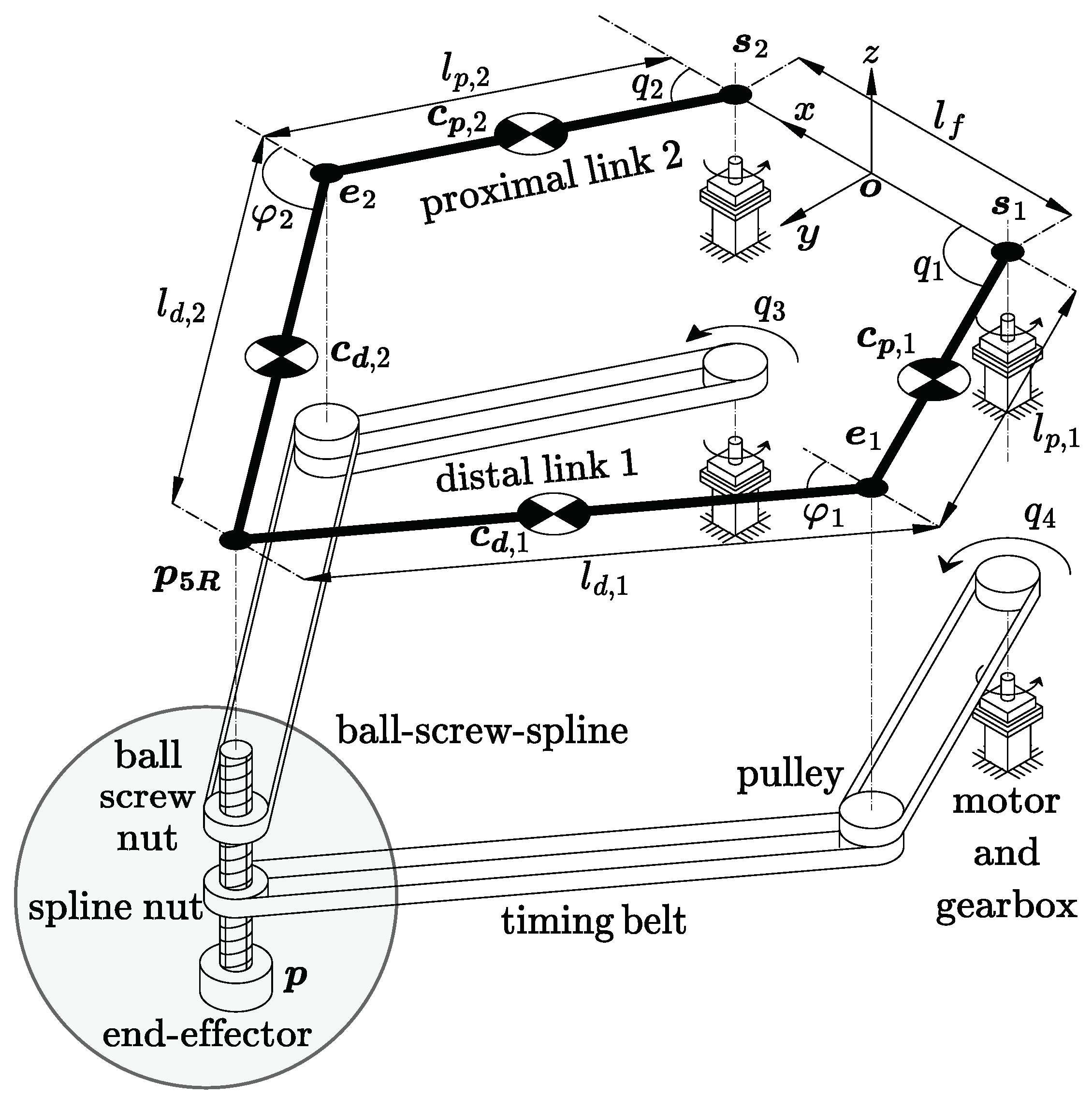
Section 2 presents the dynamic and the kinematic model of the robot object of the investigation (
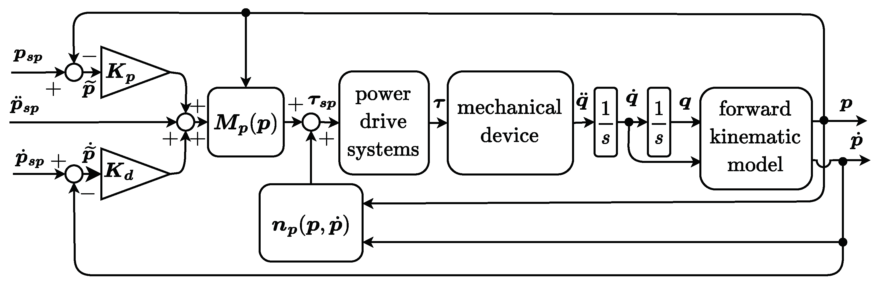
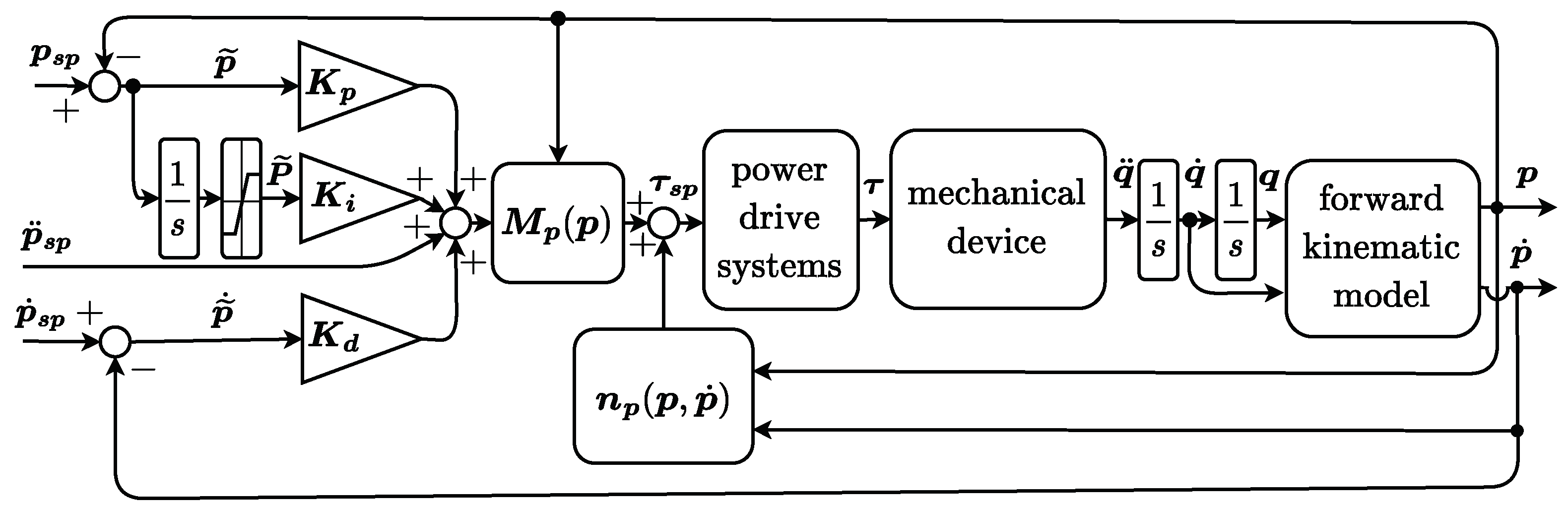
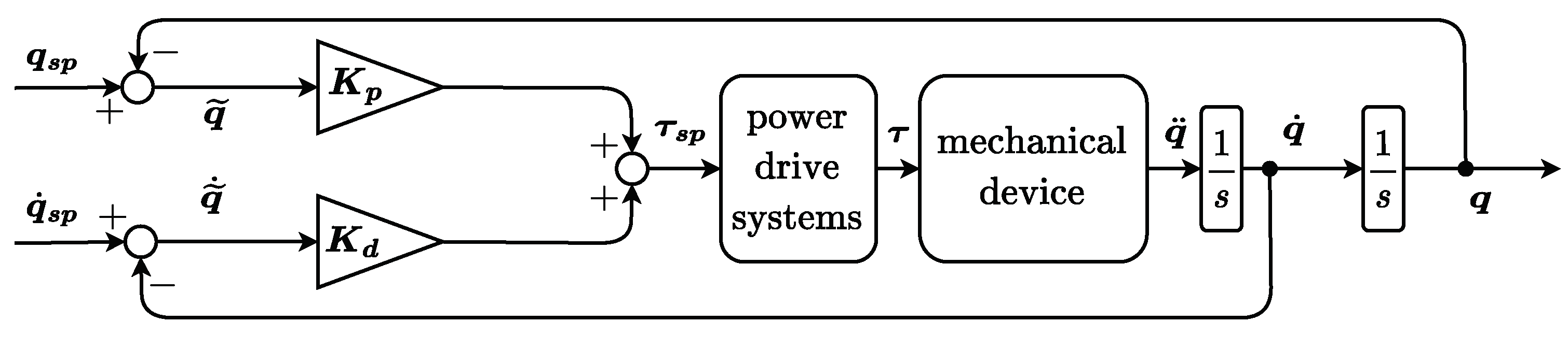
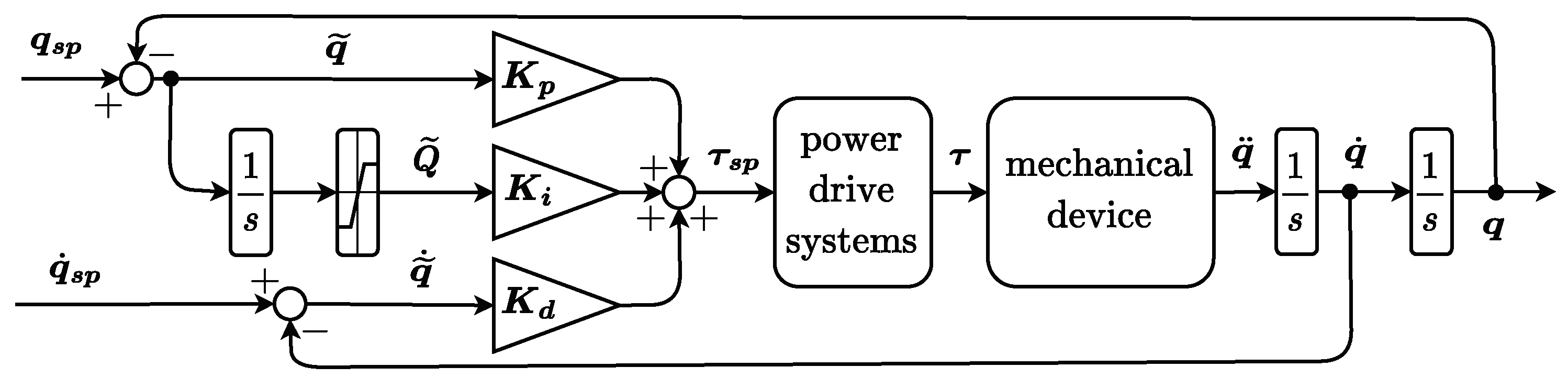
Section 2.1), the control schemes (Section 2.2), the reference pick-and-place task (
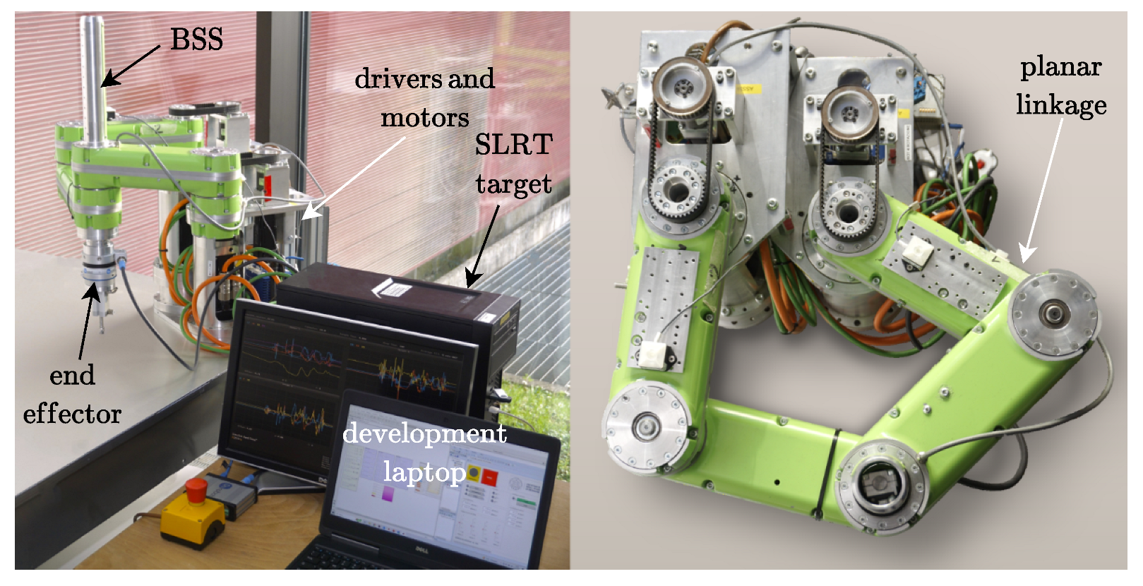
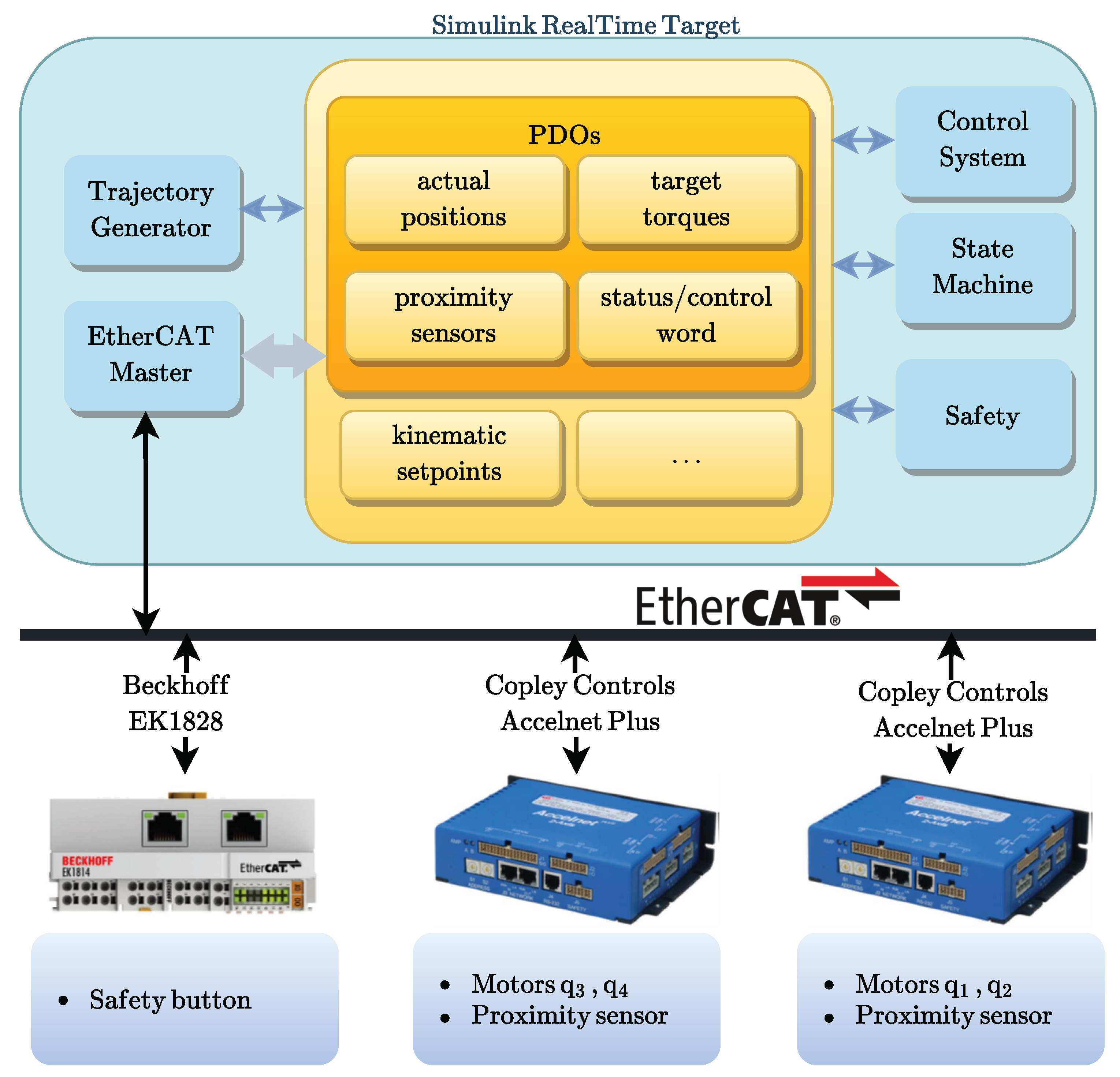
Section 2.3), and the software and hardware equipment (Section 2.4) used for the experimental activities. Section 3 discusses the collected experimental results and compares the investigated controllers’ performances. Finally, some conclusions are drawn in Section 4.

2. Methods

2.1. Dynamic Model of the Manipulator

The considered robot is a 4-DOF parallel kinematic manipulator designed for fast pick-and-place applications. As shown in Figure 1, the robot’s mechanical structure is composed of the following two main subsystems: a 5R planar linkage, which determines the position of point p 5 R in the horizontal plane, and a ball-screw-spline (BSS) mechanism mounted in p 5 R that enables the roto-translation of the end-effector along and around the vertical axis. The manipulator presents significant masses and inertias distributed among its main constitutive elements, marking a difference with other notable PKM architectures, such as the Delta robot, whose main masses are concentrated in a few key components. To counterbalance the presence of considerable masses, the mechanical design favoured high structural stiffness, in contrast, e.g., with the PKM investigated in [18].
All the parameters needed to describe the geometry, the mass distribution and the actuators of the device are determined during its mechatronic design phase, and can therefore be also used for the synthesis of the control system. The geometrical and mass parameters are in particular listed, described, and quantified in Table 1, with symbols and nomenclature consistent with those indicated in Figure 1. The numerical values of each quantity were provided by the manufacturer, Mechatronics and Dynamic Devices s.r.l., Dalmine, Italy [19]. The properties of the actuation systems are reported, on the other hand, in Table 2, the selection of the transmission and of the power drive systems having been performed according to the procedure detailed in [20].
The planar linkage is actuated by two servoaxes constituted each by a brushless motor and a planetary gearbox attached to the robot’s fixed frame. The BSS is actuated by another pair of similarly constituted servoaxes, through two timing belt transmission systems housed inside the hollow links. The pulleys constituting the transmissions have all the same radius; as a result, the BSS and the planar 5R mechanism are kinematically decoupled. In fact, the configuration of the 5R linkage is a function only of generalized coordinates q 5 R = q 1 q 2 , which, as shown in Figure 1, represent the proximal link rotations. Conversely, the configuration of the BSS is described by the joint coordinates q bss = q 3 q 4 , which ultimately correspond to the rotations of the ball screw and spline nuts that constrain the ball-screw-spline. As a result, the in-plane position p 5 R of the end-effector is determined exclusively by q 5 R , whereas its vertical and angular positions z e e and φ e e are functions of q bss only.
For motion planning purposes, it is useful to study the forward and inverse kinematics of the device up to the accelerations. A dynamic model of the robot is on the other hand useful for the development of centralized regulators.
The kinematics of the two mechanical subsystems is well-known and easily composed. The authors have already treated, in greater detail, the kinematics of the manipulator in [21]. An in-depth discussion of the singularities for the five-bar linkage can be found in [22,23], even though it should be remarked that the case study presented in this work does not involve the crossing of any singularity. Finally a more detailed discussion of the kinematics and dynamics of the 5R robot can be found in [14]. The dynamics of the entire mechanism may be written as follows:
M 5 R 0 0 M bss + M act q ¨ 5 R q ¨ bss + C 5 R 0 0 0 q ˙ 5 R q ˙ bss + 0 U b s s = τ ,
or more compactly as follows:
M ( q ) q ¨ + C ( q , q ˙ ) q ˙ + U = τ .
In Equation (1) M 5 R and M bss are the mass matrices associated with the planar linkage and to the BSS, respectively, C 5 R is the 5R ’s Coriolis and centrifugal actions matrix; U b s s is the gradient of the gravitational potential associated with the ball-screw-spline, while τ are the torques applied at the output shaft of the four gearboxes. It should be noted that the planar linkage operates in the horizontal plane, and hence its potential energy is constant; also it may be remarked that the BSS is a linear time-invariant system and, therefore, not subject to Coriolis and centrifugal actions. Finally, the following matrix:
M act = diag i t 1 2 ( J m 1 + J t 1 ) i t 2 2 ( J m 2 + J t 2 ) i t 2 2 ( J m 2 + J t 2 ) i t 4 2 ( J m 4 + J t 4 )
accounts for the effects of the moments of inertia J m j and J t j (with j = 1 , , 4 ) associated with the four motor shafts and gearboxes, considering as appropriate the reduction ratios i t j . The matrix M 5 R can be written as follows:
M 5 R = k = 1 2 m p , k D c p , k D c p , k + m d , k D c d , k D c d , k + J d , k D φ d , k D φ d , k + m e e D 5 R D 5 R + J p
with the following:
J p = J p , 1 0 0 J p , 2 .
In Equation (4) D c p , k and D c d , k represent the Jacobian matrices associated with the centers of mass of the proximal and distal links; D φ d , k indicate the Jacobian matrices of distal angles φ d , k , while D 5 R is the Jacobian of p 5 R . The mass and inertial parameters can all be found in Table 1 with their description and quantification. The matrix C 5 R has been written as follows:
C 5 R = k = 1 2 m p , k D c p , k D ˙ c p , k + m d , k D c d , k D ˙ c d , k + J d , k D φ d , k D ˙ φ d , k + m e e D 5 R D ˙ 5 R ,
exploiting the fact that the 5R linkage undergoes purely planar motions. In Equation (6), it can be seen that the time derivatives of the Jacobian matrices also appear. Fully working out these kinematic quantities is outside the scope of this work; moreover, they all have been determined exactly using as appropriate analytical and geometrical methods.
The kinematics of the BSS is invariant with respect to the joint configuration, and is thus fully described by a constant Jacobian matrix. Let p b s s be the pitch of the ball-screw-spline; the following kinematic relationships hold:
z ˙ e e φ ˙ e e = 1 2 π p b s s p b s s 0 2 π q ˙ bss = D bss q ˙ bss .
The kinetic and potential energies of the ball-screw-spline can therefore be expressed with respect to the joint variables as follows:
T b s s = 1 2 ( J 3 + m e e p b s s 2 4 π 2 ) q ˙ 3 2 + ( J 4 + m e e p b s s 2 4 π 2 + J e e ) q ˙ 4 2 m e e p b s s 2 2 π 2 q ˙ 3 q ˙ 4
U b s s = m e e g p b s s 2 π ( q 4 q 3 ) ,
where J 3 and J 4 are the moments of inertia of the ball screw and spline nuts (inclusive also of the inertia of the associated pulleys), m e e and J e e are the mass and moment of inertia of the end-effector, and g is the gravitational constant.
The mass matrix of the BSS can be obtained as the Hessian of T b s s with respect to q ˙ bss ; it results as follows:
M bss = ( J 3 + m e e p b s s 2 4 π 2 ) m e e p b s s 2 4 π 2 m e e p b s s 2 4 π 2 ( J 4 + m e e p b s s 2 4 π 2 + J e e ) .
The gradient of the potential energy U b s s is also straightforwardly computed as follows:
U b s s = m e e g p b s s 2 π 1 1 ,
It should be noted that this kind of mathematical modelling neglects the elasticities of the belt transmission systems. These could be modelled using an appropriate elastic potential energy function, which, however, would require the introduction of additional non-actuated and non-measured degrees of freedom.
Considering again the entire system, the Jacobian matrix that relates the time derivatives of the joint coordinates to the end-effector velocity can be written block by block as follows:
D = D 5 R 0 0 D bss .
Consequently its time derivative assumes the following form:
D ˙ = D ˙ 5 R 0 0 0 .
Equation (2) represents the classical description of the dynamics of the system expressed in the joint space. Given the goal of developing centralized control systems operating with task space variables, the equations of motion of the entire system can also be rewritten as follows:
M ( p ) D 1 ( p ¨ D ˙ D 1 p ˙ ) + C ( p , p ˙ ) D 1 p ˙ + U ( p ) = τ .
Finally, through the suitable collection of the relevant terms it becomes possible to write the task space formulation of the following equations of motion:
M p ( p ) p ¨ + n p ( p , p ˙ ) = τ .
This last form is the one used for the development of the centralized control systems described in the following section:

2.2. Control Schemes

In this work, a modern model-based approach to the development of the robot’s control system is adopted, whereby the synthesis of the regulator uses all the information commonly available from the device’s overall mechatronic design. As a result, the detailed knowledge of the geometric and mass properties of the system, already included into its kinematic and dynamic models, is furthermore leveraged to improve the control performance. The proposed controllers are therefore of the inverse dynamic type, and are directly synthesized in the task space. The first one features only proportional and derivative feedback; as detailed below, the second also includes integral actions. These controllers are experimentally investigated and characterized through comparison with two joint space decentralized controllers of the PD and PID types, which, due to their widespread use, constitute useful benchmarks. The centralized control systems are based on task space variables and, in principle, allow the designer to directly specify the desired dynamics of the end-effector position error p ˜ = p sp p (with p sp being the setpoint and p the actual end-effector position). Figure 2 represents one of these regulators, the task space inverse dynamics controller (TSIDC). Its centralized nature stems from the following properties:
  • Both the mass matrix M p of the system and the feedback linearization term n p are computed as a function of the four task space coordinates of the system according to the dynamic model expressed in Equation (15);
  • Each torque setpoint is calculated according to the errors on more than one coordinate, since the mass matrix is not purely diagonal.
Considering, in particular, diagonal matrices K p and K d , the torque setpoint is determined according to the following equation:
τ sp = M p ( p ) ( p ¨ sp + K d p ˜ ˙ + K p p ˜ ) + n p ( p , p ˙ ) ,
in which several torque components can be singled out and defined as follows:
τ p ( TSID ) = M p K p p ˜
τ d ( TSID ) = M p K d p ˜ ˙
τ M p ( TSID ) = M p p ¨ sp
τ n p ( TSID ) = n p ( p , p ˙ ) .
The torque setpoint τ sp is saturated in relation to the maximal performances achievable by the power drive systems and then fed into the driver, which generates the actual torque τ .
Assuming a perfectly matched dynamic model of the system and as a first approximation an identity between τ and τ sp , substitution of Equation (16) into Equation (15) leads to the task space error dynamics equation in the form p ˜ ¨ + K d p ˜ ˙ + K p p ˜ = 0 , in which K p and K d can be selected, e.g., through pole placement.
However, the feedback linearization of the system is imperfect due to unmodelled effects such as friction actions and non-idealities of the inner torque control loops; as a result, the actual error dynamics remains excited by a residual disturbance term d appearing on the right-hand side, and do not, in practice, converge to zero as follows:
p ˜ ¨ + K d p ˜ ˙ + K p p ˜ = d .
To counteract this effect several strategies have been proposed in the literature, ranging from adaptive control schemes [24,25,26,27], to sliding mode robust controllers [28,29,30,31]. The present paper investigates a centralized control strategy in which an integral contribution is added to the base TSID regulator, yielding the task space integral inverse dynamics controller (TSIIDC); its block diagram is represented in Figure 3. The integrator is implemented as a discrete time-forward Euler accumulator, which temporarily stops its summation whenever an upper or lower bound has been reached. This overall behaviour, which prevents the windup of the integral term, is indicated with slight abuse of notation in Figure 3 by the saturation symbol. Since the TSIIDC works in the task space, the output of the accumulator, denoted as P ˜ , is closely related to the integral of the task space position errors. The overall equation that yields the torque setpoint is as follows:
τ sp = M p ( p ) ( p ¨ sp + K d p ˜ ˙ + K p p ˜ + K i P ˜ ) + n p ( p , p ˙ ) ,
where again K p , K d and also K i are diagonal matrices. From Equation (22) several torque contributions may be isolated as follows:
τ p ( TSIID ) = M p K p p ˜
τ d ( TSIID ) = M p K d p ˜ ˙
τ i ( TSIID ) = M p K i P ˜
τ M p ( TSIID ) = M p p ¨ sp
τ n p ( TSIID ) = n p ( p , p ˙ ) .
The error dynamics in this case assumes the following form:
p ˜ ¨ + K d p ˜ ˙ + K p p ˜ + K i P ˜ = d .
Figure 4 depicts the PD regulator. Given the joint position and velocity setpoints q sp , q ˙ sp , the joint position and velocity errors q ˜ = q sp q and q ˜ ˙ = q ˙ sp q ˙ are computed and used to generate a torque setpoint τ sp according to the following relationship:
τ sp = K d q ˜ ˙ + K p q ˜ = τ d ( PD ) + τ p ( PD ) .
Even though Equation (29) is written in vector form, it should be noted that the control loop of each joint is completely independent from the others owing to the fact that the matrices K d and K p are diagonal. The PID controller, illustrated in Figure 5, features an additional feedback action operating on the integral of the joint position error. The implementation of the integrator is analogous to the one already described for the TSIIDC, with its output being denoted as Q ˜ ; as can be inferred from the figure, the equation associated with the PID regulator is as follows:
τ sp = K d q ˜ ˙ + K p q ˜ + K i Q ˜ = τ d ( PID ) + τ p ( PID ) + τ i ( PID ) .
Again Equation (30) is written in vector form, but since K d , K p , and K i are diagonal matrices the PID control loops operate without interactions between each other.

2.3. Workcycle Description

The regulators are tested on a workcycle generated by the motion planning system previously developed by the authors [21] specifically to define fast pick-and-place operations on moving objects such as items carried by conveyor belts. The trajectory is first defined geometrically, taking into account the shape of the singularity-free workspace of the 5R manipulator; subsequently the position, velocity, and acceleration setpoints are generated as a function of time, taking care to minimize the overall execution time of the trajectory given the constraints determined by the physical properties of the robot and of its actuation systems.
Figure 6 illustrates the workcycle used as a test case. The path, expressed in the task space coordinates, is represented in the foreground, with the color indicating the value of the end-effector rotation. In the background, the outline of the two conveyor belts that are envisioned for this type of application is represented in green, and the footprint of the useful workspace of the robot is also represented by the black line. The red markers placed on the trajectory and labelled from (a) to (i) divide the overall pick-and-place cycle into its constitutive phases. These are as follows:
  • (a)–(b): Pick intercept motion that brings manipulator’s end-effector directly above and aligned with its target item; at point (b) the velocity of the robot matches that of the pick conveyor;
  • (b)–(c): Descent motion that brings the end-effector in contact with the item to be picked; during this phase the velocity of the conveyor belt is tracked in the longitudinal direction;
  • (c)–(d): Grasping motion, during which the conveyor velocity is tracked as the gripping tool on the end-effector operates to collect the item;
  • (d)–(e): Ascent motion, in which the end-effector moves away from the conveyor while still tracking its longitudinal velocity to avoid any collision with other items on the belt;
  • (e)–(f): Intercept motion needed to reach the moving place position (e.g., an empty box carried by the place conveyor);
  • (f)–(g): Descent motion, in which the item held by the robot is lowered to the level of the place conveyor;
  • (g)–(h): Deposit motion, in which the item is released on the conveyor;
  • (h)–(i): Ascent motion;
  • (i)–(a): Auxiliary deceleration motion that brings the robot to a resting state.
From the description above it is clear that a full pick-and-place cycle is composed of two similarly structured halves, each constituted by a target intercept motion followed by a conveyor tracking movement. The conveyor tracking phase is itself subdivided into the descent movement, the item grasping or release, and the ascent motion.
The task space setpoints are represented as a function of time in Figure 7, at the position, velocity, and acceleration levels. The gray areas highlight the conveyor tracking phases, whereas the remaining portions correspond to the fast target intercept motions.
All included, the full pick-and-place cycle lasts 2.46   s ; a peak linear velocity of 1.16   m / s is reached, whereas the peak linear acceleration is equal to 11.3 m s−2. Concerning the workcycle geometry, it can be seen in Figure 6 that it occupies a large portion of the useful workspace. The more dynamic portions of the workcycle are constituted by the target intercept motions, during which the end-effector should quickly reach its destination; within these phases the setpoint tracking accuracy is not paramount, while the attainment of high speed is more important given the need to reduce the cycle time. As will be shown in the following section, the required torques are quite significant during these phases, and briefly reach the saturation levels, which were set to the maximal torque compatible with the power drive systems. Torque saturations were purposefully allowed in order to ensure the full exertion of the system’s dynamic capabilities. On the contrary, the conveyor tracking motions are performed at a lower and constant end-effector velocity, compatible with typical industrial applications. In these portions of the workcycle, the manipulator should accurately track the conveyor and guarantee high precision, due to the finer nature of the grasping and release operations. Therefore, the proposed test cycle covers a wide range of situations, and allows the investigation both of highly dynamic working conditions, characterized by high accelerations and velocities, and of the quasi-stationary motions experienced during the conveyor tracking phases.

2.4. Experimental Setup

In Figure 8, the experimental setup of the manipulator is shown. In the figure, the following elements are highlighted: the mechanical structure of the robot, with its two subsystems (the planar linkage and the BSS); the actuation systems; the desktop computer on which the control algorithms are executed; and the laptop used for software development. All computations were implemented in Matlab/Simulink 2017a.
In the Figure 9, a schematic of the software and communication architecture is shown. The system consists of the following two macro-components: the Simulink Real-Time (SLRT) target and the EtherCAT field bus with its connected slaves.
The SLRT target is a computer that handles all the control logic of the system, relying on the services provided by the Simulink Real-Time operating system. Figure 9 schematizes the main components of the developed Simulink program, which features the following:
  • The state machine, which implements the main operating logic;
  • The safety logic subsystem protecting the experimental setup from user or programming errors;
  • The EtherCAT communication Master, natively included in Simulink Real-Time, which deals with communication from and to the field devices;
  • The implementation of the previously described controllers.
Figure 9 depicts the complete EtherCAT network needed to exchange data between the EtherCAT master and the field devices (drivers and digital inputs and outputs). The Simulink Real-Time target and the EtherCAT network have been set up to operate at a sampling frequency f s equal to 4 kHz. The resulting sampling time T s = 0.25   m s determines the deadline that the control systems must meet for all their computations, which, in the case of the TSIDC and TSIIDC, involve the full evaluation of the robot’s kinematic and dynamic models.
Two key elements of the experimental setup are the two Accelnet BE2-090-20-R drivers, each capable of controlling two brushless motors using different operating modes and configured as EtherCAT slaves. Since the developed control schemes are all conceived to directly generate the torque setpoints, the drivers have been set up to work in torque mode.

3. Results and Discussion

In this section, the main experimental findings related to the performance of the task space centralized controllers are reported and discussed also through comparison with the joint space PD and PID controllers. Some of the reported results concern the entire workcycle, whereas others focus solely on the higher speed second half of the pick-and-place cycle in order to present an uncluttered overview of the main findings. Whenever this distinction is not immediately evident, it is made explicit in the course of the discussion. The tests were performed through the execution of the workcycle described in Section 2.3, once for each controller. The quantities of interest were logged using the functionalities offered by the Simulink Real-Time operating system, and subsequently post-processed and organized in the graphical form presented in the following discussion. The controllers were tuned using different procedures according to their type. For the TSIDC, the gains are such that the dynamics of the in-plane error components nominally have poles at 30 Hz with damping of 0.7 , whereas those of the remaining ones have poles placed at 28 Hz , with a damping of 0.6 . The integral gains of the TSIIDC were, on the other hand, experimentally tuned, leaving the proportional and derivative gains unaltered. 
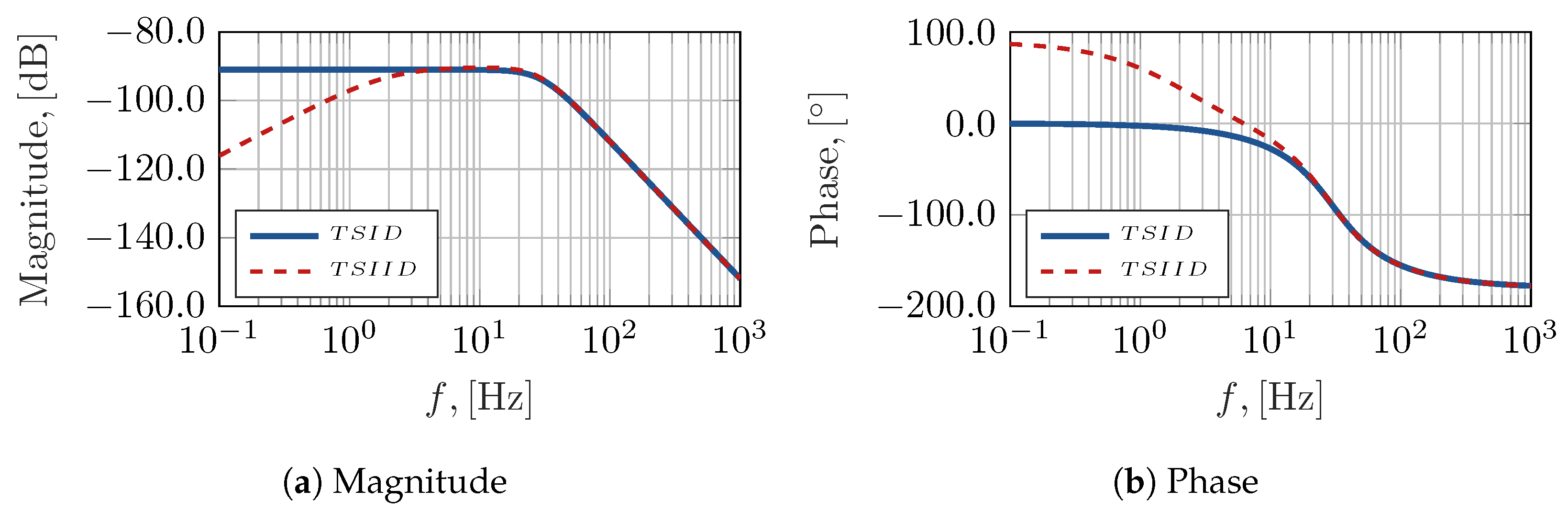
Figure 10 shows the transfer functions from the torque disturbances to the task space in-plane position errors achieved with the TSID and TSIID controllers; in particular, from Figure 10a it can be observed that the introduction of the integral term improves the rejection of the disturbance’s low frequency components.
The decentralized controllers’ parameters, being less amenable to clear interpretation and representation, were selected with ad hoc tuning aiming at the maximization of the regulator’s performance. 
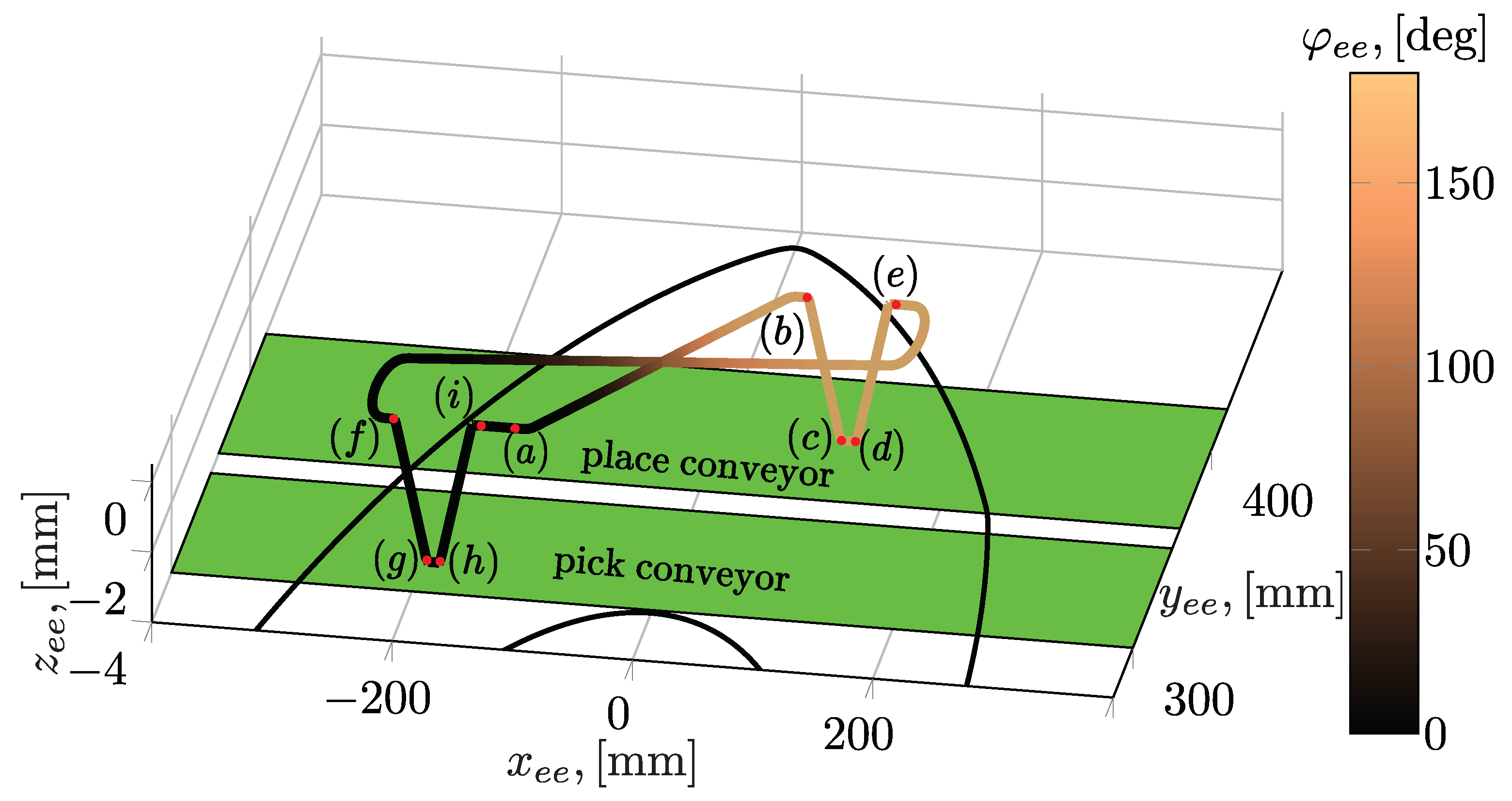
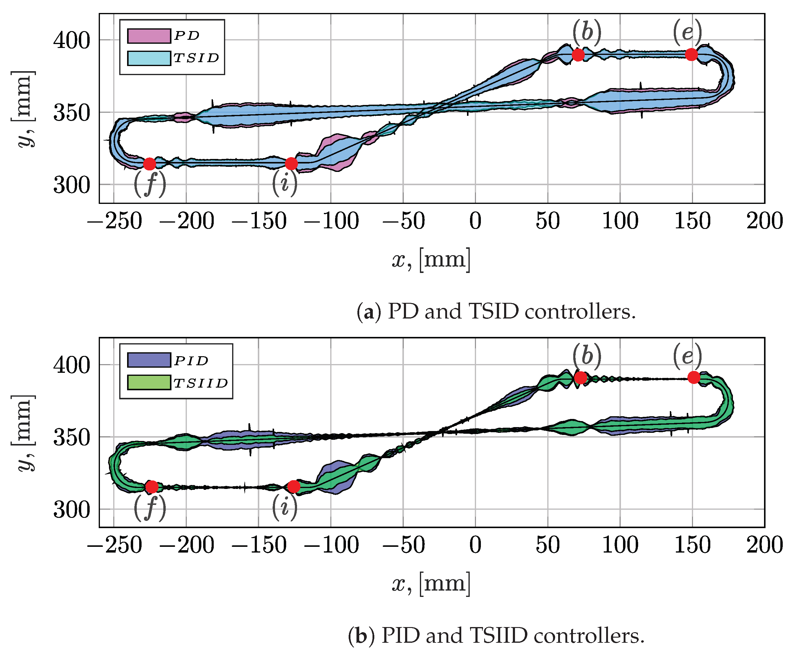
Figure 11 shows the norm of the errors on the horizontal plane, projected along the normal direction of the path and magnified by a factor of 20. The path, whose planar projection is shown in the figure, coincides with the one reported in Figure 6, and described in detail in Section 2.3. Here, it may be remarked that the conveyor tracking phases take place between points (b)–(e) and (f)–(i), whereas the remaining portions of the trajectory are fast intercept motions. Figure 11a in particular shows the errors achieved using the PD and TSID controllers, whereas Figure 11b depicts the errors obtained using the PID and TSIID controllers. It can be seen that the TSID controller generally performs better than the PD regulator, similarly, the TSIIDC outperforms the PID controller. It therefore appears that the introduction of model-based components is beneficial irrespectively of the presence of an integral term. Through the comparison of Figure 11a to Figure 11b it can be concluded that, in general, the introduction of an integral control action leads to significant performance improvements, especially in those phases of the workcycle that are characterized by low accelerations (i.e., the conveyor tracking phases (b)–(e) and (f)–(i), along with the central portions of the intercept motions).
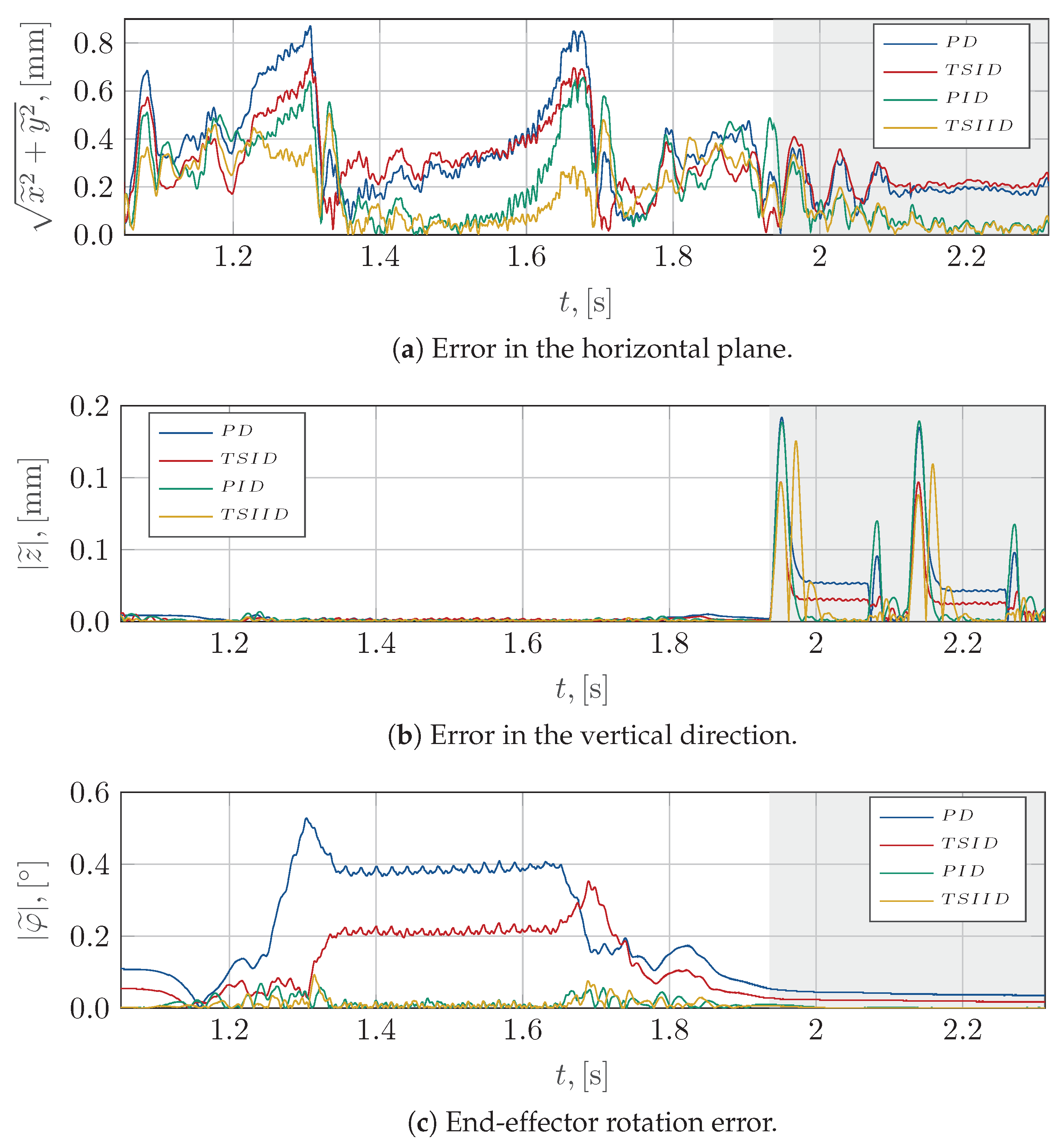
Figure 12 presents the position errors in the time domain, focusing on the second half of the workcycle; the gray area highlights the tracking phase; the same convention is adopted also for subsequent figures. Figure 12a is clearly consistent with the results already presented in Figure 11, whereas Figure 12b,c confirm the analysis above also in relation to the vertical translation and rotation errors. In particular, in Figure 12b, it can be seen that during the conveyor tracking phases, where the z e e setpoint is not constant, both the PD controller and the TSIDC lead to relatively large errors, with the TSIDC performing better than the PD regulator. On the contrary, the controllers having an integral contribution are better able to bring the error along the vertical direction to zero. The TSIIDC error displays, however, a more oscillating behaviour compared both to the decentralized controllers and to the TSIDC.
In Figure 12c, it can be seen that during the intercept motions, where the end-effector should perform a 180 ° rotation, the PD regulator and the TSIDC lag behind the setpoint; additionally, they are unable to bring the error to zero also during the ensuing tracking phase, where the end-effector does not rotate anymore. A significantly better behaviour is instead achieved through the introduction of the integral component, with the PID controller and the TSIIDC performing equally well. 
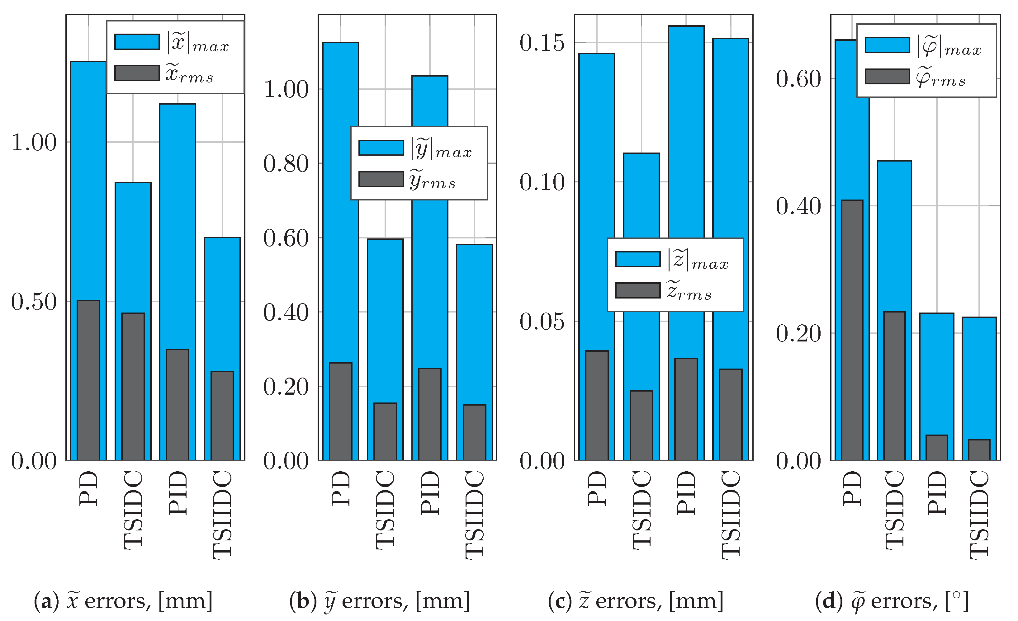
Figure 13 presents the achieved peak and RMS errors computed along the entire workcycle, for each end-effector coordinate and for each controller. This kind of global representation has not been commonly found in the reviewed literature, which focuses mostly on the errors’ time history; however, these synthetic indices are also useful to compare at an aggregate level to the performance of the controllers. Concerning the peak | x ˜ | m a x and | y ˜ | m a x errors, an analogous trend can be discerned, namely, the centralized controllers are able to markedly reduce them. Along the x direction, the introduction of an integral term appears to be useful to reduce the RMS error, as the PID and TSIID controllers outperform the remaining two. On the other hand, along the y direction the best performers in terms of the RMS errors are the two centralized controllers. The peak and RMS z ˜ errors seem to suggest that, in aggregate terms, the best performer is the TSID regulator; however, a review of Figure 12b shows that the controllers that also feature an integral term are better able to bring the error to zero in quasi-stationary conditions, occurring, e.g., during the release or grasping phases. As can be seen in Figure 13d, the rotational error φ ˜ , both in peak and RMS values progressively improves going from the PD to the TSID and then to the PID and TSIID controllers. It is possible to deduce that for this coordinate, the introduction of an integral term is the most important factor as follows: indeed, notwithstanding the fact that the TSID controller significantly outperforms the PD regulator, further non-negligible improvements are achieved in almost equal measure by the PID and TSIID controllers.
The articles reviewed in the introduction seldom report a measure of the control torques (or currents), with the greatest focus being only on the achieved errors. On the contrary, in this work, not only the overall control torques but also their constitutive components are highlighted, both instantaneously and at the aggregate level. This is done in order to clearly show how each controller operates, and which components of the control systems are actually relevant during the different phases of the test workcycle. In fact, a peculiarity of the case study presented here is the alternation of highly dynamic motions in which inertial forces dominate and of the almost constant velocity phases during which static and viscous friction is expected to act as a relevant source of disturbance.
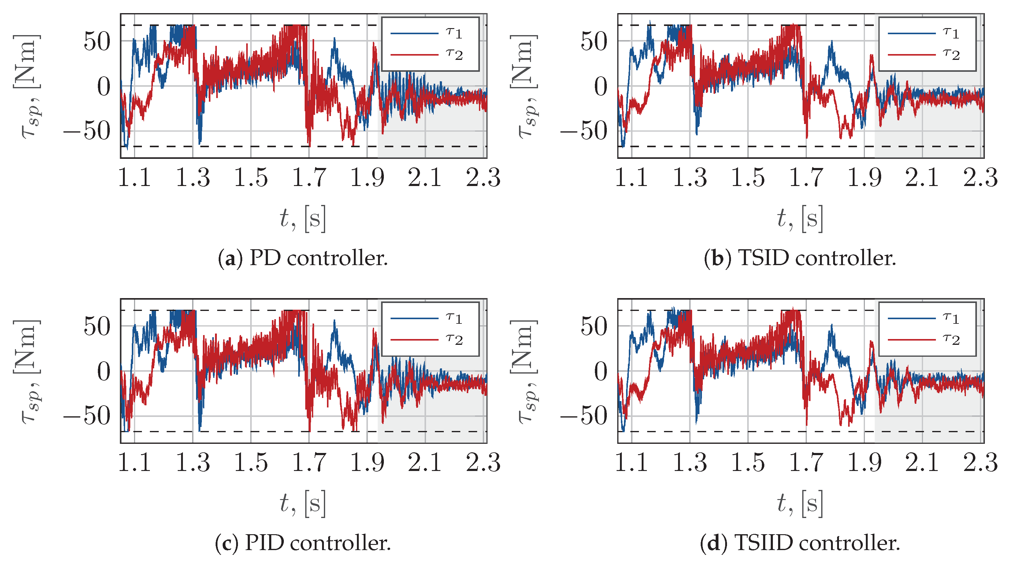
 Figure 14 and Figure 15 illustrate the torque setpoints generated by each controller, respectively, at the motors actuating the joint coordinates q 1 , q 2 and q 3 , q 4 . As already introduced, the possibility of short-term torque saturation was purposely allowed to ensure that the behaviour of the system is investigated up to maximally challenging conditions. Concerning Figure 14, it can be seen that the overall behaviour is very similar for all controllers, with torque saturations also being reached in all cases around times 1.25 s and 1.65 s. A close inspection reveals that for the centralized controllers, the saturations have a slightly lower duration, and also the remaining torque peaks are less pronounced. The saturations tend to be correlated on the one hand with the in-plane error peaks, and on the other with higher setpoint accelerations.
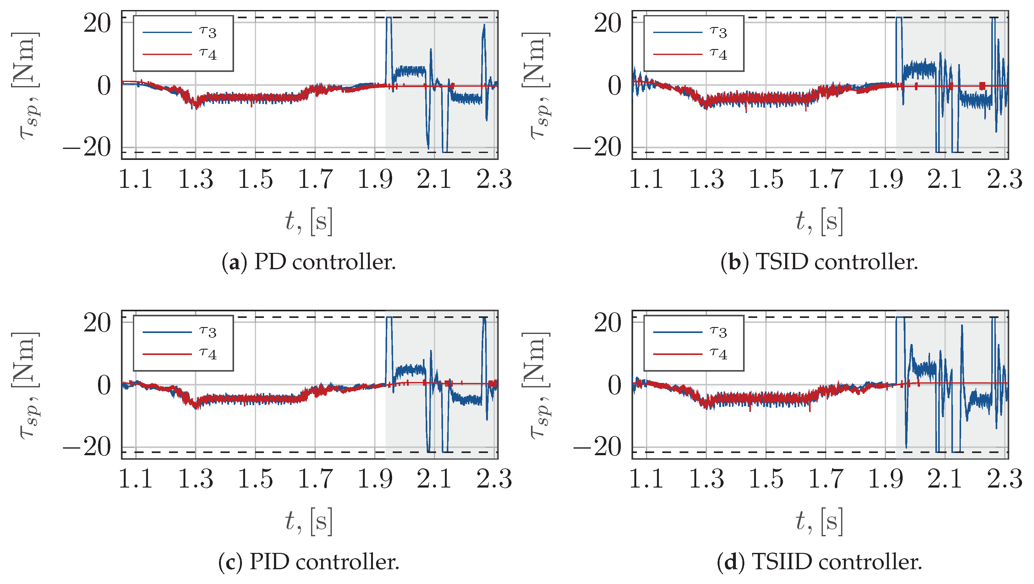
Figure 15 shows that during the target intercept phase, the motors actuating the q bss joints are not under particular strain; conversely, in the conveyor tracking phase, especially along the vertical descent and ascent motions, motor torque τ 3 has a tendency to reach its saturation value. The behaviour of the four regulators is similar in this respect; however, the torque τ 3 generated by the centralized controllers displays more marked oscillations. Figure 16, Figure 17, Figure 18 and 
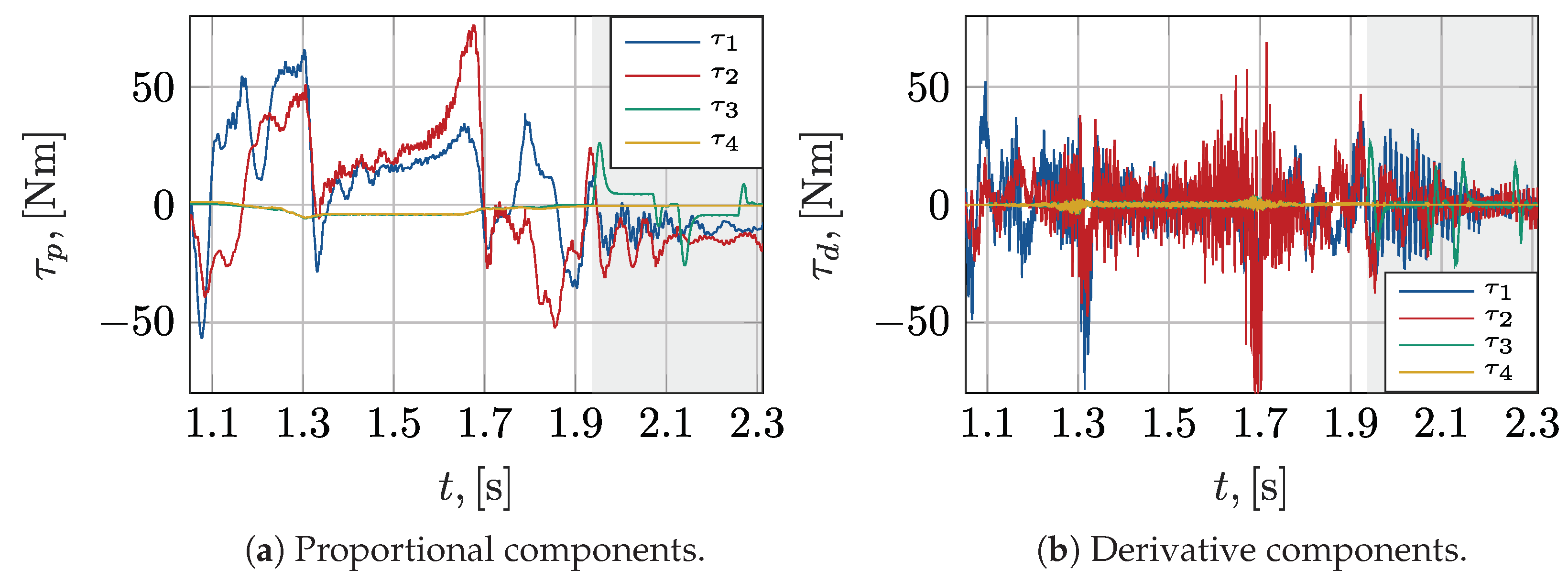
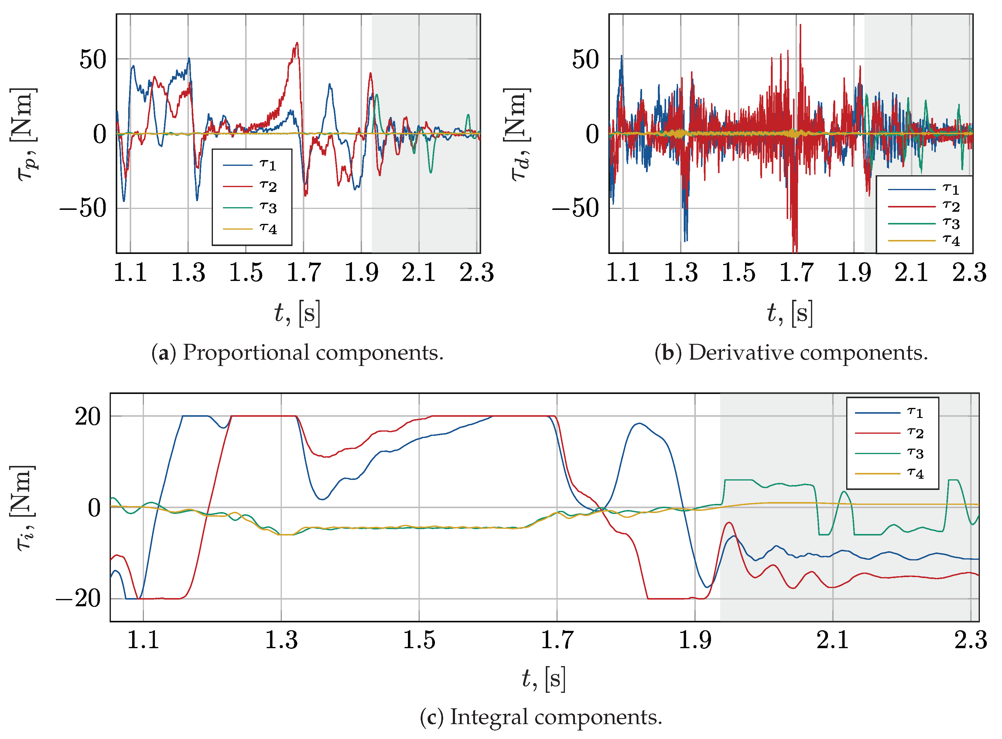
Figure 19 show the several components that contribute to the overall torque setpoint generated by each controller. These torque components are represented without considering the global saturations, since the ability to clearly tell them apart would be otherwise impaired. Comparing Figure 16 to Figure 17, it can be clearly seen that the proportional components are not distributed, in the case of the PD controller, around the zero level. Conversely, in the case of the PID controller, the proportional terms, especially in the portions of the trajectory characterized by less pronounced accelerations, decay to or oscillate around zero. This effect is due to the introduction of the integral actions, which successfully prevent, in the several sub-phases of the trajectory, the permanence of non-null position errors, while the overall torques are similar, they result as already commented in quite different error patterns. No significant differences emerge by the comparison between the derivative components of the PD and PID controllers.
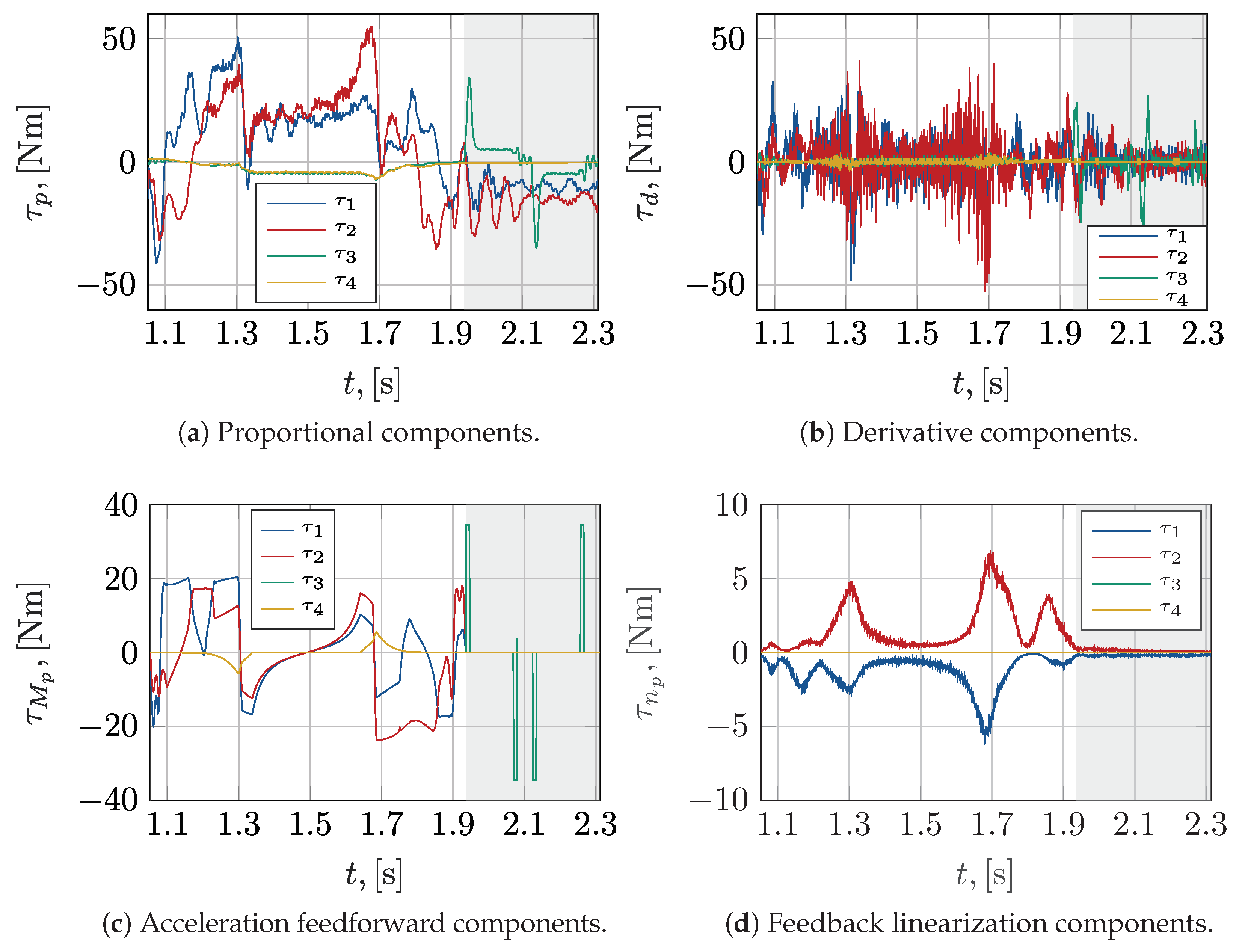
The joint analysis of Figure 18 and Figure 19 shows that, quite obviously, the τ M p , j and τ n p , j components are, respectively, exactly or practically the same for the TSID and TSIID controllers. The feedback linearization contributions τ n p , 3 and τ n p , 4 to torques τ s p , 3 and τ s p , 4 are almost null, and due exclusively to the almost negligible gravitational actions. Conversely, τ n p , 1 and τ n p , 2 do contribute to torques τ s p , 1 and τ s p , 2 , but significantly so only in the vicinity of the velocity peaks. Their entity is at any rate lower than the acceleration feedforward components τ M p , 1 and τ M p , 2 .
Comparing the proportional components of the PD and TSID controllers, and also observing the acceleration feedforward components τ M p , j , it is possible to ascertain that the peak values tend to occur synchronously, in the trajectory portions characterized by high accelerations. The acceleration feedforward components of the TSIDC appear to absorb part of the torque from the proportional terms, leading to the reduction in their peak values. As occurred for the PD regulator, also the proportional torque components of the TSIDC do not coalesce around zero, since position errors attributable to unmodelled friction actions persist also during quasi-stationary conditions.
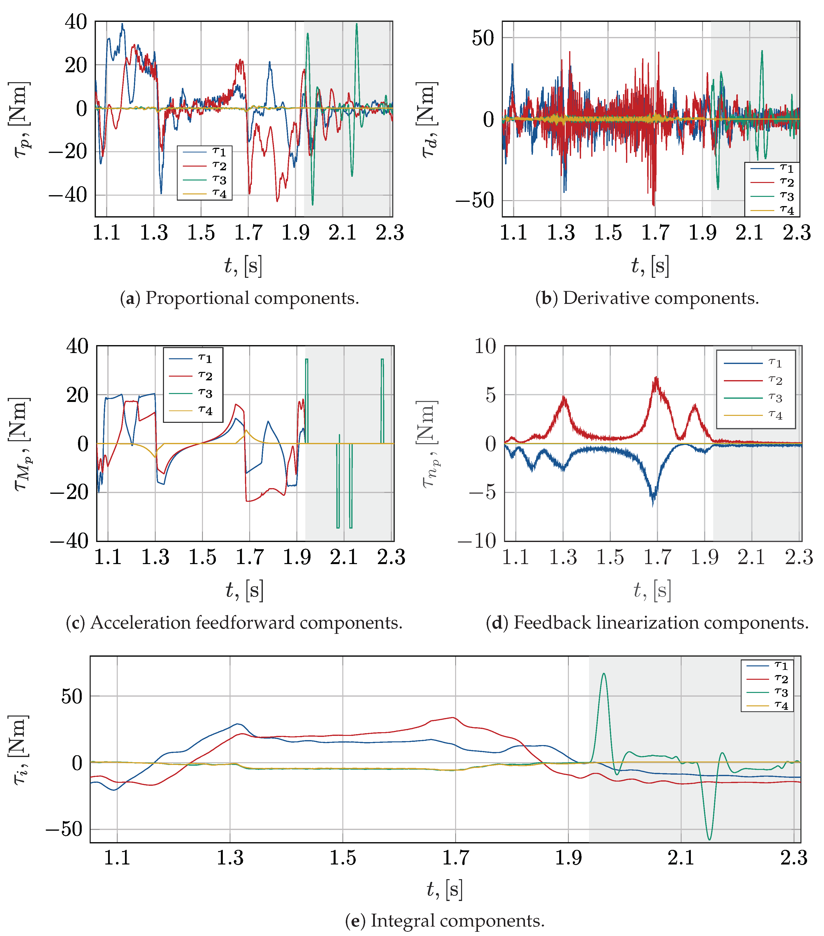
The introduction of the integral terms in the TSIIDC counteracts this effect, as these contributions absorb the low-frequency components of τ p ( TSID ) . The overall supplied torque remains largely unchanged, but the position errors induced by the unmodelled terms that characterize the actual robot’s dynamics are reduced. The adoption of centralized control methods finally appears to reduce the peak values of the components based on the velocity errors. 
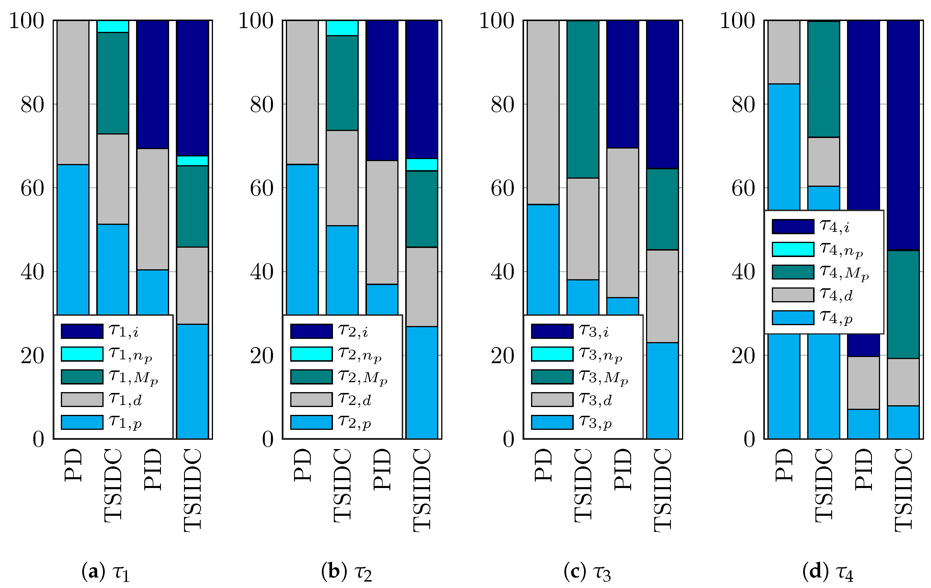
Figure 20 shows how the torque setpoints are divided into the different components at an aggregate level, over the course of the entire workcycle. In particular, the RMS values of each torque component were evaluated, and are expressed in the figure as a percentage of their overall sum. In Figure 20a,b, which concern, respectively, τ s p , 1 and τ s p , 2 , almost identical trends can be observed. Going from the PD regulator to the TSID and then to the PID and TSIID controllers, the proportional torque contribution is progressively reduced. The PID and TSIID controllers feature an integral term of roughly equal weight. The feedback linearization terms are of low entity in both the TSIDC and the TSIIDC. Using the PD as the base case, it can be observed that the derivative contributions decrease especially when control centralization is introduced, and conversely, are less affected by additional integral components. Similar considerations can be drawn from Figure 20c. In Figure 20d, which concerns the fourth degree of freedom, it is apparent that the integral contribution is especially important whenever it is introduced. In particular, for both the PID and the TSIID controllers, the proportional and derivative terms have a similarly low relevance.

4. Conclusions

In this work, centralized model-based controllers for a 4-DOF parallel kinematic robot are synthesized using the information derived from the mechatronic design of the entire system. Given the availability of an accurate characterization of the geometric and mass properties of the robot, which are established at design time, it is possible to build kinematic and dynamic models useful for control system development and for dynamic performance maximization. A task space formulation of the inverse dynamics control was first adopted and further refined through the introduction of an integral action term. The computational load stemming from the evaluation of the mathematical model of the robot was observed to be compatible with modern commodity hardware, despite the relatively high sampling frequency of 4 k Hz . The behaviour of the centralized controllers was experimentally characterized through the execution of a high-speed pick-and-place cycle representative of the robot’s intended use. One peculiarity of this application lies in the wide range of experienced working conditions, which alternate between highly dynamic motions and slower movements in which the accuracy requirements are stringent. Classic PD and PID regulators were also considered as benchmarks.
The TSIDC performed well during the high speed and high acceleration phases, but was unable to bring the errors to zero during the quasi-stationary motions due to disturbances arising from unmodelled friction actions. These were, therefore, counteracted through the introduction of an integral term, yielding the TSIID controller, which was found to be able to operate satisfactorily in both kinds of situation. The PD and PID decentralized regulators were reliably outperformed by their centralized counterparts. Moreover, despite their simple structure, their experimental tuning was found to be time consuming. On the contrary, the synthesis of the TSID and TSIID controllers required an undeniably more complex implementation, which, however, finds a natural collocation within the overall design of the mechatronic system. Once developed, moreover, their free parameters were tuned with lower effort thanks to their clear interpretability.
Based on these considerations, it can be stated that, for applications similar to the one presented in this paper, the use of a centralized controller and, in particular, of a TSIID controller, allows the system to achieve high positioning performances both in high dynamics operations and in semi-stationary conditions. The adoption of centralized controllers in general appears particularly advantageous whenever a high-confidence estimate of the main system parameters is available as a by-product of the device design process.
Moreover, the proposed investigation highlighted the several components that contribute to the control torques. The results show that, in general, the centralized control actions account for a sizable part of the overall generated torque, and are especially beneficial for the reduction in the peak errors; moreover, the integral action introduced within the TSIIDC also has a relevant weight and leads to significantly lower RMS errors. These findings suggest that while the inertial effects have been successfully compensated thanks to the dynamic model of the system, the friction actions are non-negligible terms within the actual mechanical dynamics. The authors therefore plan to specifically investigate this issue, with the overall goal of providing an alternative to the integral torque components in the form of a suitably derived friction model.

Author Contributions

Conceptualization, P.R. and F.C.; methodology, P.R., F.C., J.S. and F.T.; software, J.S., F.T. and F.C.; validation, F.C. and F.T.; investigation, P.R., R.S., F.C. and J.S.; resources, A.G.; writing—original draft preparation, P.R., R.S., F.C., J.S. and F.T.; supervision, P.R. All authors have read and agreed to the published version of the manuscript.

Funding

The research was funded by the University of Bergamo. Fund code: 60RIGH21.

Data Availability Statement

Data are contained within the article.

Acknowledgments

Authors thank the company Mechatronics and Dynamic Devices s.r.l. for the design and the realization of the robot.

Conflicts of Interest

Author Andrea Ginammi was employed by the company Mechatronics and Dynamic Devices s.r.l, Italy. The remaining authors declare that the research was conducted in the absence of any commercial or financial relationships that could be construed as a potential conflict of interest.

References

  1. Saied, H.; Chemori, A.; El Rafei, M.; Francis, C.; Pierrot, F. From Non-model-Based to Model-Based Control of PKMs: A Comparative Study. Mech. Mach. Sci. 2019, 58, 153–169. [Google Scholar] [CrossRef]
  2. Sancak, K.V.; Bayraktaroglu, Z.Y. Nonlinear Computed Torque Control of 6-Dof Parallel Manipulators. Int. J. Control. Autom. Syst. 2022, 20, 2297–2311. [Google Scholar] [CrossRef]
  3. Shang, W.; Cong, S. Nonlinear computed torque control for a high-speed planar parallel manipulator. Mechatronics 2009, 19, 987–992. [Google Scholar] [CrossRef]
  4. Vu, M.T.; Alattas, K.A.; Bouteraa, Y.; Rahmani, R.; Fekih, A.; Mobayen, S.; Assawinchaichote, W. Optimized fuzzy enhanced robust control design for a Stewart parallel robot. Mathematics 2022, 10, 1917. [Google Scholar] [CrossRef]
  5. Tajdari, F.; Ebrahimi Toulkani, N. Implementation and intelligent gain tuning feedback–based optimal torque control of a rotary parallel robot. J. Vib. Control 2022, 28, 2678–2695. [Google Scholar] [CrossRef]
  6. Hu, H.; Chen, S.; Zhao, J.; Luo, J.; Jia, S.; Zhou, J.; Zhang, J.; Xiong, C.; Zhang, C.; Yang, G. Robust Adaptive Control of a Bimanual 3T1R Parallel Robot with Gray-Box-Model and Prescribed Performance Function. IEEE/ASME Trans. Mechatron. 2024, 29, 466–475. [Google Scholar] [CrossRef]
  7. Wu, G.; Lin, Z. On the Dynamics and Computed Torque Control of an Asymmetric Four-Limb Parallel Schonflies Motion Generator. J. Robot. Autom. 2020, 4, 168–178. [Google Scholar] [CrossRef]
  8. Lin, Z.; Cui, C.; Wu, G. Dynamic modeling and torque feedforward based optimal fuzzy pd control of a high-speed parallel manipulator. J. Robot. Control 2021, 2, 527–538. [Google Scholar] [CrossRef] [PubMed]
  9. Fontes, J.V.D.C.; Colombo, F.T.; Silva, N.B.F.D.; Silva, M.M.D. Model-based joint and task space control strategies for a kinematically redundant parallel manipulator. Robotica 2022, 40, 1570–1586. [Google Scholar] [CrossRef]
  10. Li, P.; Shu, T.; Xie, W.F.; Tian, W. Dynamic visual servoing of a 6-RSS parallel robot based on optical CMM. J. Intell. Robot. Syst. 2021, 102, 40. [Google Scholar] [CrossRef]
  11. Yen, P.L.; Lai, C.C. Dynamic modeling and control of a 3-DOF Cartesian parallel manipulator. Mechatronics 2009, 19, 390–398. [Google Scholar] [CrossRef]
  12. Rodríguez, E.Y.; Mckinley, J.R.; Ramírez, J.V. Calculated Torque Control of a Planar Parallel Robot 2-RR. J. Auton. Intell. 2022, 5, 72. [Google Scholar] [CrossRef]
  13. Coutinho, A.G.; Hess-Coelho, T.A. Improving the performance of parallel robots by applying distinct hybrid control techniques. Robotica 2022, 40, 951–975. [Google Scholar] [CrossRef]
  14. Yu, H. Modeling and Control of Hybrid Machine Systems-a Five-bar Mechanism Case. Int. J. Autom. Comput. 2006, 3, 235–243. [Google Scholar] [CrossRef]
  15. Krishan, G.; Singh, V. Motion control of five bar linkage manipulator using conventional controllers under uncertain conditions. Int. J. Intell. Syst. Appl. 2016, 8, 34. [Google Scholar] [CrossRef]
  16. Le, T.D.; Kang, H.J.; Suh, Y.S.; Ro, Y.S. An online self-gain tuning method using neural networks for nonlinear PD computed torque controller of a 2-dof parallel manipulator. Neurocomputing 2013, 116, 53–61. [Google Scholar] [CrossRef]
  17. Salas, F.; Soto, I.; Juarez, R.; Ponce, I.U. A finite-time nonlinear PID set-point controller for a parallel manipulator. In Advanced Topics on Computer Vision, Control and Robotics in Mechatronics; Springer: Cham, Switzerland, 2018; pp. 241–264. [Google Scholar] [CrossRef]
  18. Righettini, P.; Strada, R.; Cortinovis, F. Modal kinematic analysis of a parallel kinematic robot with low-stiffness transmissions. Robotics 2021, 10, 132. [Google Scholar] [CrossRef]
  19. MDQUADRO s.r.l.|Advanced Mechatronic Solutions. Available online: https://www.mdquadro.com (accessed on 14 March 2024).
  20. Righettini, P.; Strada, R.; Cortinovis, F. General Procedure for Servo-Axis Design in Multi-Degree-of-Freedom Machinery Subject to Mixed Loads. Machines 2022, 10, 454. [Google Scholar] [CrossRef]
  21. Righettini, P.; Strada, R.; Cortinovis, F. Neural Network Mapping of Industrial Robots’ Task Times for Real-Time Process Optimization. Robotics 2023, 12, 143. [Google Scholar] [CrossRef]
  22. Bourbonnais, F.; Bigras, P.; Bonev, I.A. Minimum-Time Trajectory Planning and Control of a Pick-and-Place Five-Bar Parallel Robot. IEEE/ASME Trans. Mechatron. 2015, 20, 740–749. [Google Scholar] [CrossRef]
  23. Liu, X.J.; Wang, J.; Pritschow, G. Kinematics, singularity and workspace of planar 5R symmetrical parallel mechanisms. Mech. Mach. Theory 2006, 41, 145–169. [Google Scholar] [CrossRef]
  24. Visioli, A.; Adamini, R.; Legnani, G. Adaptive friction compensation for industrial robot control. In Proceedings of the IEEE/ASME International Conference on Advanced Intelligent Mechatronics, AIM, Como, Italy, 8–12 July 2001; Volume 1, pp. 577–582. [Google Scholar] [CrossRef]
  25. Burkan, R.; Mutlu, A. Robust control of robot manipulators with an adaptive fuzzy unmodelled parameter estimation law. Robotica 2022, 40, 2365–2380. [Google Scholar] [CrossRef]
  26. Shen, X.; Zhou, K.; Yu, R.; Wang, B. Design of Adaptive RBFNN and Computed-torque Control for Manipulator Joint Considering Friction Modeling. Int. J. Control. Autom. Syst. 2022, 20, 2340–2352. [Google Scholar] [CrossRef]
  27. Wang, Q.; Zhuang, H.; Duan, Z.; Wang, Q. Robust control of uncertain robotic systems: An adaptive friction compensation approach. Sci. China Technol. Sci. 2021, 64, 1228–1237. [Google Scholar] [CrossRef]
  28. Xu, H.; Li, M.; Lu, C.; Wang, W. Nonlinear sliding mode control of manipulator based on iterative learning algorithm. J. Electr. Syst. 2021, 17, 421–437. [Google Scholar]
  29. Chen, J.; Chen, L.; Zou, Q. Sliding mode control for manipulator based on fuzzy switching gain adjustment. In Proceedings of the IEEE International Conference on Mechatronics and Automation, ICMA 2019, Tianjin, China, 4–7 August 2019; pp. 822–826. [Google Scholar] [CrossRef]
  30. Vyas, D.R.; Markana, A. Setpoint tracking control using modified Higher Order Sliding Mode Control: Application to robotic manipulator. In Proceedings of the International Conference on Thermal Engineering, Gandhinagar, India, 23–26 February 2019; Volume 2019. [Google Scholar]
  31. Saied, H.; Chemori, A.; El Rafei, M.; Francis, C. A Novel Model-Based Robust Super-Twisting Sliding Mode Control of PKMs: Design and Real-Time Experiments. In Proceedings of the 2021 IEEE/RSJ International Conference on Intelligent Robots and Systems (IROS), Prague, Czech Republic, 27 September–1 October 2021; pp. 8029–8035. [Google Scholar] [CrossRef]
Figure 1. Schematic representation of the 4-DOF manipulator with its main functional subelements. All the notable points and angles are also indicated.
Robotics 13 00054 g001
Figure 2. Task space inverse dynamics control scheme.
Robotics 13 00054 g002
Figure 3. Task space inverse dynamics control with integral contribution scheme.
Robotics 13 00054 g003
Figure 4. Joint space PD control scheme.
Robotics 13 00054 g004
Figure 5. Joint space PID control scheme.
Robotics 13 00054 g005
Figure 6. Reference path.
Robotics 13 00054 g006
Figure 7. Task space setpoints.
Robotics 13 00054 g007
Figure 8. Experimental setup showing the main components of the robot, the SLRT target PC, and the development laptop.
Robotics 13 00054 g008
Figure 9. Control system architecture, including the main software functions and the EtherCAT fieldbus.
Robotics 13 00054 g009
Figure 10. Transfer functions between torque disturbances and task space error.
Robotics 13 00054 g010
Figure 11. Error norms in the xy plane, projected along the path normal, and magnified by a factor of 20.
Robotics 13 00054 g011
Figure 12. Norm of the in-plane errors; absolute values of the vertical translation and rotation errors.
Robotics 13 00054 g012
Figure 13. Peak and RMS task space errors.
Robotics 13 00054 g013
Figure 14. Torque setpoints for the 5R, with saturations represented by the dashed lines.
Robotics 13 00054 g014
Figure 15. Torque setpoints for the BSS, with saturations represented by the dashed lines.
Robotics 13 00054 g015
Figure 16. PD torque components.
Robotics 13 00054 g016
Figure 17. PID torque components.
Robotics 13 00054 g017
Figure 18. TSIDC torque components.
Robotics 13 00054 g018
Figure 19. TSIIDC torque components.
Robotics 13 00054 g019
Figure 20. RMS torque percentage contributions.
Robotics 13 00054 g020
Table 1. Mass and geometrical properties of the robot.
DescriptionSymbolValue
Length of the proximal links l p 250   m m
Length of the distal links l d 250   m m
Frame length l f 180   m m
Mass of the proximal links m p , 1 , m p , 2 2.9   k g
Mass of the distal links m d , 1 , m d , 2 2.9   k g
Barycentric inertia of the proximal links J p , 1 , J p , 2 5.22 × 10⁻² kg m2
Barycentric inertia of the distal links J d , 1 , J d , 2 5.22 × 10⁻² kg m2
Mass of the BSS and of the end-effector m e e 0.36   k g
BSS pitch p b s s 20   m m
Rotational inertia of the end effector J e e 6.40 × 10⁻⁶ kg m2
Ball screw nut’s moment of inertia J 3 1.20 × 10⁻⁶ kg m2
Spline nut’s moment of inertia J 4 1.20 × 10⁻⁶ kg m2
Table 2. Main parameters of the four servoaxes.
DescriptionSymbolAxis 1Axis 2Axis 3Axis 4
Rated torque τ p d s , r a t e d , N m 0.70.70.360.36
Peak torque τ p d s , m a x , N m 1.41.40.720.72
Peak velocity ω p d s , m a x , rad / s 500500500500
Motor inertia J m , k g m m 2 17172.42.4
Transmission efficiency η t 1 1 1 1
Transmission inertia J t , k g m m 2 24.8524.8520.520.5
Reduction ratio i t 64644040
Disclaimer/Publisher’s Note: The statements, opinions and data contained in all publications are solely those of the individual author(s) and contributor(s) and not of MDPI and/or the editor(s). MDPI and/or the editor(s) disclaim responsibility for any injury to people or property resulting from any ideas, methods, instructions or products referred to in the content.

