Practical Design Guidelines for Topology Optimization of Flexible Mechanisms: A Comparison between Weakly Coupled Methods

Abstract

Industrial robots are complex systems, as they require the integration of several sub-assemblies to perform accurate operations. Moreover, they may experience remarkable dynamic actions due to high kinematic requirements, which are necessary to obtain reduced cycle times. The dynamic design of industrial robots can therefore be demanding, since the single structural component can induce an impact both in the design phase (development strategy and computational time) and at the machine level (global stiffness and natural frequencies). To this end, the present paper proposes first a topology optimization procedure based on the Equivalent Static Loads (ESL) method that integrates flexible multibody simulation outputs. The same procedure also foresees an intermediate static reduction to reduce and to precisely define the application points of the ESL. Secondly, an optimization procedure based on the Quasi-Static Loads (QSL) method integrating flexible multibody simulation outputs is proposed as well. The objective is to carry out a comparison between the two methods and consequently evaluate the benefits and drawbacks of the two. In the end, practical guidelines regarding the selection and application of the two methods are also provided to the reader.

1. Introduction

Over the years, different approaches were developed to perform structural optimization of flexible mechanisms. At the outset of structural optimization methods, there was a predominant reliance on a component-based approach, meaning that the interactions between the optimized components and the external environment were not taken into account, and the loading conditions were largely dependent on the designer experience, experiments, or standards [1]. This approach, of course, was characterized by a relevant limitation since the dynamic behavior of the overall system was disregarded. Later on, thanks to the technological development and increase of simulation capabilities, as well as numerical tools, the design approach shifted from a component-based to a system-based one. As can be sensed, the system-based approach, though more accurate, results in being quite demanding from a strategy selection point of view since different methods for the optimization process could be possible. The methods can be divided into weakly coupled methods and fully coupled methods [1].

The fully coupled methods treat the system as a whole and are characterized by a close connection between the analysis domain and the optimization process. The primary goal of the optimization procedure is the minimization of time-dependent response quantities while respecting given time-dependent constraints. One of the earliest methods consisted in minimization of the dynamic compliance. Basically, the transient structural response of a system was analyzed, and a specific time interval was selected according to the maximum values of the dynamic compliance. The optimization problem consisted in finding the best configuration of structural systems that could minimize the dynamic compliance in that time interval [2]. One of the most crucial aspects in this study was connected to the evaluation of the sensitivities and the excessive computational time required for the numerical integration. Another important aspects connected to the fully coupled methods is the treatment of time-dependent constraints. The optimum design of structures under time-dependent random constraints was treated in [3]. The mass was considered as an objective function, and the stress over time was considered as an inequality constraint. The analytical formalism for the sensitivity computation of the mean square of the stress was proposed, as well as optimality criteria, and the method was applied to simple cases. A slightly different, yet interesting, application of the fully coupled method can be found in [4], where the time-dependent adjoint methodology was developed to produce optimal designs for structures undergoing viscoelastic creep deformation. Recently, a fully coupled topology optimization methodology for flexible multibody systems was proposed in [5], where the adjoint variable method combined with the flexible natural coordinates formulation led to a significative reduction in the sensitivities’ computational times.

The weakly coupled methods instead consider how the system and the component to be re-designed interact with each other, but the analysis domain and the optimization process are decoupled, thus relying on static optimization sub-problems. Generally, the dynamic simulation, whether transient analysis or flexible multibody simulation, is run to identify critical load sets. These loads are then applied as independent load sets to the component to be optimized by assuming a quasi-static application of the loads. This approach is fast and easy to apply; however, it may overlook the dynamic response of the component and fail to provide an adequate design for the dynamic loading it experiences. Other examples can be found in the literature in which careful strategies were selected to carry out the optimization process, i.e., co-simulation approaches. They consisted in a more complicated optimization loop, involving Finite Elements (FE), MultiBody Simulations (MBS), and optimization software programs [6]. The basic idea stood in coupling the multibody simulation and the optimization process in a unique automated loop. Therefore, at each time step, the multibody simulation would provide the boundary conditions for the optimization process, the optimization process would be performed, and the optimized geometry would be provided as an updated mesh for the flexible multibody simulation. Other co-simulation examples can be found in the literature in which the controllers were also modelled and integrated into the optimization loop [7,8]. In the early 2000s, a new methodology was instead proposed to take into account the intrinsic modal properties of the component in the system [9,10,11]. The main idea involved recreating a static displacement field equivalent to the dynamic one for each time step of the simulation process using the Equivalent Static Loads (ESL) method. The process consisted in computing the displacement field of each node of the structure for each time step of a transient analysis, multiplying it by the static stiffness matrix, and selecting the time steps which would represent the worst load cases for the static structural optimization according to a pre-determined criterion, either the mean compliance over time or the near-to-peak compliance [9,12]. The ESL method generally follows an iterative procedure up to a certain number of cycles. The iterative procedure was justified by the fact that the linear static optimization would have provided better results for each cycle up to an optimum. If the design variables did not change within a cycle, then the optimality conditions were satisfied [11] also for the dynamic problem. Nonetheless, controversial opinions were reported in the literature over this matter, especially for compliance minimization problems [13,14], and apparently in the latest research [15], it was concluded that the ESL methodology satisfies optimality conditions under tighter conditions, but the convergence property as well as the quality of the solution were not still guaranteed.

For the purpose of the present paper, the decision to rely on weakly coupled methods was motivated by the fact that they can in principle provide reliable solutions in a shorter time frame without the necessity of developing ad hoc codes. Nonetheless, given the aforementioned controversial opinions, the objective of the discussion remains to understand whether the ESL method can always provide better outputs for real cases with respect to an additional problem simplification, such as the Quasi-Static Loads (QSL) method, and under which conditions. Furthermore, the ESL vector is generally characterized by a number of elements corresponding to the number of nodes of the component to be optimized. This aspect has a direct impact on the design volume available for the topology optimization, and, to the best of the authors’ knowledge, no clear indication is given in the literature to manage this issue. In this paper, the problem was faced by an intermediate static condensation and with the selection of “smart” master nodes for the forces application.

In conclusion, the paper is organized as follows. Section 2 introduces the mechanical system under study, i.e., a Cartesian robot. Section 3 explains the methodology; namely, the formulation of the static optimization problem and the formulation of the ESL and the QSL methods tailored for the specific study. Section 4 presents the validation of the procedures on a simple case and the application on the real one. In Section 5, conclusions and guidelines are reported.

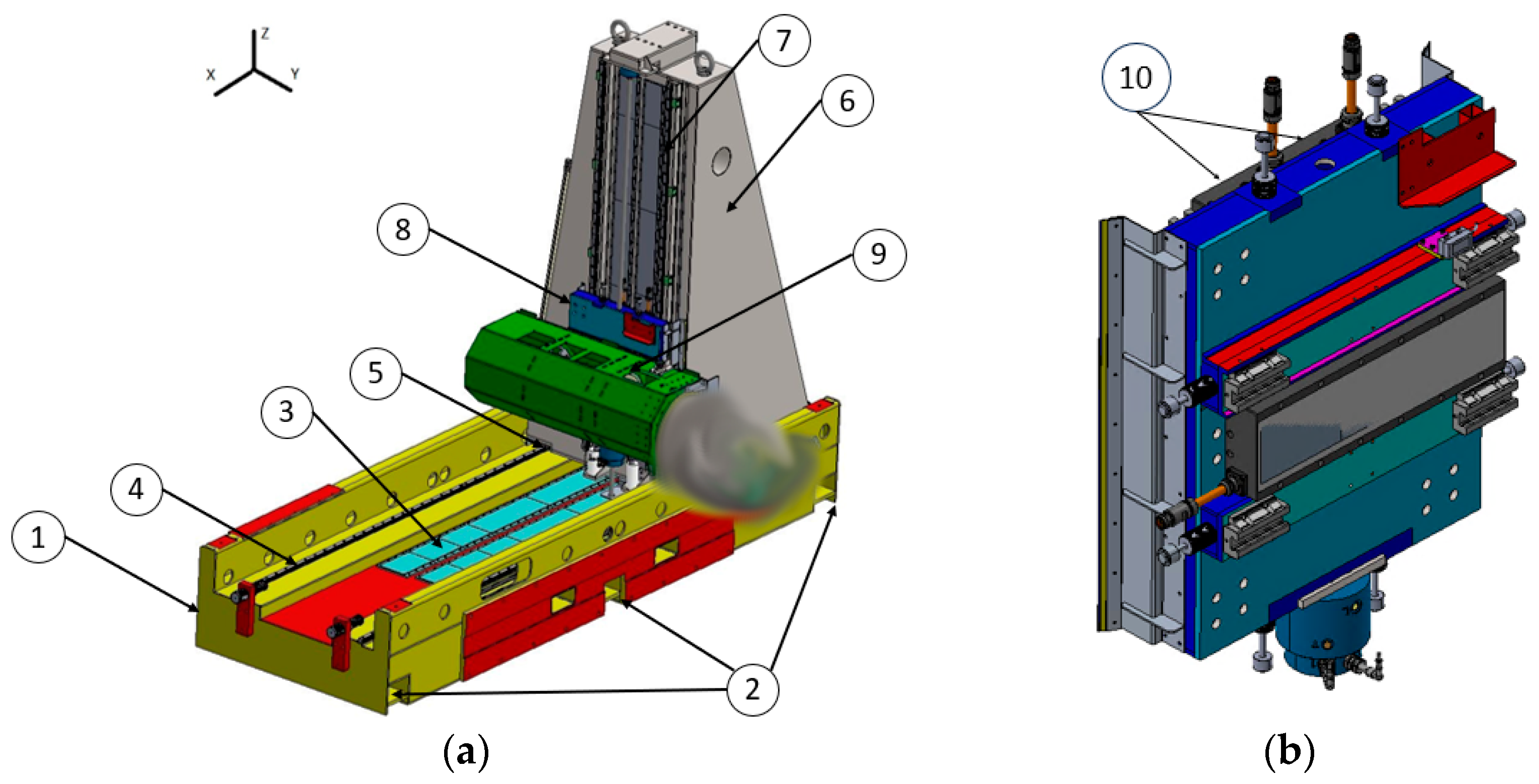
2. Cartesian Robot Description

The Cartesian robot prototype object of the present paper was designed to perform rapid movement for metal sheet cutting in the automotive field. A CAD model is reported in Figure 1a. Part of the robot is blurred since design confidentiality applies. Nonetheless, the robot can be split into a “host machine” and a “head”. The “host machine” is a Cartesian robot that translated the “head”, i.e., blurred part, in the cartesian working volume.

From a system point of view, the robot is composed of a welded steel basement (1) that on one hand allows for the connection to the ground by means of M20 bolts (2), and on the other hand, it provides adequate space for the placement of magnetic plates (3) and tracks (4). Six linear bearings (5) and electric motors are jointed under the column (6). The shape coupling between the slides (5) and the tracks (4) allows for an accurate and rigid guiding system. The magnetic interaction between the motors and the plates (3) provides the necessary force along the X axis. By exploiting the same linear actuation principles, i.e., the magnetic interaction between two linear electric motors (10) and the magnetic plates (7) fixed on the column, the Z Carriage (8), reported also in Figure 1b, allows for the translation along the Z axis. Additionally, the Z Carriage bears the weight of the motors that ensure the motion both on the Z direction and on the Y direction. Furthermore, the Z Carriage sustains loads and dynamic actions generated by the AY group (9). The Z Carriage, made of welded steel, ribs, and stiffeners, is, therefore, a critical component as it performs multiple functions, and its footprint must be limited to allow for a reduced stroke along the Z and Y directions. For these reasons, the aim of the study will be to find out an optimal material distribution able to maximize the Z Carriage stiffness, by keeping the current overall dimensions as design volume boundaries.

3. Methodology

3.1. Static Optimization Problem

An optimization process generally foresees the minimization or maximization of some design objectives, by acting on some design variables and respecting some equality or inequality constraints. In the case of topology optimization, different design objectives can be defined as well as constraints [16], depending on the specific needs and design requirements. For the purpose of the present work, the Topology Optimization (TO) problem can be formulated as the optimal material distribution that can minimize the global compliance of the specific structure, by respecting fractional mass and static load constraints. Formally, the mathematical problem can be formulated according to Equations (1)–(4).

The formulation of the compliance arises from the pioneering work presented in [17], and it is also employed in the commercial code MSC Nastran [18] used for the specific analysis. TO generally involves a very large number of design variables, because it is coincident with the number of elements of a component mesh. Furthermore, the objective is to understand if, for the specific boundary condition, an element in the design volume is essential and must be kept (a “1” value is then assigned) or it is useless and can be eliminated (a “0” value is assigned). The Solid Isotropic Microstructure with Penalization (SIMP) method [19] is one of the most employed methods in the literature and represents a great advantage in terms of robustness and simplicity because it redirects a large problem to an equivalent “thickness optimization” one [20] in which only the density parameters play a key role. Furthermore, it allows to overcome the fact that TO problems are ill-posed since they tend to generate designs with a large number of microscopic holes, rather than a low number of macroscopic holes [18]. The solution is made possible thanks to the use of mesh-independent filtering techniques, first proposed by Sigmund [21]. The basic idea stood in the use of a linear low-pass convolution procedure which could allow to pass from the checkerboard-optimized design (only 0/1 regions) to the generation of intermediate grey areas. The filter application then allows for a continuous density variation in the design, i.e., from 0 to 1. The advantage is that possible local minima are not a priori disregarded by the optimizer, the Method of Feasible Direction can be applied, and fewer design variables are involved. Once the optimized solution is reached, grey areas may be present. The additional feature of the method is the penalty factor, p, that, by means of an exponential law, diminishes the contribution of grey elements to the total stiffness and allows for a clear distinction between the elements to keep (1) and elements to disregard (0). Generally, a value between 3 and 5 is used.

As anticipated, the problem is mathematically formulated according to the following:

Min

$$H_{gl}\left(\mathit{x}\right)={\mathit{U}}^T{\mathit{K}}_{\mathit{g}\mathit{l}}\mathit{U}=\sum _{e=1}^N{\mathit{x}}_e^p{\mathit{u}}_e^T{\mathit{K}}_e^0{\mathit{u}}_e$$

(1)

Such that:

$${\mathit{K}}_{\mathit{g}\mathit{l}}\left(\mathit{x}\right)\mathit{u}=\mathit{F}$$

(2)

$$\frac{\sum _{e=1}^N{\mathit{x}}_e{\mathit{V}}_e}{V}\le {FRMASS}_{UB}$$

(3)

$$0\le {\mathit{x}}_e\le 1$$

(4)

where:

• $H_{gl}$ is the global compliance of the structure and indicated how much the structure deforms when a force is applied: it can also be defined as twice the strain energy;
• $\mathit{U}$ is the global displacement vector of the structure nodes;
• ${\mathit{K}}_{\mathit{g}\mathit{l}}$ is the global stiffness matrix of the structure;
• ${\mathit{x}}_e$ is the design variable vector;
• $p$ is the penalty factor;
• ${\mathit{u}}_e$ is the element displacement vector;
• ${\mathit{K}}_e^0$ is the elemental stiffness matrix;
• $\mathit{F}$ is the external load vector for which the optimization is necessary;
• ${\mathit{V}}_e$ is the volume of the element;
• $V$ is the total design volume;
• ${FRMASS}_{UB}$ is the upper bound allowed for the fractional mass, strictly connected to the design purposes.

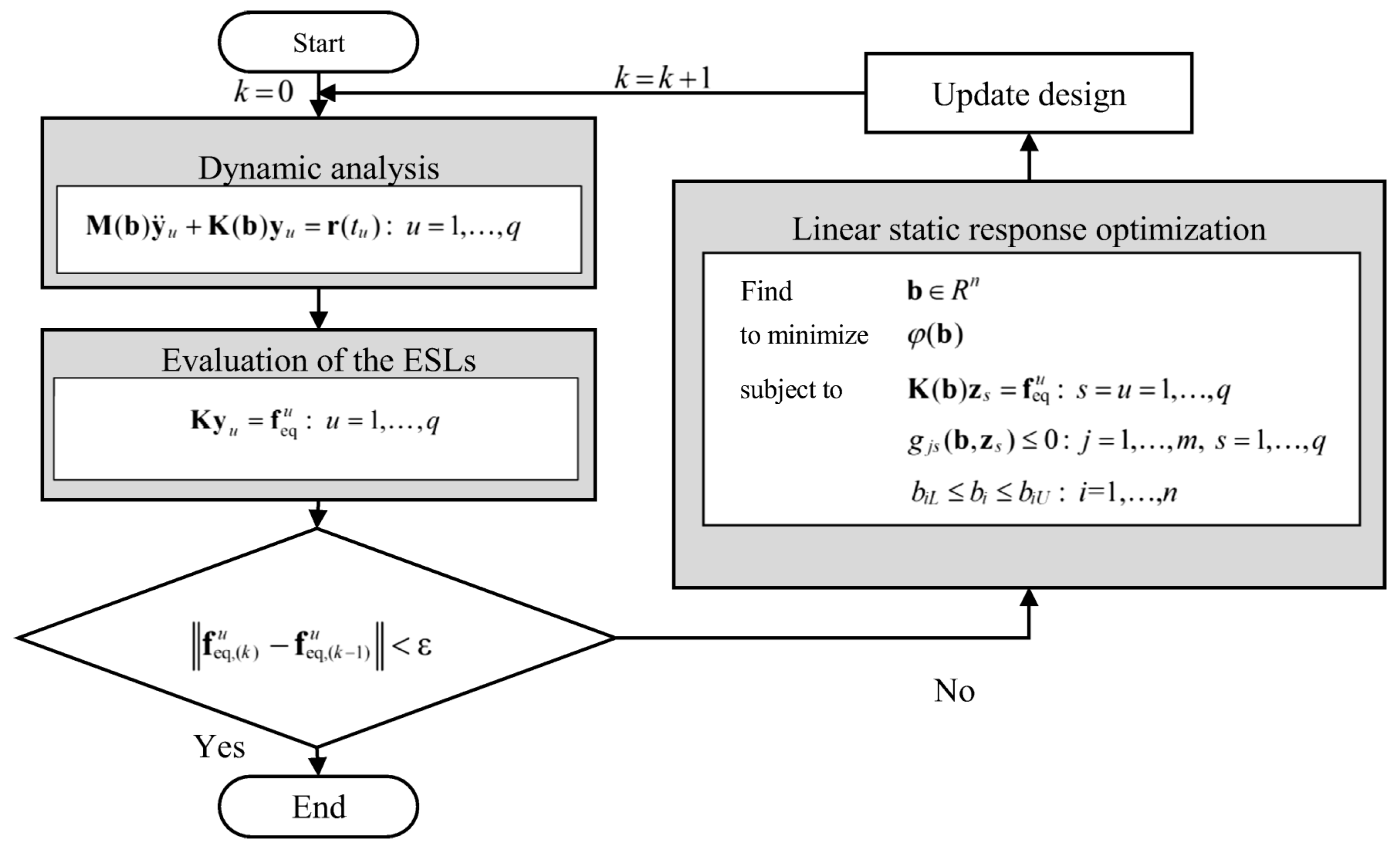
3.2. Equivalent Static Loads Method

3.2.1. ESL in the Literature

The idea behind the ESL method is quite simple. In general, for a dynamic problem, the equation of motion of a linear, M-DoF, damped system undergoing a forced response can be written according to Equation (5). The same equation holds also in the case of an FE model undergoing a time-dependent load and for which a material and damping model is applied.

$$\mathit{M}\ddot{\mathit{x}}\left(t\right)+\mathit{C}\dot{\mathit{x}}\left(t\right)+\mathit{K}\mathit{x}\left(t\right)=\mathit{F}\left(t\right)$$

(5)

where:

• $\mathit{M}$ is the mass matrix;
• $\mathit{C}$ is the damping matrix;
• $\mathit{K}$ is the stiffness matrix;
• $\mathit{x}\left(t\right),\dot{\mathit{x}}\left(t\right),\ddot{\mathit{x}}\left(t\right)$ is the displacement vector and its first and second time derivatives, respectively;
• $\mathit{F}\left(t\right)$ is the load vector that generally contains many null elements.

Equation (5) can also be rewritten according to the following:

$$\mathit{K}\mathit{x}\left(t\right)=\mathit{F}\left(t\right)-\mathit{M}\ddot{\mathit{x}}\left(t\right)-\mathit{C}\dot{\mathit{x}}\left(t\right)$$

(6)

The equilibrium equation for a static problem is instead identified by:

$$\mathit{K}\mathit{x}=\mathit{E}\mathit{S}\mathit{L}$$

(7)

where $\mathit{E}\mathit{S}\mathit{L}$ is a static load vector.

The relation between Equations (6) and (7) indicates that if the displacement vector and its relative derivatives from Equation (6) are known for each time step, it is possible to reconstruct a static displacement field which is equivalent to the dynamic one for each time step. The static displacement field can therefore be reproduced, for each time step, by a set of static loads defined as Equivalent Static Loads (ESLs). The ESLs can therefore be computed, for each time step, according to Equation (8).

$$\mathit{E}\mathit{S}\mathit{L}\left(t\right)=\mathit{K}\mathit{s}\left(t\right)$$

(8)

where $\mathit{s}\left(t\right)$ is the computed solution to the dynamic problem of Equation (5).

From a practical point of view, it is then necessary to perform a transient analysis to first obtain the displacement vector $\mathit{s}\left(t\right)$ necessary to compute the ESL. Secondly, a criterion is needed to understand at which time step the ESL could actually be relevant for the optimization purposes. Thirdly, the original load vector F(t) is generally characterized by few non-null elements, as in standard practice the forces applied to an element can be modelled by using few master nodes, whilst in this case the ESL should be applied to each node of the structure or, in the best-case scenario, an approximation must be introduced by neglecting the less relevant ESL according to some case-dependent criterion. To provide the complete picture, the ESL method generally follows an iterative procedure, as indicated in Figure 2 [15]. As previously mentioned, different criteria could be used to build the objective function. As for the application points, no indication is reported in the literature on how to simplify the problem, which could be quite demanding when dealing with FE model set-up.

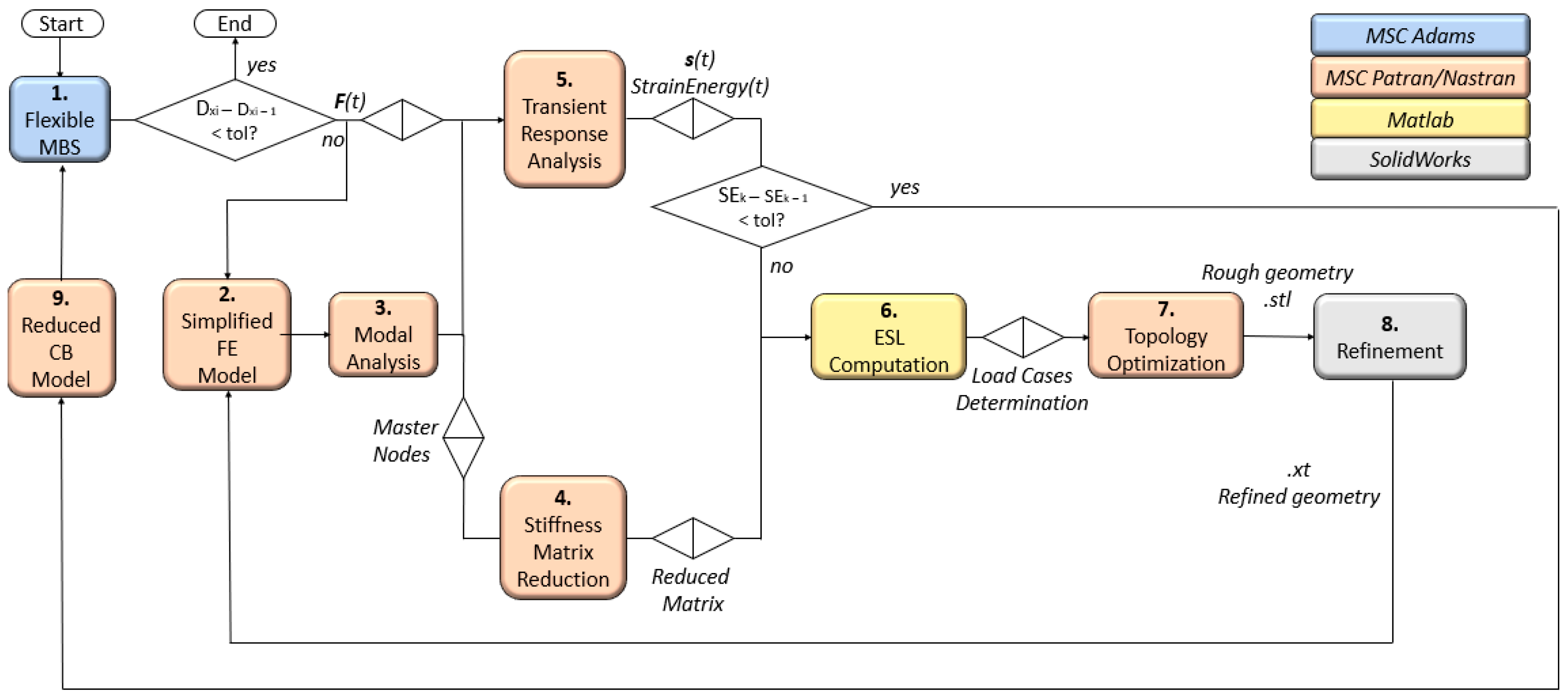
3.2.2. ESL in the Present Work

The aim of the methodology hereby presented is to introduce the reader to the process, choices, and software programs adopted to perform the structural optimization of a flexible mechanism component based on a modified ESL method. The objective is the reduction in the Tool Center Point (TCP) trajectory deviations of the abovementioned robot. The deviations for the reference and “optimized” cases were evaluated by means of flexible multibody simulations.

The methodology illustrated in Figure 3 consists in the following points:

• the flexible MultiBody Simulation (MBS) is the first necessary step in order to obtain the forces exchanged at the boundary nodes and to assess how the structure flexibility affects the spatial deviation of the TCP from the nominal trajectory. The flexible MBS is the first step of the external analysis and verification cycle.
• A simplified FE model that reproduces the inertial and stiffness properties of specific sub-assembly is created. The simplified FE model contains the real geometry of the component to be optimized (i.e., Z Carriage). The simplified model creation (or updating) represents the first step of the internal optimization cycle.
• An initial modal analysis is suggested to identify the relevant modes for the specific analysis and to understand which are the maximum relative displacement nodes. The maximum relevant displacement nodes for the modes of interest represent the master nodes to use for the Guyan reduction.
• The reduced stiffness matrix related to the specified master nodes is obtained by means of a Guyan reduction.
• The dynamic forces computed in the multibody model are provided as input for the transient analysis in the internal optimization cycle. The important outputs of the transient analysis are both the global strain energy over time and the displacements of the master nodes.
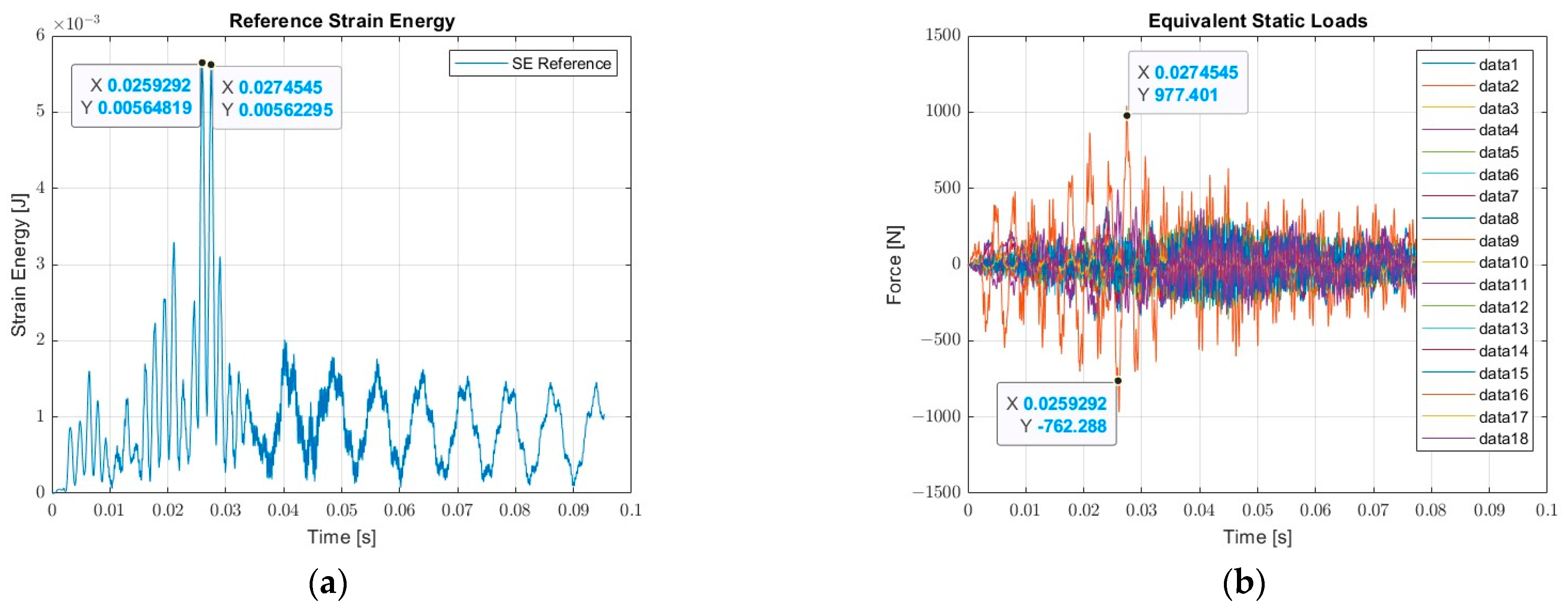
• The reduced stiffness matrix and the displacements of the master nodes along three directions are multiplied to obtain the ESL matrix. The matrix represents the ESL for each time step of the simulation. The time instants corresponding to the strain energy peaks are the discriminant parameter for the selection of the most relevant ESL. The main output of this phase is a set of load cases to be applied to the master nodes for the optimization. The number of load cases depends on the strain energy peaks number.
• Once the design volume of the component is specified, the optimization is run. The objective is to find the mass distribution in the available design volume that minimizes the global compliance of the structure, by imposing a constraint on the mass fraction, evaluated according to Equation (3). The value of the upper bound, i.e., ${FRMASS}_{UB}$ in Equation (3), was selected to guarantee the same mass values between the original design and the optimized one.
• The optimization output is then manually post-processed to create a smooth CAD version of the optimized component, i.e., the refinement process. The internal optimization cycle is then repeated (back to 2) until the strain energy peaks minimization is obtained. The output of the cycle is the geometry and, consequently, the mesh of the optimized component.
• The flexible multibody model is updated with the new geometry (a Craig–Bampton reduction is performed), and a new analysis is carried out. For the sake of the optimization procedure, if the TCP accuracy increases, the geometry can be considered feasible, pending manufacturability verification.

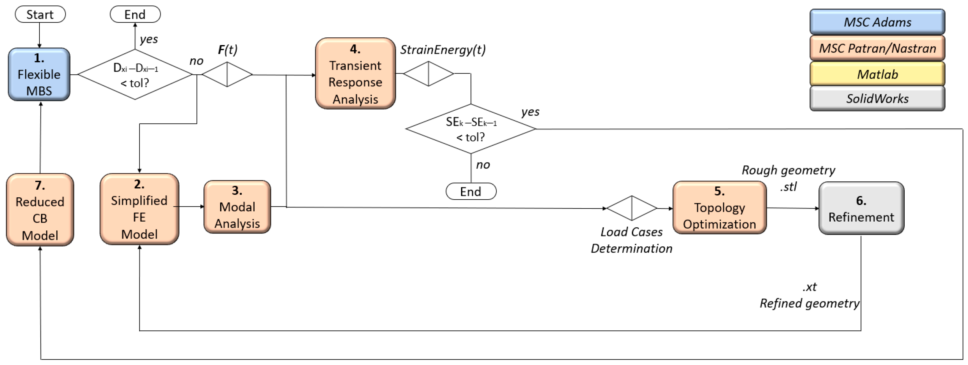
3.3. Quasi-Static Loads method

The Quasi-Static Loads (QSL) method is similar to the previous one for many operations involved, as shown in Figure 4, in fact:

• A flexible MBS allows for the determination of dynamic loads.
• A simplified FE model reproduces the sub-assembly characteristics.
• A modal analysis is performed to determine the modal characteristics of the structure.
• A transient response analysis is performed to determine the strain energy of the structure before and after optimization.
• The topology optimization is performed, but there are few load cases and the loads are applied only on the boundary nodes (this is not necessarily true in the case of the ESL method).
• A refinement step is carried out after topology optimization to obtain a smooth geometry.
• A reduced CB model is implemented to verify the new geometry, and a final multibody verification is carried out.

The main difference lies in the fact that the ESL computation as well as the static reduction are no longer required. Furthermore, the internal and external cycles are only performed once because no minimization operation of the peak strain energy is involved. As a result, it is much faster with respect to the ESL one. The point is then to understand whether the ESL methodology can actually provide an added value to the optimization process or, if for the specific purposes, the QSL methodology is sufficient.

4. QSL Method and ESL Method Comparison

4.1. Simple Case—Beam

The comparison of the two methods was first carried out on a simple, reproducible case, a hollow beam. The purpose is first to validate the internal cycle (Figure 3) and, secondly, to evaluate the advantages of the ESL method with respect to the QSL one. The chosen reference model is representative of the real component (Z Carriage) because the beam is characterized by a hollow cross section, and the multiaxial loads are applied on two different nodes. Moreover, the loads applied on the different nodes also have a phase difference of 90°.

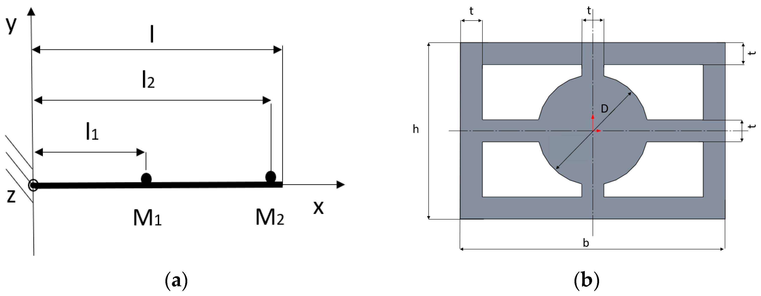
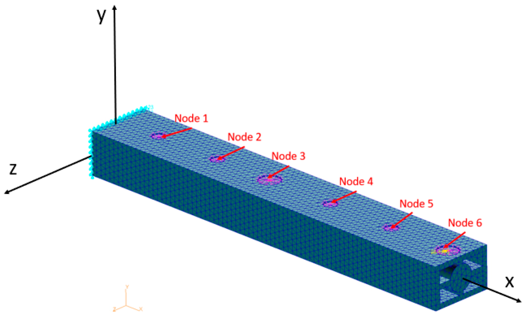
4.1.1. Cantilever Beam Geometry

In Figure 5, a schematic representation of the beam is depicted. In

Table 1. Mechanical system parameters.

Parameter	Value
D [mm]	50
b [mm]	120
h [mm]	80
t [mm]	10
l1 [mm]	350
l2 [mm]	760
l [mm]	780
M1 [kg]	24
M2 [kg]	15

and

Table 2. Beam material mechanical properties.

Parameter	Value
E [GPa]	70
ν [-]	0.3
ρ [kg/m3]	2700

, the geometric and mechanical parameters are listed.

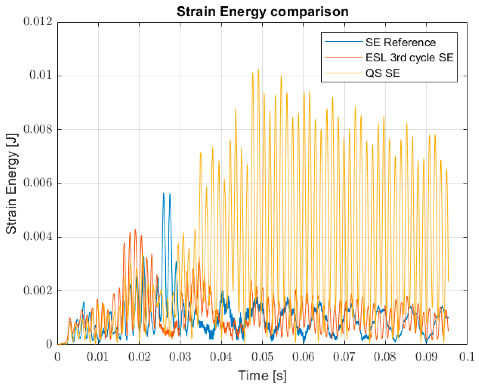
4.1.2. Transient Analysis Set-Up

Figure 6 shows the picture of the meshed beam. The system was modelled by using tetrahedral elements of the 1st order, additional masses modelled as concentrated ones and connected to RBE2 elements, in correspondence of Node 3 and Node 6. The six nodes reported in the figure were also used as master nodes for the static reduction. The beam was constrained on one end, and two force vectors were applied in Node 3 and Node 6. The force applied in Node 6 is random multiaxial. The actual trends over time for the Y and Z directions are reported in Figure 7. No force was applied along the X direction. The force applied in Node 3 is five times higher than the previous one in Node 6 and shifted by 90°.

The output of the dynamic analysis is reported in Figure 8a, whilst in Figure 8b, the computed ESLs are depicted. The time instants corresponding to the maximum values of the strain energy were selected as key time instants for the definition of the load cases in the case of optimization following the ESL approach. As can be noticed, the maximum values of the ESL do not necessarily represent the worst case in terms of applied deformation energy. The strain energy peaks selection for the definition of the ESL load cases is therefore more reliable.

For the QSL method instead, the load cases are selected by taking into account just the two nodes in which the loads are actually applied. Furthermore, only the maximum force values are considered since the dynamic effects of the structure are neglected. It generates reduced load cases for the topology optimization set-up, and it requires fewer operations for the boundary conditions definition.

As can be realized, there are major differences between the ESL and QSL methods. The computation of the ESL foresees the use of the transient analysis output as input (Equation (5)). The transient response, therefore, generates a complex load condition on “several” nodes since resonant frequencies may be excited in different directions due to the load frequency content, thus inducing global strain energy peaks in some specific time instants. The global strain energy peaks depend then on the modal characteristics of the structure (eigenvectors and eigenfrequencies) and on the frequency content of the load applied. The boundary conditions for the optimization, therefore, take into account the actual critical time instants (peaks of the strain energy) and a more accurate spatial distribution of the dynamic loads (selection of “smart” master nodes, i.e., Nodes 1–6).

The QSL method, by definition, does not consider the time-varying nature of the load applied, thus using as optimization boundary conditions just the envelope values of the loads applied (maximum and minimum values in Figure 7) in the specific boundary nodes (Node 3 and Node 6).

The response of the structure is thus disregarded both in terms of spatial and time domains, thus introducing a strong approximation.

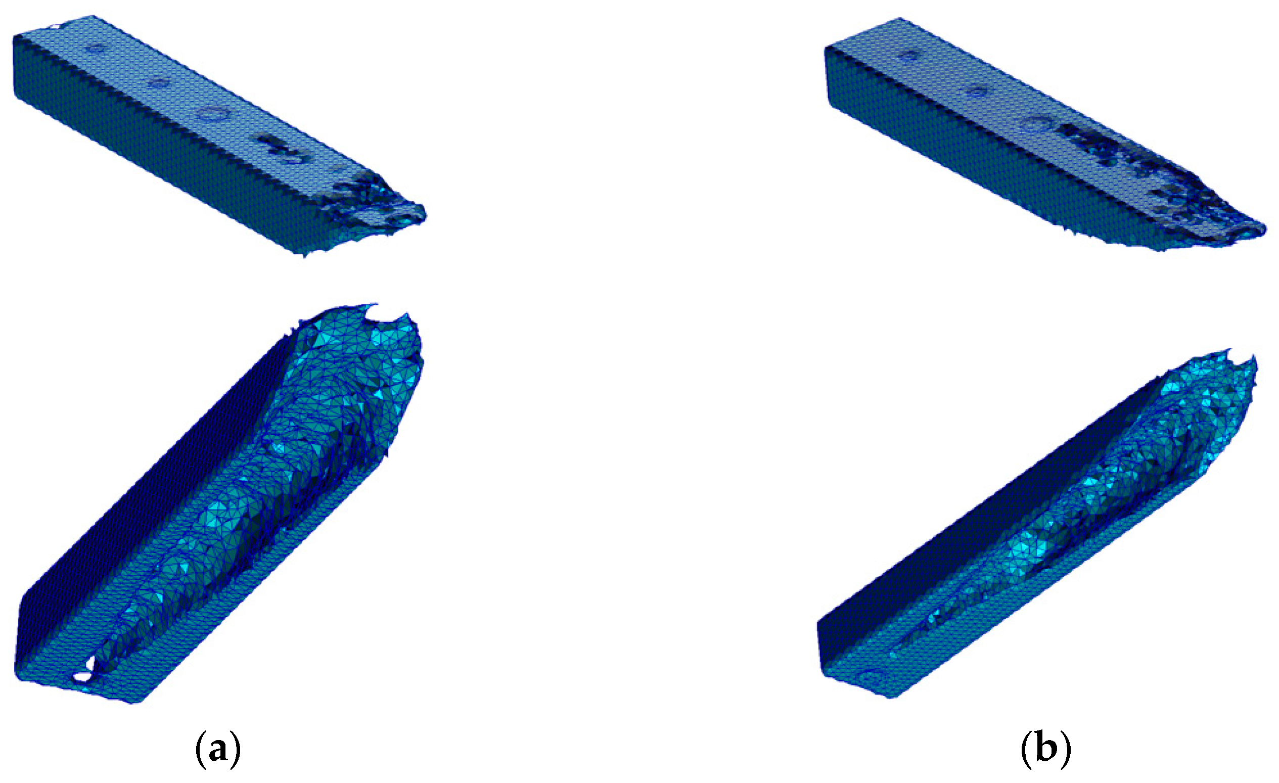
4.1.3. Optimization Output Comparison

In Figure 9, the topology optimization outputs are reported. The two designs apparently share similar mass distribution, as both distribute the mass in correspondence of the external part. This choice is reasonable from a theoretical point of view since the beam is loaded by bending loads and the mass concentration in correspondence of the external region maximized the inertia bending moments. Nonetheless, the ESL method foresees a more symmetrical design with respect to the QSL method. The lack of symmetry may be connected to the fact that no manufacturing constraint was imposed for the analysis and that the load sets are either complex as in the case of the ESL method or strongly directional as in the case of the QSL method. Furthermore, in Figure 10, the strain energies obtained after the transient analysis of the refined geometries demonstrate a clear winner between the two methods. As can be evidenced, the mass distribution foreseen by the QSL optimization leads to a strain energy maximum increase close to twice the reference condition, even though up to 0.3 s, the results are comparable. Probably, the different mass distribution leads to different modal participation factors that amplify the response of the structure, once enough energy is input into the system.

The ESL method instead leads to a strain energy maximum reduction of roughly 30%. As indicated in

Table 3. ESL method and QS method comparison.

Parameter	Reference	ESL Cycle 3	QSL
Weight [kg]	13.1	13.2	13.2
1st Bending XY [Hz]	47.4	50.7	51.0
1st Bending XZ [Hz]	66.4	81.3	81.6
2nd Bending XY [Hz]	249	240	224
1st Torsion X [Hz]	318	369	360
Node 6 Δxmax [m]	1.23 × 10−6	1.57 × 10−6	1.94 × 10−6
Node 6 Δymax [m]	5.94 × 10−6	1.07 × 10−5	4.88 × 10−6
Node 6 Δzmax [m]	5.30 × 10−5	2.03 × 10−5	5.88 × 10−5
Peak SE [J]	5.65 × 10−3	4.30 × 10−3	1.02 × 10−2

, a clear advantage is obtained also in terms of maximum displacement reduction in correspondence of Node 6. The natural frequencies of the optimized geometries always increase with respect to the reference condition, with the exception of the 2nd Bending XY of the QSL method.

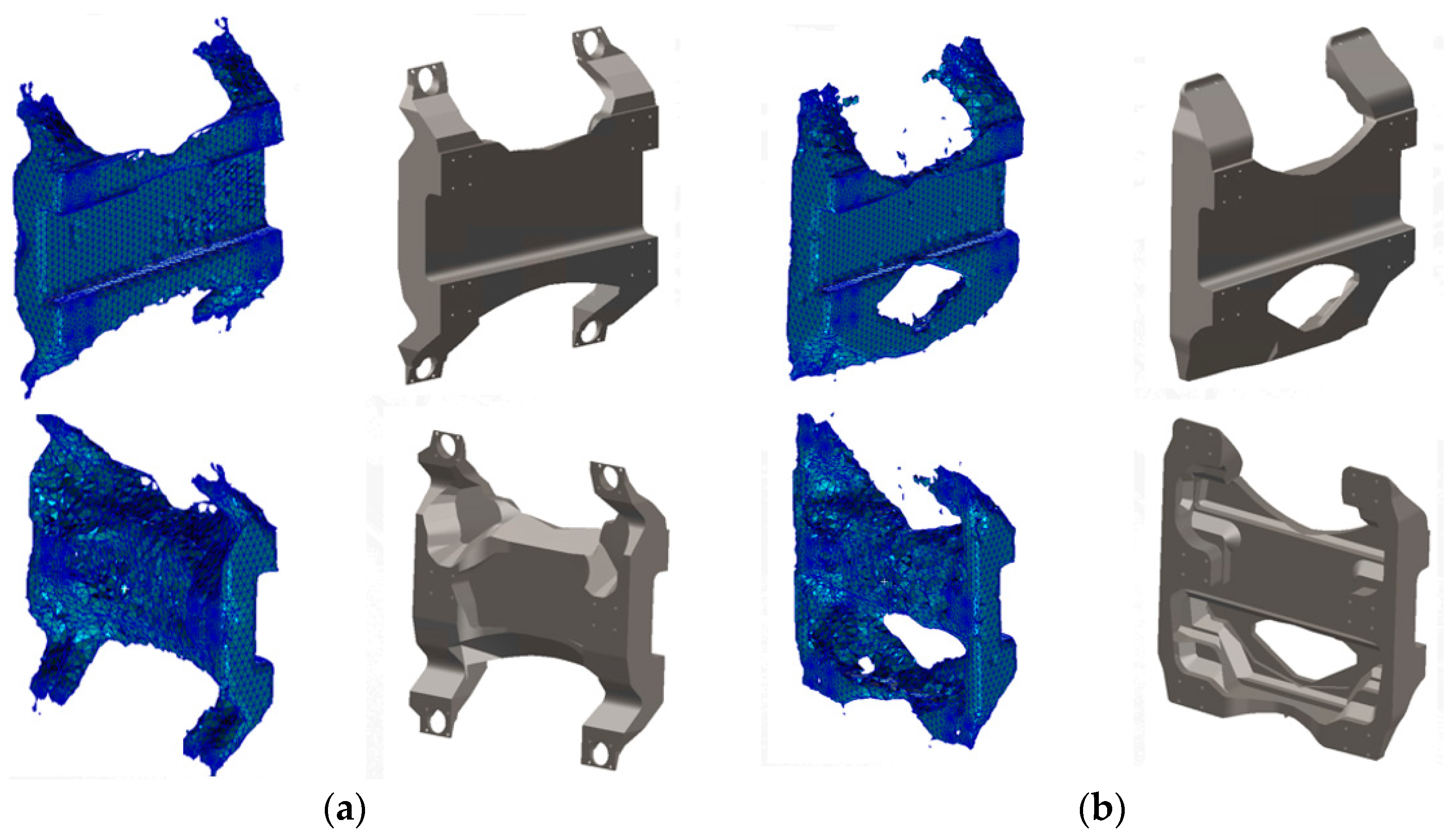
4.2. Real Case—Z Carriage

For the Z Carriage optimization, a flexible multibody simulation was run to identify which were the loads acting on the interface points of the component (Figure 11). The flexible multibody model was tuned to experimental data previously obtained. The axis movement was implemented by splines reproducing the exact coordinated movement of the machine axes. Therefore, the frequency content of the force exchanged in correspondence of the Interface Points (IP) had the frequency content experienced by the real components. According to the multibody model and real machine, the AY group (shown in Figure 1) exchanged forces by means of slides, and consequently screws, in correspondence of the selected IP.

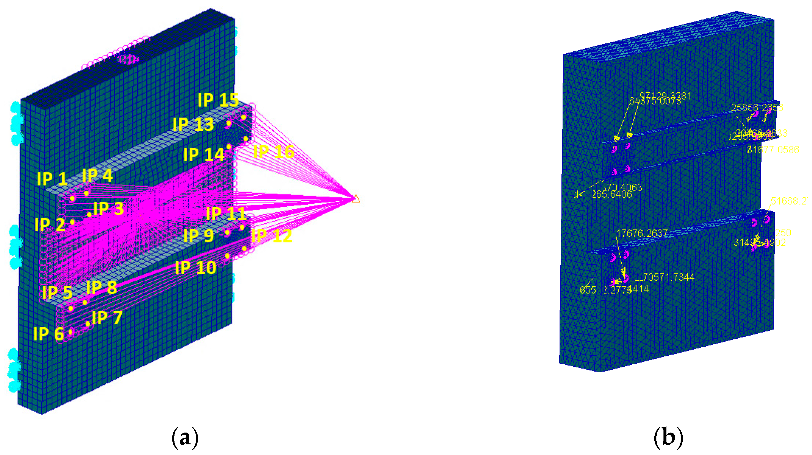
4.2.1. Finite Element Model

Once the loads were derived, an additional simplification was necessary in order to perform the transient analysis. Basically, a simplified FE model of the sub-assembly Z Carriage and AY group was created. The “stiff” elements, such as motors, brakes, and AY group, were modelled as point masses and inertias (CONM2) at the corresponding centers of mass connected to the Z Carriage, modelled as surfaces with quadrilateral mesh (CQUAD4 elements), by means of RBE2. The idea of these modelling choices was to reproduce, as faithfully as possible, the modal characteristics of the sub-assembly. The simplified model presented, overall, 4640 elements and 18,202 nodes. Given the type of surface element that presents 6 Degrees of Freedom (DOFs), a total number of 109,212 DoFs were taken into account during the analysis. The thickness information was provided by means of properties assignment, through the PSHELL function.

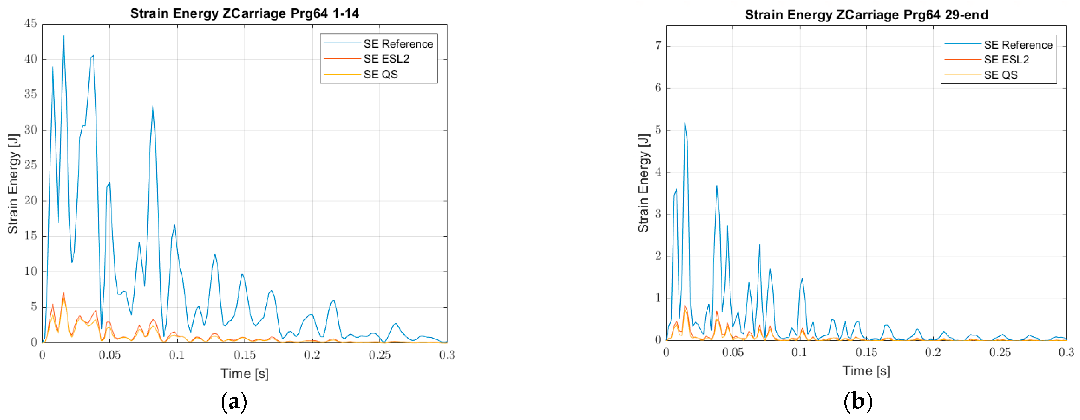
4.2.2. Topology Optimization Output Comparison

As for the analysis, with an available physical memory of 23,410 MB, available paging file size of 25,968 MB, and a virtual memory available of 13.4 TB, for the ESL, the optimization lasted for 315 s, and the final result was obtained at the 19th design cycle. In the case of QSL, with the same available resources, the optimization was reached after 31 cycles and in 1230 s. If, on the one hand, the optimization time is greatly reduced in the case of ESL, it must be borne in mind that the set-up time for the additional operations (i.e., static reduction and ESL computation) plays an opposite role. The overall time comparison may provide an interesting information if the overall procedure is considered, but to be significant, both procedures presented in Figure 3 and Figure 4 should be automatized. This is not the case yet as many operations were performed manually and the aim of the comparison in this stage was to compare the effectiveness of one method with respect to another in terms of components stiffness (strain energy), rather than methods efficiency.

In Figure 12, the topology optimization outputs and relative refinements of the two methods are reported. The two geometries show different mass distributions, even though both of them suggest a mass distribution reduction in the central zones. The result is reasonable since the applied forces are close to the constraints. With the applied forces being close to the constraint on both sides, these zones will experience the highest deformation, whilst the central zones will be less involved. Basically, the load path will pass through the central zones in a negligible way. The optimization outputs are symmetrical, as in this case, the symmetry manufacturing constraint was imposed for the optimization. Furthermore, both outputs presented limited zones in which disjointed fibers are present. This, of course, is not likely in reality; therefore, during the refinement process, the disjointed fibers were eliminated since they accounted for a negligible amount.

In order to highlight the differences between the two methods, the following computations were performed on the two updated geometries.

(1)

Transient analysis to calculate the strain energies at the most critical trajectories, some relevant time intervals are shown in Figure 13.

(2)

Flexible multibody simulation to calculate the maximum deviations from the nominal trajectories of the two models, as shown in

Table 4. Flexible multibody simulation outputs comparison for Z Carriage.

Trajectory	Deviation	Reference	ESL Cycle 2	QSL
Trajectory 1	Δx [m]	0.025700	−16.30%	−17.69%
	Δy [m]	0.007159	−23.72%	−26.46%
	Δz [m]	0.012687	−15.75%	−16.02%
Trajectory 2	Δx [m]	0.002871	−16.91%	−18.47%
	Δy [m]	0.001037	−12.41%	−13.52%
	Δz [m]	0.001086	−12.68%	−13.72%
Trajectory 3	Δx [m]	0.002498	−17.15%	−19.12%
	Δy [m]	0.000896	−14.84%	−16.81%
	Δz [m]	0.00077	−15.68%	−16.47%
Trajectory 4	Δx [m]	0.001898	−17.35%	−17.88%
	Δy [m]	0.000789	−8.92%	−8.56%
	Δz [m]	0.003128	−18.53%	−15.25%

.

As can be appreciated in Figure 13, both methods lead to a remarkable decrease in terms of strain energy, meaning that the overall deflection of the Z Carriage is reduced if compared to the initial design. In detail, the QSL method seems to perform slightly better even if no relevant difference is present between the two methods. This may be justified by the fact that the frequency content values of the loads applied to the Z Carriage are relevant up to 50 Hz, whilst the first natural frequency of the Z Carriage and YY Group (Figure 11a) is 407 Hz.

This shows that, in general, the frequency ratio between the load band and the first natural frequency of the sub-system must be taken into account before performing a topology optimization. If the frequency ratio is, as in this case, about 0.15, an optimization according to a Quasi-Static approach shall be preferred.

Similar conclusions can be reached by analyzing the deviations from the robot cutting tool desired trajectory. The optimization process should lead to a decrease in the deviation from the desired trajectory. Table 4 lists the percentage variation of the deviation values. It can be observed that both methods lead to a percentage reduction in the deviation, that is, a reduction in the error with respect to the reference trajectory, for different types of trajectories. This reduction is due to the fact that the system is stiffer overall. The reductions are of the same order of magnitude for the two methods, with slightly higher reduction values for QS.

5. Conclusions

The paper presents an optimization procedure based on the ESL method with an intermediate static Guyan reduction to properly select the loads application point and reduce the FE model set-up time. A comparison between the ESL method and the QSL method is performed both for a simple test case and for a real component of a Cartesian robot. The ESL method can represent a smart strategy to take into account the modal properties of a component/structure, thus avoiding a topology optimization in a dynamic field; nonetheless, for practical cases, the QSL approach can still be valid to obtain remarkable results.

Consequently, the subsequent computational steps outlined below offer practical guidelines for approaching the topology optimization of flexible mechanisms.

-

A system-level flexible multibody analysis to assess the dynamic behavior of the structure.

-

A preliminary sensitivity analysis to understand how much the individual component contributes to the overall stiffness of the system. The preliminary analysis should also study the feasibility of the redesign based on the requirements and design phase.

-

Modal analysis (before optimization) using the FE model of the subset in which the component to be optimized is present. The advantage of this preliminary modal analysis is twofold: computation of natural frequencies and identification of the nodes with the largest relative displacement to be identified.

-

Analysis of the frequency content of the loads applied to the component, before performing the optimization. The ratio between the maximum relevant frequency of the force and the first natural frequency of the component gives an indication for the optimization method selection. The QSL method should be preferred for a frequency ratio about or below 0.15.

-

An intermediate Guyan static condensation is suggested when applying the ESL method. The selection of few “smart” nodes allows for the reduction in computation time for the optimization, increasing as well the design volume available for the process.

-

Evaluation of the ESL at the time instants of the strain energy peaks rather than blindly selecting the absolute maximum values of the ESL, for the boundary conditions of the optimization process. It is, in fact, not always guaranteed that the highest forces, if applied in few nodes, represent appropriate boundary conditions for the optimization.

References

1. Tromme, E.; Held, A.; Duysinx, P.; Brüls, O. System-Based Approaches for Structural Optimization of Flexible Mechanisms. Arch. Comput. Methods Eng. 2018, 25, 817–844. [Google Scholar] [CrossRef]
2. Min, S.; Kikuchi, N.; Park, Y.C.; Kim, S.; Chang, S. Optimal Topology Design of Structures under Dynamic Loads; Springer: Berlin/Heidelberg, Germany, 1999. [Google Scholar]
3. Rong, J.H.; Xie, Y.M.; Yang, X.Y.; Liang, Q.Q. Topology optimization of structures under dynamic response constraints. J. Sound Vib. 2000, 234, 177–189. [Google Scholar] [CrossRef]
4. James, K.A.; Waisman, H. Topology optimization of viscoelastic structures using a time-dependent adjoint method. Comput. Methods Appl. Mech. Eng. 2015, 285, 166–187. [Google Scholar] [CrossRef]
5. Vanpaemel, S.; Asrih, K.; Vermaut, M.; Naets, F. Topology optimization for dynamic flexible multibody systems using the Flexible Natural Coordinates Formulation. Mech. Mach. Theory 2023, 185, 105344. [Google Scholar] [CrossRef]
6. Albers, A. Automated Topology Optimization of Flexible Components in Hybrid Finite Element Multibody Systems Using ADAMS/Flex and MSC. Construct. Available online: https://www.researchgate.net/publication/36452967 (accessed on 18 June 2023).
7. Albers, A.; Ottnad, J.; Häußler, P.; Minx, J. Structural Optimization of Components in Controlled Mechanical Systems. 2007. Available online: http://www.asme.org/about-asme/terms-of-use (accessed on 18 June 2023).
8. Institute of Electrical and Electronics Engineers; IEEE Robotics and Automation Society. Humanoids ’09: [proceedings]. In Proceedings of the 9th IEEE-RAS International Conference on Humanoid Robots, Paris, France, 7–10 December 2009. [Google Scholar]
9. Kang, B.S.; Choi, W.S.; Park, G.J. Structural Optimization under Equivalent Static Loads Transformed from Dynamic Loads Based on Displacement. Available online: www.elsevier.com/locate/compstruc (accessed on 4 July 2023).
10. Choi, W.S.; Park, G.J. Structural Optimization Using Equivalent Static Loads at All Time Intervals. Available online: www.elsevier.com/locate/cma (accessed on 4 July 2023).
11. Park, G.J.; Kang, B.S.; Choi, K.K. Technical Note Validation of a Structural Optimization Algorithm Transforming Dynamic Loads into Equivalent Static Loads 1. J. Optim. Theory Appl. 2003, 118, 191–200. [Google Scholar] [CrossRef]
12. Jang, H.H.; Lee, H.A.; Lee, J.Y.; Park, G.J. Dynamic response topology optimization in the time domain using equivalent static loads. AIAA J. 2012, 50, 226–234. [Google Scholar] [CrossRef]
13. Stolpe, M. On the equivalent static loads approach for dynamic response structural optimization. Struct. Multidiscip. Optim. 2014, 50, 921–926. [Google Scholar] [CrossRef]
14. Stolpe, M.; Verbart, A.; Rojas-Labanda, S. The equivalent static loads method for structural optimization does not in general generate optimal designs. Struct. Multidiscip. Optim. 2018, 58, 139–154. [Google Scholar] [CrossRef]
15. Park, G.J.; Lee, Y. Discussion on the optimality condition of the equivalent static loads method for linear dynamic response structural optimization. Struct. Multidiscip. Optim. 2019, 59, 311–316. [Google Scholar] [CrossRef]
16. Olhoff, N.; Taylor, J.E. On Structural Optimization. 1983. Available online: http://asmedigitalcollection.asme.org/appliedmechanics/article-pdf/50/4b/1139/6362856/1139_1.pdf (accessed on 12 January 2023).
17. Bendse, M.P.; Kikuchi, N. Generating Optimal Topologies in Structural Design Using a Homogenization Method. Comput. Methods Appl. Mech. Eng. 1988, 71, 197–224. [Google Scholar] [CrossRef]
18. MSC Nastran 2022.2 Design Sensitivity and Optimization User’s Guide MSC Nastran Design Sensitivity and Optimization User’s Guide. 1992. Available online: http://msc-documentation.questionpro.com (accessed on 15 February 2023).
19. Rozvany, G.I.N. A critical review of established methods of structural topology optimization. Struct. Multidiscip. Optim. 2009, 37, 217–237. [Google Scholar] [CrossRef]
20. Rozvany, G.I.N. The Simp Method in Topology Optimization-Theoretical Background, Advantages and New Applications. In Proceedings of the 8th Symposium on Multidisciplinary Analysis and Optimization, Long Beach, CA, USA, 6–8 September 2000. [Google Scholar]
21. Sigmund, O. Design of Material Structures using Topology Optimization. Ph.D. Thesis, Technical University of Denmark (DTU), Lyngby, Denmark, 1994. [Google Scholar]
Figure 1. Cartesian robot prototype: (a) Overall machine; (b) Detail view of Z Carriage sub-assembly.
Robotics 13 00055 g001
Figure 2. ESL method employed in the literature [15].
Robotics 13 00055 g002
Figure 3. ESL method employed in the work.
Robotics 13 00055 g003
Figure 4. QSL method employed in the work.
Robotics 13 00055 g004
Figure 5. Cantilever beam: (a) System schematic representation; (b) Cross-section details.
Robotics 13 00055 g005
Figure 6. Beam finite element model.
Robotics 13 00055 g006
Figure 7. Random force applied in Node 6: (a) Y Direction; (b) Z Direction.
Robotics 13 00055 g007
Figure 8. Transient analysis output: (a) Strain energy; (b) Equivalent Static Loads.
Robotics 13 00055 g008
Figure 9. Topology optimization output: (a) ESL method; (b) QSL method.
Robotics 13 00055 g009
Figure 10. Strain energy comparison.
Robotics 13 00055 g010
Figure 11. Z Carriage: (a) Finite Element model; (b) Design Volume.
Robotics 13 00055 g011
Figure 12. Z Carriage topology optimization output: (a) ESL method; (b) QSL method.
Robotics 13 00055 g012
Figure 13. Z Carriage strain energies: (a) Trajectory Prg64 1–14; (b) Trajectory Prg64 29–end.
Robotics 13 00055 g013