Exploring Saliency for Learning Sensory-Motor Contingencies in Loco-Manipulation Tasks

Abstract

The objective of this paper is to propose a framework for a robot to learn multiple Sensory-Motor Contingencies from human demonstrations and reproduce them. Sensory-Motor Contingencies are a concept that describes intelligent behavior of animals and humans in relation to their environment. They have been used to design control and planning algorithms for robots capable of interacting and adapting autonomously. However, enabling a robot to autonomously develop Sensory-Motor Contingencies is challenging due to the complexity of action and perception signals. This framework leverages tools from Learning from Demonstrations to have the robot memorize various sensory phases and corresponding motor actions through an attention mechanism. This generates a metric in the perception space, used by the robot to determine which sensory-motor memory is contingent to the current context. The robot generalizes the memorized actions to adapt them to the present perception. This process creates a discrete lattice of continuous Sensory-Motor Contingencies that can control a robot in loco-manipulation tasks. Experiments on a 7-dof collaborative robotic arm with a gripper, and on a mobile manipulator demonstrate the functionality and versatility of the framework.

1. Introduction

Sensori-Motor Contingencies (SMCs) are the relations between the actions we perform and the perceptual consequences we experience. They enable us to adjust and refine our behaviors based on the sensory feedback we receive from our actions on the environment. For example, when we grasp an object, we use visual feedback to evaluate the success or failure of our motor action [1]. By perceiving and understanding these contingencies, we develop a sense of agency and the ability to predict and control our environment.

SMCs are essential for the development of motor skills [2], for the coordination of movements [3], and for the formation of our perceptual experiences [4], by providing a fundamental framework for our interactions with the world around us.

The paradigm of SMCs has also been applied in robotics, to build robots that can interact with real environments without explicit programming but relying on autonomous emerging behaviors. In [5], the authors use SMCs to create a computational Markov model of visual perception that incorporates actions as an integral part of the perceptual process. This approach is extended in [6] to loco-manipulation tasks, showing a link between prediction and evaluation of future events through SMCs. The main idea is to record the temporal order of SMC activations and to maintain it in a network of linked SMCs. This results in a two-layer structure with sequences of action-observation pairs forming SMCs and sequences of SMCs forming a network that can be used for predictions. The same Markov model is applied in [7] to guide the development of walking algorithms, where robots rely on the predicted sensory consequences of their motor commands to adapt their gait and terrain. Moreover, SMCs can also inform the design of interaction algorithms, enabling robots to interact with humans and the environment in a more natural and intuitive way [8]. When robot control is based on SMCs, the robot’s adaptation to its environment is mainly driven by its own experiences.

The SMCs concept can be related to the notion of affordances, introduced by Gibson in 1979 [9], which highlights humans’ capacity to perceive the environment without the need for internal representation [10]. In robotics, affordances connect recognizing a target object with identifying feasible actions and assessing effects for task replicability [11]. Recent approaches, like [12,13], view affordances as using symbolic representations from sensory-motor experiences. Affordances play a crucial role as intermediaries organizing diverse perceptions into manageable representations that facilitate reasoning processes, ultimately enhancing task generalization [14]. Challenges in robotics affordances include ambiguity, lack of datasets, absence of standardized metrics, and unclear applicability across contexts, with persistent ambiguities in generalizing relationships adding complexity to the field [15].

While affordances in robotics provide a framework for understanding how robots perceive and interact with their environment, identifying actionable opportunities, the challenge of considering temporal causality in sensorimotor interactions remains: actions are not simultaneous neither to their sensory consequences nor to their sensory causes. To manage this asynchronicity, one must develop strategies that enable robots to manage these delays [16]. This necessitates creating models that, either explicitly or implicitly, anticipate the future states of the environment based on current actions and perceptions, allowing robots to adjust their behavior proactively rather than reactively. Such models could involve learning from past experiences to forecast immediate sensory outcomes, thereby compensating for the temporal gap between action execution and sensory feedback with experience.

Another family of approaches aiming to enable an agent to learn a behavior through interactions with the environment is that of optimization and reinforcement learning (RL). Such approaches demonstrated proficiency in complex tasks such as that of manipulating elastic rods [17] by leveraging parameterized regression features for shape representation and an auto-tuning algorithm for real-time control adjustments. Additionally, more recent approaches, such as [18], leverage visual foundation models to augment robot manipulation and motion planning capabilities. Among those works, several reinforcement learning approaches leverage the SMC theory [19]. The goal of RL is to build agents that develop a strategy (or policy) to take sequential decisions in order to maximize a cumulative reward signal. This can resemble the trial-and-error learning process demonstrated by humans and animals, where agents interact with an environment, receive sensory inputs, and take actions. In sensorimotor control, reinforcement learning (RL) involves an agent interacting with its environment, perceiving sensory information, and selecting actions to maximize cumulative rewards [20,21]. The goal is for the agent to learn a policy that maps sensory observations to actions, enhancing its performance over time. High-dimensional continuous ssensors and action spaces, as encountered in real-world scenarios, pose significant challenges for conventional RL algorithms [22]. Focusing computations on relevant sensory elements, similar to biological attention mechanisms [23], can address this issue.

Learning From Demonstration (LfD) is another approach that complements sensorimotor control, affordances and RL. LfD enhances robot capabilities by capturing human demonstrations, extracting relevant features and behavior information to establish a connection between object features and the affordance relation, and subsequently replicating it in the robot [24,25]. LfD enables agents to learn from experts, leveraging their insights into desired behaviors and actions. This integration of LfD into RL accelerates learning, benefiting from expert guidance for more efficient skill acquisition. In specific application domains [26,27,28], Learning from Demonstration (LfD) has successfully taught robots a variety of tasks. These tasks include manipulating deformable planar objects [29], complex actions like pushing, grasping, and stacking [30,31], autonomous ground and aerial navigation [32,33,34], and locomotion for both bipedal and quadrupedal robots [35]. It is important to note that these works assume the human operator to be an expert in the field. LfD seeks to enable robots to learn from end-user demonstrations, mirroring human learning abilities [36]. This connection potentially links LfD back to Sensorimotor Control (SMC).

This paper aims to establish a unified framework for programming a robot through learning multiple Sensory-Motor Contingencies from human demonstrations. We adapt the concept of identifying relevant perceptions in a given context from SMC literature [37], and propose the detection of salient phases in the Sensory-Motor Trace (SMT) to create a sensor space metric. This metric allows the agent to evaluate the robot and environment to recognize contingent SMTs from its memory. Subsequently, we utilize Learning from Demonstration techniques to abstract and generalize memorized action patterns to adapt to new environmental conditions. This process enables the extraction of SMCs, representing the relationships between actions and sensory changes in a sequential map—or tree—based on past observations and actions. The introduction of saliency, a sensor space metric, and of the tree allows us to manage the delay between action and perception that occurs in the recording of SMTs. This enables the robot to anticipate and adapt to delays by recognizing and reacting to patterns in the SMTs, facilitating a more timely and adaptive response to dynamic environmental changes. The framework’s versatility is demonstrated through experimental tests on various robotic systems and real tasks, including a 7-dof collaborative robot with a gripper and a mobile manipulator with an anthropomorphic end effector.

The main contributions of this work are outlined as follows:

• We devise an algorithm to extract the contingent space-time relations intercuring within intertwined streams of actions and perceptions in the form of a tree of sensorimotor contingencies (SMC).
• The algorithm is based on the introduction of an attention mechanism that helps in identifying salient features within Sensori-Motor Traces (SMTs). This mechanism aids in segmenting continuous streams of sensory and motor data into meaningful fragments, thereby enhancing learning and decision-making processes.
• Moreover, the algorithm leverages the introduction of suitable metrics to assess the relationship between different SMTs and between an SMT and the current context. These metrics are crucial for understanding how actions relate to sensory feedback and how these relationships adapt to new contexts.
• The underlying implicit representation is encoded in a tree structure, which organizes the SMCs in a manner that reflects their contingent relationships. This structured representation enables robots to navigate through the tree, identifying the most relevant SMTs based on the current context, thereby facilitating decision-making across diverse scenarios.
• The versatility and adaptability of the framework are demonstrated through its integration into various robotic platforms, including a 7-degree-of-freedom collaborative robotic arm and a mobile manipulator. This adaptability underscores the potential for applying the proposed methods across a wide spectrum of robotic applications.

2. Problem Statement

A robot $\mathcal{R}$, with sensors $\mathcal{S}$, operates in a dynamic environment $\mathcal{E}$. The state of the robot and the environment at time t are fully described by vectors $x_{\mathcal{R}}\left(t\right)\in {\mathbb{R}}^{n_{\mathcal{R}}}$ and $x_{\mathcal{E}}\left(t\right)\in {\mathbb{R}}^{n_{\mathcal{E}}}$, respectively. These states evolve according to:

$$\left\{\begin{array}{c}{\dot{x}}_{\mathcal{R}}=f_{\mathcal{R}}(x_{\mathcal{R}},u_{\mathcal{R}},x_{\mathcal{E}})\hfill \\ {\dot{x}}_{\mathcal{E}}=f_{\mathcal{E}}(x_{\mathcal{E}},x_{\mathcal{R}},u_{\mathcal{E}}),\hfill \end{array}\right.$$

(1)

where $u_{\mathcal{R}}\in {\mathbb{U}}_{\mathcal{R}}$ is the control input for robot $\mathcal{R}$, and $u_{\mathcal{E}}\in {\mathbb{U}}_{\mathcal{E}}$ models any exogenous action on environment $\mathcal{E}$. The sensors measure perception signals $p\left(t\right)=h(x_{\mathcal{E}\left(t\right)},x_{\mathcal{R}}\left(t\right))\in \mathbb{P}$ that depend on both states.

Assume an autonomous agent can control robot $\mathcal{R}$ to successfully execute m tasks in the environment $\mathcal{E}$. This agent behaves consistently with the SMC-hypothesis [38], meaning it performs tasks by connecting contingent actions and perceptions. This behavior is typical in humans [2] and is assumed to extend to humans tele-operating a robot. Suppose now to register n SMTs corresponding to $m\le n$ tasks executed by the robot. We define each Sensori-Motor Trace (SMT) as

$$T\triangleq \left(P\left(t\right),A\left(t\right)\right):[t_S,t_F]\to \mathbb{U}\times \mathbb{P},$$

(2)

where $t_S$ and $t_F$ are the SMT starting and finishing time, respectively,

$$A\left(t\right)=u_{\mathcal{R}}\left(t\right),[t_S,t_F]$$

(3)

is the stream of actions commanded to the robot, and

$$P\left(t\right)=p\left(t\right),[t_S,t_F]$$

(4)

is the stream of perceptions recorded by the sensors.

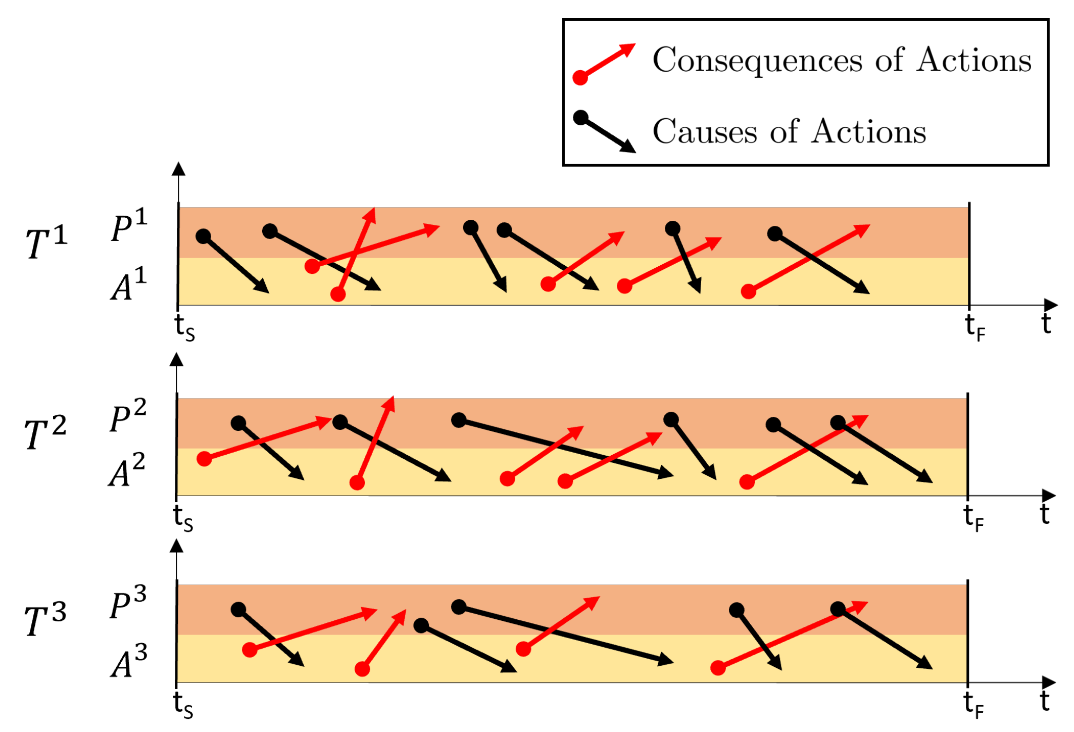
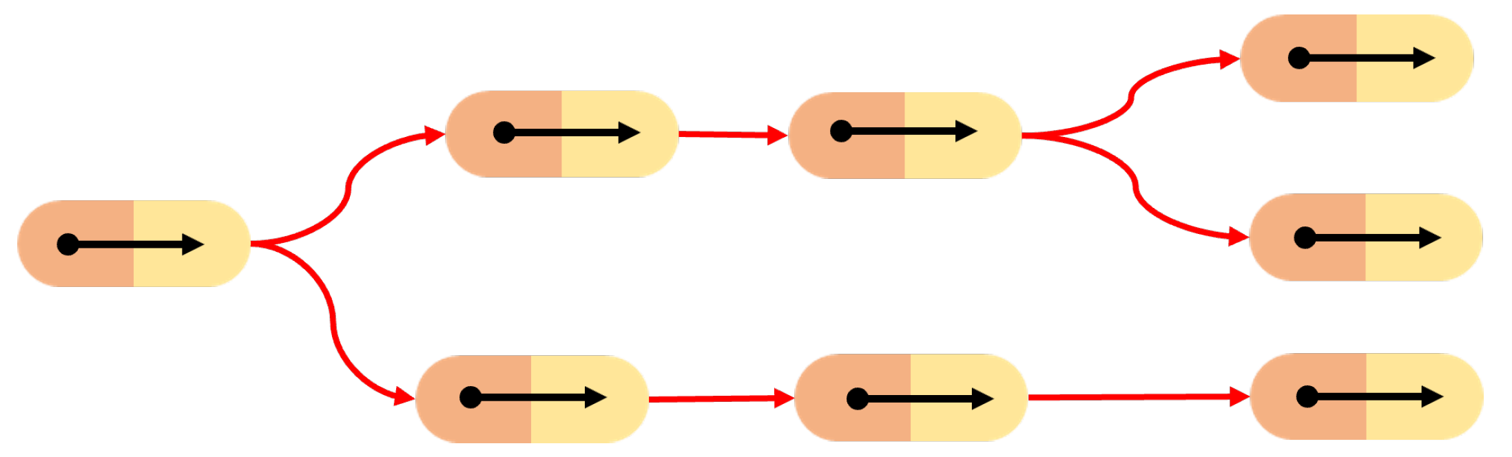
It is important to state that a core aspect of the problem is that of modeling and managing the temporal causality relations that regulate sensorimotor interactions (see Figure 1). However, based on our previous assumptions, we claim that the specifications of the m tasks are fully encoded in the n SMTs; therefore, our aim is to devise an algorithm to abstract the SMCs underlying the recorded SMTs, i.e., to devise a representation that models (i) which perceptions cause a given action (and its modality), and (ii) what are the consequences that can be expected when a given action is undertaken, i.e., that models the contingency relations between perceptions and actions. This SMC-based representation (see Figure 2) allows the robot to anticipate the future states based on current actions and perceptions in order to autonomously operate in novel, yet similar, contexts replicating the m tasks.

This problem is inherently complex for several reasons. Firstly, SMTs involve numerous continuous signals, necessitating the creation of a robust strategy to effectively handle the wealth of information associated with these signals while efficiently managing memory resources. Additionally, new contexts are unlikely to be exact duplicates of memorized SMTs. Consequently, the robot must possess the capability to assess the dissimilarities between different contexts and generalize the action component of the contingent sensorimotor trace to accommodate variations in the task arising from differences in the context itself. Merely reproducing memorized actions would be insufficient and impractical. Our objective requires that the robot (i) perceives the context in which it operates, (ii) identifies the matching SMC for that context, and (iii) acts accordingly within the current context based on the identified SMC.

3. Proposed Solution

When looking for SMCs, we aim to identify consistent causal relations between actions, perceptions, and given contexts. Therefore, to formulate a definition of SMC, it is necessary to formally define what is a context.

Building on Maye and Engel’s discrete history-based approach [5], we define the context of the robot–environment interaction at a given time $t^{\ast }$ as the historical record of all robot perceptions and actions starting from an initial time, $t_S$, expressed as:

$$c\left(t^{\ast }\right)\triangleq \left(P\left(t\right),A\left(t\right)\right):[t_S,t^{\ast }]\to \mathbb{U}\times \mathbb{P}.$$

(5)

It is important to note that while Equations (5) and (2) may seem similar, they differ significantly. Equation (2) represents a fixed set of actions and perceptions recorded within a specific past interval, while Equation (5) is dynamic, depending on the current time, $t^{\ast }$, and evolving over time.

Our method comprises several objectives, including (i) matching the present context with a memorized SMT, (ii) reproduce the behavior of the matched SMT, by (iii) adapting its actions to the current context, all based on (iv) a comparison between perceptions.

To accomplish this, our approach requires the introduction of the following components:

• A metric to measure the distance between perceptions $d_P(P_1\left(t\right),P_2\left(t\right))$ and actions $d_A(A_1\left(t\right),A_2\left(t\right))$;
• Contingency relations between SMTs, denoted as $C_T(T^1,T^2)$ and between a context and a SMT, denoted as $C_C(c,T)$;
• An operation to adapt an action to a different context.
  $A_{\ast }\left(t\right)=M(T_0,c_{\ast },t)=M((P_0\left(t\right),A_0\left(t\right)),c_{\ast },t)$.

It is important to note that defining and evaluating metrics such as $d_P$, $d_A$, $C_T$, $C_C$, and the operation M, can be a complex task, as they operate on functions of time defined over continuous intervals in multi-dimensional spaces. Our solution simplifies this challenge by identifying a discrete and finite set of instants, denoted as $t^{i,j}$ (for an i-th SMT and a j-th instant), within each interval in both the perception and action spaces. This mechanism, which we refer to as saliency, allows each SMT to be segmented into a sequence of $k^i$ SMT fragments, defined as:

$$T^{i,j}=\left(P^{i,j}\left(t\right),A^{i,j}\left(t\right)\right):[t^{j-1},t^j]\to \mathbb{U}\times \mathbb{P},$$

(6)

where most of the contingency relations between action and perception are concentrated, as illustrated in Figure 3.

Given a spatial distance in the task space $d_X(x^1,x^2)$, a distance between perceptions $D_P(P^1\left(t\right),P^2\left(t\right))$, and a distance between actions $D_A(A^1\left(t\right),A^2\left(t\right))$, the definition of a saliency let us introduce a contingency relation between SMTs $C_T(T^1,T^2)$, and a contingency relation between a context and an SMT $C_C(c,T)$. Moreover, leveraging the tools of Dynamic Movement Primitives (DMPs) [39], we defined a suitable contingency map $M(T_0,c_{\ast },t)$ such that $d_c(c_{\ast },(P_{\ast },M(T_0,c_{\ast },t)))=0$. With these distances and mapping operations established in an accessible form, the notion of saliency facilitates the creation of a discrete tree structure that models causal relations by using a discrete history-based approach, similar to that in [5]. In this tree, each directed edge corresponds to an SMC extracted from an SMT fragment, along with its saliency characterization, and nodes represent decision points. Given this SMC-tree, the system gains the ability to operate autonomously in new contexts by (i) comparing the current context with its memory using saliency, within the tree nodes to identify the best-matching SMC, and (ii) adapting the identified SMC to the present context. As we will see in the following sections, the introduction and definition of these metrics, essential for extracting salience and establishing contingency relationships, enable the system to handle various types of tasks effectively.

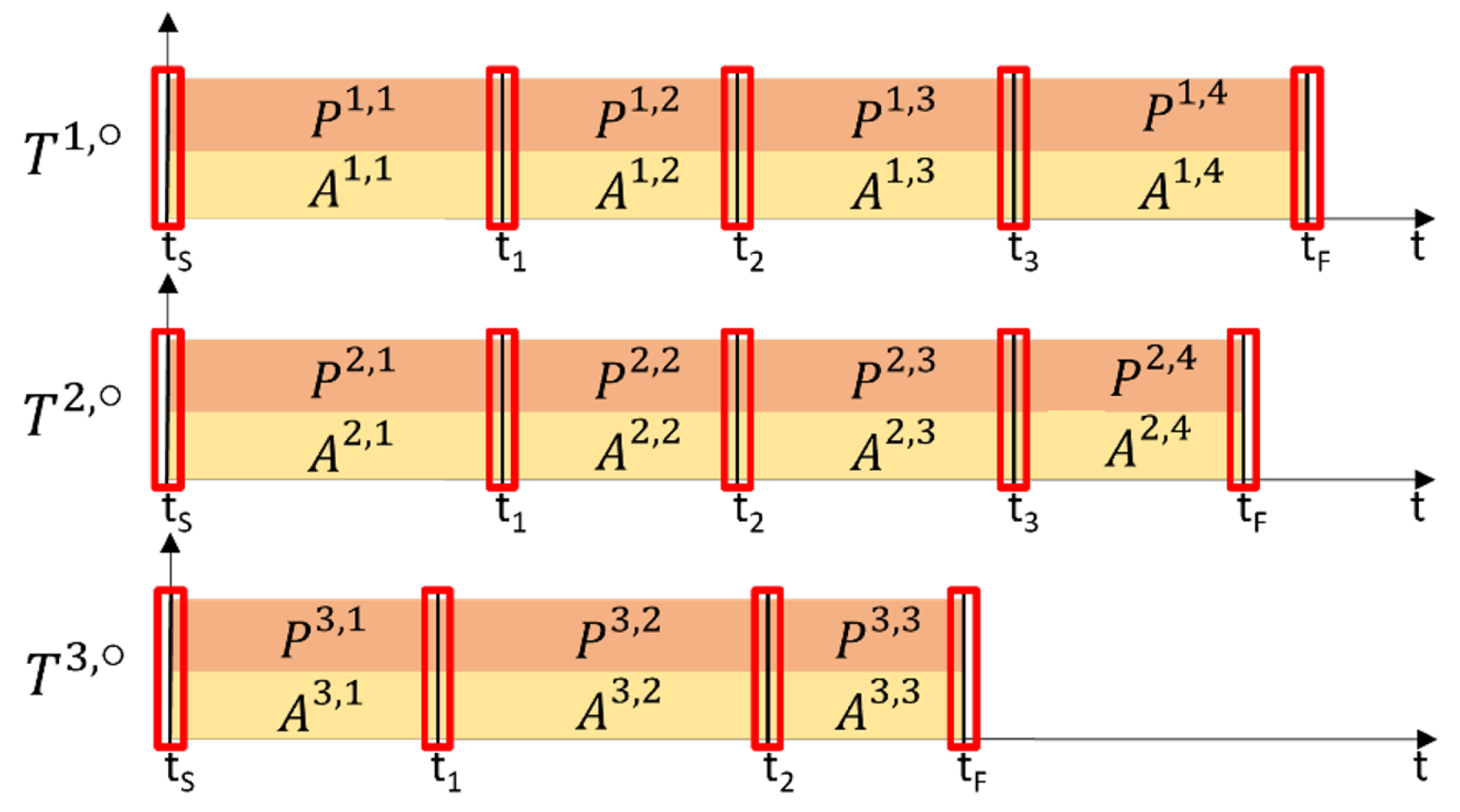
3.1. Temporal Saliency

In the work [23], the authors propose incorporating an attention mechanism to expand upon their previously introduced discrete approach for handling continuous signals. This attention mechanism is what we refer to as a form of temporal salience. It could be argued that temporal salience is inherent to SMTs themselves. The literature has offered various tools to enable artificial agents to extract temporal saliency from data. These techniques include Unsupervised Clustering [40], which groups similar actions into clusters based on features like joint angles, end effector positions, and tool usage; Hidden Markov Models [41], which identify distinct tasks in a sequence by modeling transitions between actions and estimating the probability of each task occurring; and Gaussian Mixture Models [42], which are probabilistic models that recognize different tasks by estimating Gaussian distribution parameters for each task.

Alternatively, temporal saliency can be explicitly communicated by the operator, either through verbal or visual cues or by manual activation of a trigger. In our experiments, as described in the following sections, we combine both automatic and explicit processes for extracting temporal salience.

This approach results in the division of each SMT $T^i$ into a collection of atomic SMT fragments, defined as:

$$T^i\triangleq \left(T^{i,1},...,T^{i,N}\right),$$

(7)

where each

$$T^{i,j}=T^{i,j}\left(t\right):\left[t_{j-1},t_j\right]\to \mathbb{U}\times \mathbb{P}=T^i{\left(t\right)|}_{\left[t_{j-1},t_j\right]}$$

(8)

is simply the restriction of the SMT to the interval $\left[t_{j-1},t_j\right]$.

By analogy, we refer to the perception and action components of each sub-task as $P^{i,j}$ and $A^{i,j}$, respectively.

3.2. Spatial Saliency

To extract salient information for both perceptions and actions, we must identify the robot’s state during the recording of a SMT. This is achieved by considering a $x_{POI}$, which represents a point of interest for the robot. For instance, in the case of a robot’s end-effector, $x^{EE}\in {\mathbb{X}}_1$ is a typical choice. For a mobile robot, its state is represented as $\mathbf{x}=(x,y,\theta )\in {\mathbb{X}}_2$.

The temporal evolution of $x_{POI}$ is an integral part of the action stream recorded in the SMT.

As we will see in the following sections, particularly in the context of perceptions, $x_{POI}$ plays a pivotal role in narrowing the focus to perceptions in close proximity to the robot, as detailed in Section 3.3.

On the other hand, when it comes to actions, this variable serves a dual purpose. Not only does it assist in extracting the saliency of actions, but it also facilitates their adaptation to new contexts, as explained in Section 3.4.

3.3. Perception Saliency and Inter-Perception Distance

To provide a comprehensive introduction to the concept of perception saliency, it is essential to begin by categorizing perceptions. In the field of robotics, many types of sensors find common uses, including optical sensors like cameras, LiDAR, and depth sensors, as well as force sensors such as load cells, torque sensors, and tactile sensors. Additionally, distance sensors like ultrasonic, infrared, and LIDAR, as well as temperature and proximity sensors, play vital roles. Each of these sensors generates distinct types of raw data, ranging from images to scalar values and point clouds, and each offers a unique perspective on either the environment or the robot itself. This diversity necessitates a structured approach to organize and enhance the saliency process.

Within the realm of sensory perception, two fundamental categories emerge: intrinsic and extrinsic perceptions. Intrinsic perception entails using a sensor to gain insights into the properties of the sensor itself, while extrinsic perception involves employing the sensor to understand the properties of the surrounding environment.

A simple intrinsic (SI) perceptual signal ${}_b\tilde{p}\in {}_b\mathbb{P}$ is a perceptual signal that admit a (sensorial perception) distance function

$${}_{b}d_P({}_b\tilde{p}^1,{}_b\tilde{p}^2):{}_b\mathbb{P}\times {}_b\mathbb{P}\to {\mathbb{R}}_{0+}.$$

(9)

Note that here and in the following, the right superscript does not indicate a power, it is an index. Examples of simple intrinsic perceptual signal are, e.g., an environmental temperature sensor that measures the temperature in Kelvin degrees, for which ${}_b\tilde{p}=T\in R_{0+}$ and ${}_{b}d_P({}_b\tilde{p}^1,{}_b\tilde{p}^2)=|{}_b\tilde{p}^2-{}_b\tilde{p}^1|$ or the joint torques vector of a robot ${}_b\tilde{p}=q\in R^n$, which can use the distance defined, e.g., by the $L_2$-norm:

$${}_{b}d_P({}_b\tilde{p}^1,{}_b\tilde{p}^2)=\sqrt{{({}_b\tilde{p}^2-{}_b\tilde{p}^1)}^T({}_b\tilde{p}^2-{}_b\tilde{p}^2)}.$$

(10)

A simple extrinsic or localized (SL) perceptual signal ${}_b\overline{p}\in {}_b\overline{\mathbb{P}}$, instead, is defined as a pair of an intrinsic perception and a location ${}_{b}x\in \mathbb{X}$

$${}_b\overline{p}=\left({}_b\tilde{p},{}_{b}x\right)\in {}_b\mathbb{P}\times \mathbb{X}.$$

(11)

Since simple localized perceptions contain intrinsic perception, they must admit a sensorial perception distance function too

$${}_{b}d_P({}_b\overline{p}^1,{}_b\overline{p}^2)\triangleq {}_{b}d_P({}_b\tilde{p}^1,{}_b\tilde{p}^2):{}_b\mathbb{P}\times {}_b\mathbb{P}\to {\mathbb{R}}_{0+},$$

(12)

and, due to the location, a spatial distance function

$${}_{b}d_X({}_b\overline{p}^1,{}_b\overline{p}^2)\triangleq {}_{b}d_X({}_{b}x^1,{}_{b}x^2):\mathbb{X}\times \mathbb{X}\to {\mathbb{R}}_{0+}.$$

(13)

Examples of localized signals are the triangulated echo of an object sensed through a sonar sensor, or a segmented point-cloud extracted from the image of a depth camera. This type of perception (SL) can also be multiple, ML, when it does not assume a unique value but a set of values simultaneously. We define a multiple localized perceptual signal as a finite set of variable size of localized perceptual signal, that is

$${}_b\overline{p}_{\circ }=\left\{{}_b\overline{p}_1,{}_b\overline{p}_2,\dots ,{}_b\overline{p}_{n_m}\right\}\mathrm{where}{}_b\overline{p}_j\in {}_b\overline{\mathbb{P}}$$

(14)

which admit a sensorial perception distance

$${}_{b}d_P({}_b\overline{p}_{\circ }^1,{}_b\overline{p}_{\circ }^2)\triangleq {}_{b}d_P({}_b\tilde{p}_{\circ }^1,{}_b\tilde{p}_{\circ }^2):{}_b\mathbb{P}_{\circ }\times {}_b\mathbb{P}_{\circ }\to {\mathbb{R}}_{0+}.$$

(15)

where ${}_b\tilde{p}_{\circ }^k$ in Equation (15) represents the intrinsic perceptions part of ${}_b\overline{p}_{\circ }^k$.

After outlining the various types of perceptions, we employ this classification to define a distinct salient sub-set for each sub-task

$${}^{S}P^{i,j}\subseteq P^{i,j}.$$

(16)

This is achieved by applying the following rules for extracting perception saliency:

(a)

Given a simple intrinsic perception $P^{i,j}={}_b\tilde{p}^{i,j}$ or a set of intrinsic perceptions $P^{i,j}=\left({}_b\tilde{p}^{i,j}\right)$, all the intrinsic perceptions are considered candidate

$${}_b\tilde{p}^{i,j}\in {}^{S}P^{i,j}$$

(17)

(b)

Given a simple localized perception $P^{i,j}=\left({}_1\overline{p}^{i,j}\right)$

$${}_1\overline{p}^{i,j}\in {}^{S}P^{i,j}\iff {}_{1}d_X({}_{1}x^{i,j},x_{POI})<{}_1ϵ$$

(18)

where ${}_1ϵ\in {\mathbb{R}}_{+}$ is an appropriate threshold value for a specific sensor.

(c)

Given a set of simple localized perceptions $P^{i,j}=({}_1\overline{p}^{i,j},\dots ,{}_n\overline{p}^{i,j})$

$${}_k\overline{p}^{i,j}\in {}^{S}P^{i,j}\iff {}_{k}d_X({}_{k}x^{i,j},x_{POI})<{}_kϵ$$

(19)

where

$$k=arg\underset{k=1,\dots ,n}{min}\left({}_{k}d_X({}_{k}x^{i,j},x_{POI})\right)$$

(20)

(d)

Given a multiple localized perception $P^{i,j}=\left({}_1\overline{p}_{\circ }^{i,j}\right)=\left(\{{}_1\overline{p}_1^{i,j},\dots ,{}_1\overline{p}_m^{i,j}\}\right)$

$${}_1\overline{p}_l^{i,j}\in {}^{S}P^{i,j}\iff {}_{1}d_X({}_{1}x_l^{i,j},x_{POI})<{}_1ϵ$$

(21)

where

$$l=arg\underset{l=1,\dots ,m}{min}\left({}_{l}d_X({}_{1}x_l^{i,j},x_{POI})\right)$$

(22)

(e)

Given a set of multiple localized perception $P^{i,j}=({}_1\overline{p}_{\circ }^{i,j},\dots ,{}_h\overline{p}_{\circ }^{i,j})$

$${}_k\overline{p}_l^{i,j}\in {}^{S}P^{i,j}\iff {}_{k}d_x({}_{\mathrm{k}}x_l^{i,j},x_{POI})<{}_1ϵ$$

(23)

where

$$l=arg\underset{l=1,\dots ,r}{min}\left({}_{l}d_X({}_{\mathrm{k}}x_l^{i,j},x_{POI})\right),k=1,\dots ,h$$

(24)

$$k=arg\underset{k=1,\dots ,h}{min}\left({}_{l}d_X({}_{\mathrm{k}}x_l^{i,j},x_{POI})\right)$$

(25)

r denotes the elements number of ${}_k\overline{p}_{\circ }^{i,j}$, that could be different for each multiple perception.

In general, the perceptions within each SMT fragment, denoted as $P^{i,j}=p^{i,j}$, encompass a mix of different perceptions falling into three distinct categories (SI, SL, and ML). Consequently, the previously mentioned rules are applied to the relevant type of perception under consideration.

The outcome of the perception saliency process is the generation of a sequential set of salient perceptions ${}^{S}P^{i,j}$, for each SMT fragment $T^{i,j}=(P^{i,j},A^{i,j})$.

Lastly, the computation of the inter-perception distance $D_P$, between two sets of sub-task perceptions, $P^{1,j}$ and $P^{2,j}$, which must contain the same number and types of perceptions, is facilitated through their salient perceptions. This is expressed as:

$$D_P(P^{1,j},P^{2,j})=D_P({}^{S}P^{1,j},{}^{S}P^{2,j})=\underset{b}{\oplus }{}_{b}d_P({}_b{}^{S}p^{1,j},{}_b{}^{S}p^{2,j})$$

(26)

where the symbol ⊕ represents the summation of various distances, taking into account the different categories (e.g., between intrinsic and localized perceptions) and includes appropriate normalization. It is important to note, in conclusion, that the saliency of localized perceptions is also influenced by the variable $x_{POI}$, as discussed in Section 3.2.

3.4. Action Saliency and Inter-Action Distance

The action associated with the j-th fragment of the i-th SMT is encoded using a parametric function that represents its salient features:

$${}^{S}A^{i,j}({\omega }^{i,j},x_s,x_f,\tau ):\mathbb{W}\times \mathbb{X}\times \mathbb{X}\times \mathbb{T}.\to \mathbb{U}$$

(27)

This encoding is employed for adapting the action to a different context during autonomous execution. Here are the key components of the action encoding:

• ${\omega }^{i,j}$ is a parameterization of the salient action.

  $${\omega }^{i,j}=f_{\omega }\left(A^{i,j}\left(t\right)\right):[t_{j-1},t_j]\to \mathbb{W}$$

  (28)

  where $f_{\omega }\left(\right)$ is a function that encodes the action $A^{i,j}\left(t\right)$ in the time interval $[t_{j-1},t_j]$. In this work, we use the DMP method to encode the robot’s movement.
• $x_s$ is an empty variable which will be replaced by $x_{POI}$ in the starting configuration during the autonomous execution, e.g., the end-effector pose $x_{EE}$ or the state x, before executing the learned action.
• $x_f$ stands for the final value that $x_{POI}$ will assume at the end of sub-task. This value depends on the type of perceptions involved. If only salient intrinsic perceptions are at play, then $x_f=x_{POI}\left(t_j\right)$, with $x_{POI}\left(t_j\right)$ denoting the final value assumed by $x_{POI}$ at the end of the j-th subtask during the SMT registration. Conversely, if at least one localized perception is involved, $x_f$ becomes parameterized with the perception’s location, as explained in the Contingent Action Mapping section (Section 3.6).

Similar to the inter-perception distance, we define the inter-action distance $D_A$ between two distinct sub-task actions $A^{1,j}$, $A^{2,j}$ based on their saliency actions ${}^{S}A^{1,j},{}^{S}A^{2,j}$:

$$D_A({}^{S}A^{1,j},{}^{S}A^{2,j})=d_a({\omega }^{1,j},{\omega }^{2,j})$$

(29)

where $d_a$ is the euclidian distance function applied to the action parametrization, drawing inspiration from [43]. In particular, regarding Equation (29), when given two parameterizations ${\omega }^{1,j}$ and ${\omega }^{2,j}$ of two actions, their inter-action distance is equal to zero if and only if the two parametrizations are the same:

$$d_a({\omega }^{1,j},{\omega }^{2,j})=0\iff {\omega }^{1,j}={\omega }^{2,j}.$$

(30)

3.5. Contingency Relation

Now that we have established the categories of perceptions and the essential attributes needed to characterize a Sensory-Motor Trace (SMT), we can delve into defining two types of contingency relations: $C_T$ between two SMTs and $C_C$ between a context and an SMT.

Starting with two distinct SMTs, denoted as $(T^1,T^2)$, each characterized by temporal saliency $(T^{1,j},T^{2,j})$, perception saliency $({}^{S}P^{1,j},{}^{S}P^{2,j})$, and action saliency $({}^{S}A^{1,j},{}^{S}A^{2,j})$, we establish their contingency based on the contingency relation between their constituent fragments. Therefore, two fragments, $(T^{1,j},T^{2,j})$, are considered contingent if the following contingency fragment relation $C_F(T^{1,j},T^{2,j})$ holds true:

$$C_F(T^{1,j},T^{2,j})=D_A({}^{S}A^{1,j},{}^{S}A^{2,j})<T_{h_A}\wedge D_P({}^{S}P^{1,j},{}^{S}P^{2,j})<T_{h_P}$$

(31)

where $T_{h_A}$,$T_{h_P}$ are the thresholds, respectively, for the distance between actions and perceptions.

To determine the contingency between two SMTs, $T^1$ and $T^2$, we declare $C_T(T^1,T^2)$ as True if and only if all pairs of fragments $(T^{1,j},T^{2,j})$ satisfy the contingency condition:

$$C_T(T^1,T^2)=True\iff C_F(T^{1,j},T^{2,j}):\forall j$$

(32)

Now, to establish contingency between an SMT and a context, we must first extract saliency from the context. Given a context $c\left(t^{\ast }\right)$, the process of temporal saliency extraction results in a collection of context fragments denoted as:

$$c\left(t^{\ast }\right)\triangleq \left({c_{\ast }}^1,\dots ,{c_{\ast }}^{N_c-1},{c_{\ast }}^{N_c}\right),$$

(33)

where each ${c_{\ast }}^j$ represents a fragment:

$${c_{\ast }}^j={c_{\ast }}^j\left(t\right):\left[t_{j-1},t_j\right]\to \mathbb{U}\times \mathbb{P}=c_{\ast }{\left(t\right)|}_{\left[t_{j-1},t_j\right]}$$

(34)

This process is analogous to the task segmentation described earlier, with the notable distinction that the number of context fragments increases over time, and the most recent fragment ${c_{\ast }}^{N_c}$ is always associated with the current time $t^{\ast }$. Each sub-context’s perception and action components are identified as ${P_{\ast }}^j$ and ${A_{\ast }}^j$, respectively. Saliency is then extracted from these components as ${}^S{P}_{\ast }^j$ for perceptions and ${}^S{A}_{\ast }^j$ for actions, following the methodology previously outlined.

To evaluate the contingency between a context $c\left(t^{\ast }\right)$ and an SMT $T^i$, we consider that through the extraction of temporal saliency, the context aligns with an SMT for all instances prior to the current one (i.e., $j<N_c$). The key difference lies in evaluating the present instance, ${c_{\ast }}^{N_c}$. Therefore, for a context to exhibit contingency with an SMT, the contingency relationship between SMT fragments should hold for the past history, as follows:

$$C_{Past}({c_{\ast }}^j,T^{i,j})=True\iff C_F({c_{\ast }}^j,T^{i,j}):\forall j<N_c$$

(35)

Moreover, the contingency condition in the current instance, denoted as $C_{Now}$, must be met, taking into account the saliency of perceptions only:

$$C_{Now}({c_{\ast }}^{N_c},T^{i,N_c})=D_P({}^S{P_{\ast }}^{N_c},{}^{S}P^{i,N_c})<T_{h_P}.$$

(36)

Thus, for a new context and an SMT to be considered contingent, $C_C({c_{\ast }}^j,T^{i,j})=True$, they must exhibit contingency both in the past and in the current instance:

$$C_C({c_{\ast }}^j,T^{i,j})=True\iff C_{Past}({c_{\ast }}^j,T^{i,j})\wedge C_{Now}({c_{\ast }}^{N_c},T^{i,N_c})$$

(37)

It is important to note that when the current instance aligns with the initial starting time $t^{\ast }=t_S$ (in discrete time, $j=N_c$), the contingency relation between a context and an SMT simplifies to solely the present contingency condition $C_C({c_{\ast }}^j,T^{i,j})=True\iff C_{Now}({c_{\ast }}^{N_c},T^{i,N_c})$.

In conclusion, it is worth emphasizing that we exclusively take into account the salient perceptions to assess contingency at the current instant. This choice aligns with our goal of identifying and retrieving the action component from the stored SMTs, which, in turn, enables us to adapt the action to the current context, as explained in the following section.

3.6. Contingent Action Mapping

Given a context denoted as $c\left(t^{\ast }\right)$ and a contingent SMT fragment represented by $T^{i,j}=(P^{i,j},A^{i,j})$, we introduce a contingent mapping function $M(T^{i,j},c_{\ast },t)$ to determine a new action $A_{\ast }\left(t\right)$ to be executed at the current time $t^{\ast }$. This new action is derived from the adaptation of the salient action ${}^{S}A^{i,j}$ to the context $c\left(t^{\ast }\right)$, with the aim of minimizing the distance $D_A(A_{\ast }\left(t\right),{}^{S}A^{i,j})$, provided that (37) is satisfied.

Moreover, the design of this new action $A_{\ast }\left(t\right)$ is such that, when applied, it ensures that the resulting updated context $c(t^{\ast }+1)$ continues to be contingent in the past to the corresponding SMT, as described in Equation (35). This definition allows us to state that upon the successful autonomous execution and adaptation within the current context of an SMT $T^i$ stored in the tree, the resultant SMT $\widehat{T^i}$ is contingent upon $T^i$, meaning that $C_T(T^i,\widehat{T^i})$ evaluates to True.

Mathematically, this new action $A_{\ast }\left(t\right)$ can be expressed as:

$$\begin{array}{c}\hfill A_{\ast }\left(t\right)=M(T^{i,j},c_{\ast },t)=M((P^{i,j},A^{i,j}),({P_{\ast }}^{N_c},{A_{\ast }}^{N_c}),t)=\\ \hfill M(({}^{S}P^{i,j},{}^{S}A^{i,j}),({}^S{P_{\ast }}^{N_c},{}^S{A_{\ast }}^{N_c}),t)={}^{S}A^{i,j}({\omega }^{i,j},x_{POI}\left(t^{\ast }\right),x_f^{\ast },\tau )\end{array}$$

(38)

where the value of $x_f^{\ast }$ depends on the type of perceptions involved in ${}^S{P_{\ast }}^{N_c}$ and ${}^{S}P^{i,j}$. It is important to note that these perceptions must be of the same type and number to be compared. If they only contain intrinsic perceptions, then $x_f^{\ast }$ is equal to the final value assumed by $x_{POI}$ at the end of $T^{i,j}$, $x_{POI}\left(t_j\right)$. However, if they involve a localized perception, $x_f^{\ast }$ assumes the value ${}_b{x}^{N_c}$ associated with the location of the localized perception pair (${}_l{}^S{p}^{N_c},l{x}^{N_c}$) in ${}^S{P}^{N_c}$, having the minimum distance from the salient localized perception ${}^S{\overline{p}}^{i,j}\in {}^S{P}^{i,j}$:

$$arg\underset{l=1,..,s}{min}{}_{b}d_P({}_l{}^S{p}^{N_c},{}^S{\overline{p}}^{i,j})$$

(39)

where s represent the localised perception cardinality.

3.7. Sensory-Motor Contingency

As previously discussed, after formally defining the contingency relationships between two SMTs and an SMT with the context through the extraction of perceptual and action salience, we can now introduce the concept of an SMC (Sensory-Motor Contingency). An SMC is defined as the pair of salient perceptions and actions for an SMT fragment obtained through temporal saliency extraction.

For a given sensory-motor trace $T^i$ and its corresponding fragments $T^{i,j}$, we define a sensorimotor contingency SMC as:

$$S^{i,j}=({}^S{P}^{i,j},{}^S{A}^{i,j})$$

(40)

and

$$S^i\triangleq \left(S^{i,1},\dots ,S^{i,N}\right)$$

(41)

is the set of SMCs associated with $T^i$.

It is important to note that since all the metrics and relationships introduced earlier rely on the salience of SMT, they naturally pertain to the SMC. This definition enables us to represent the connections between actions and changes in perceptions as a discrete tree structure, where each edge represents an SMC, and each node represents a decision point. These decision points, denoted as $\Pi$, are intances where temporal salience was extracted. During autonomous execution, an assessment of the tree is required to evaluate the execution of future actions by identifying the most context-contingent SMC among all the SMCs in the tree.

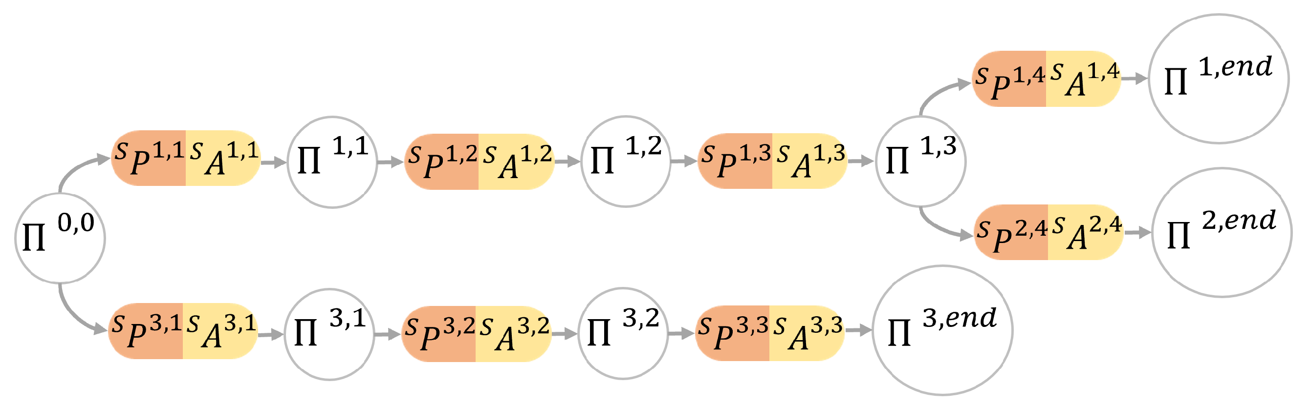
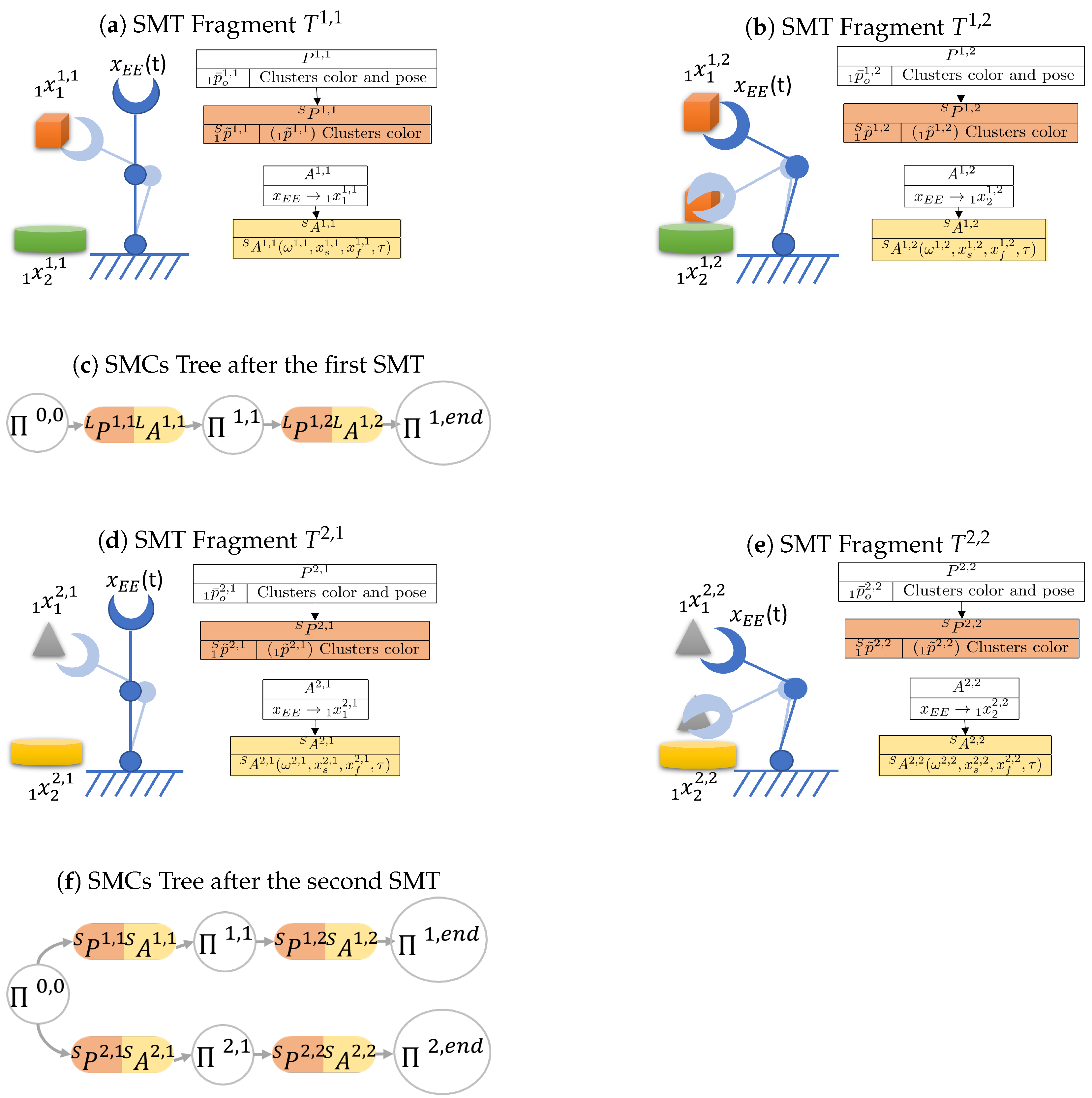
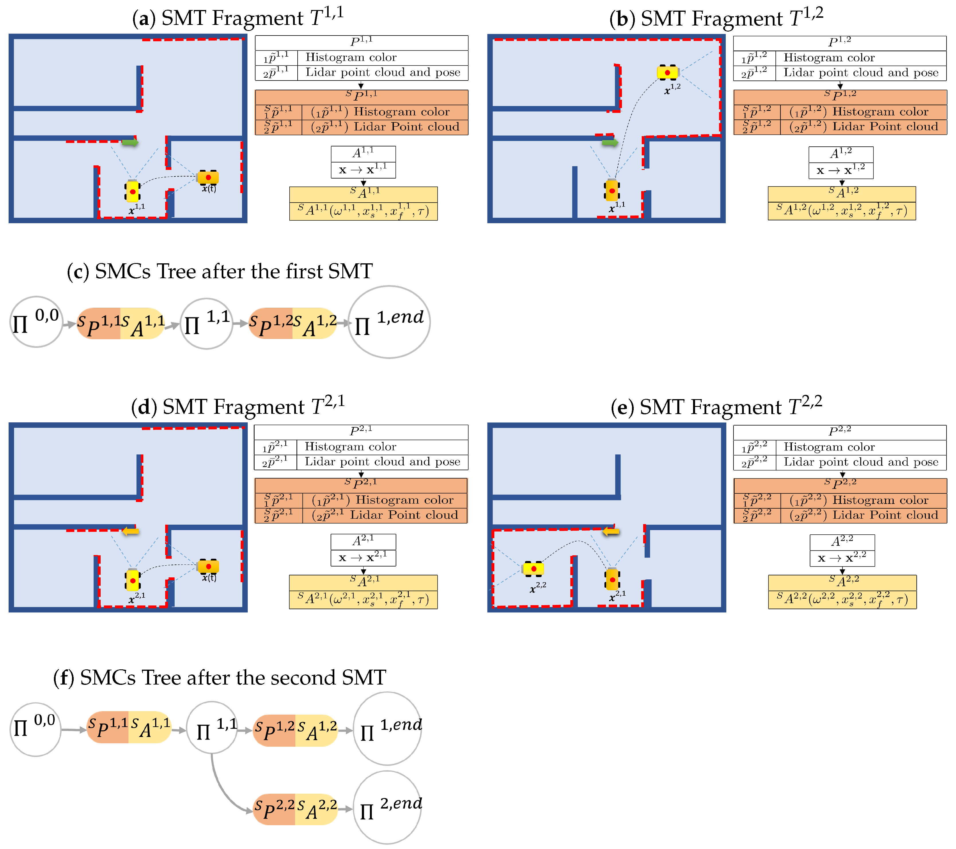
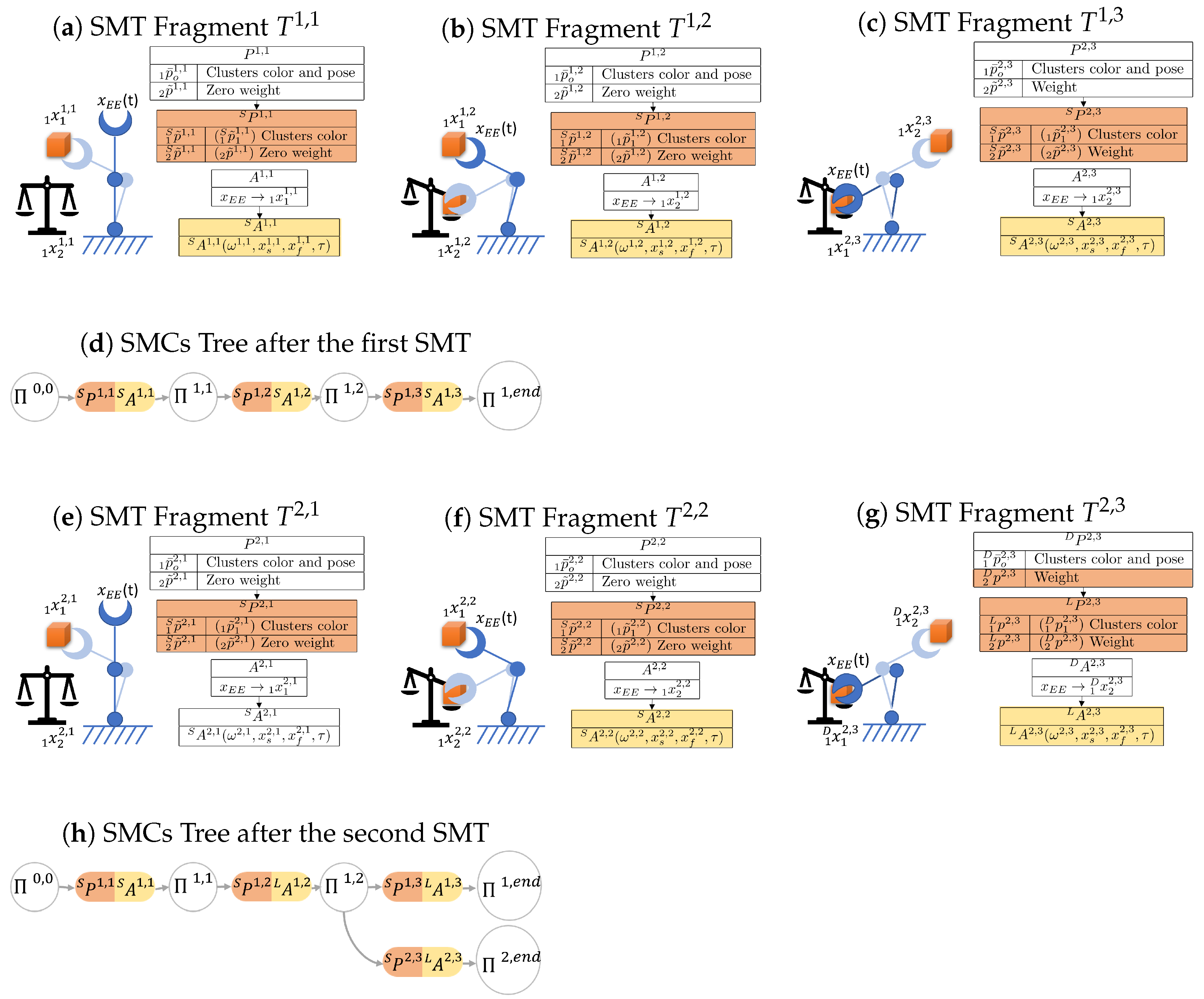
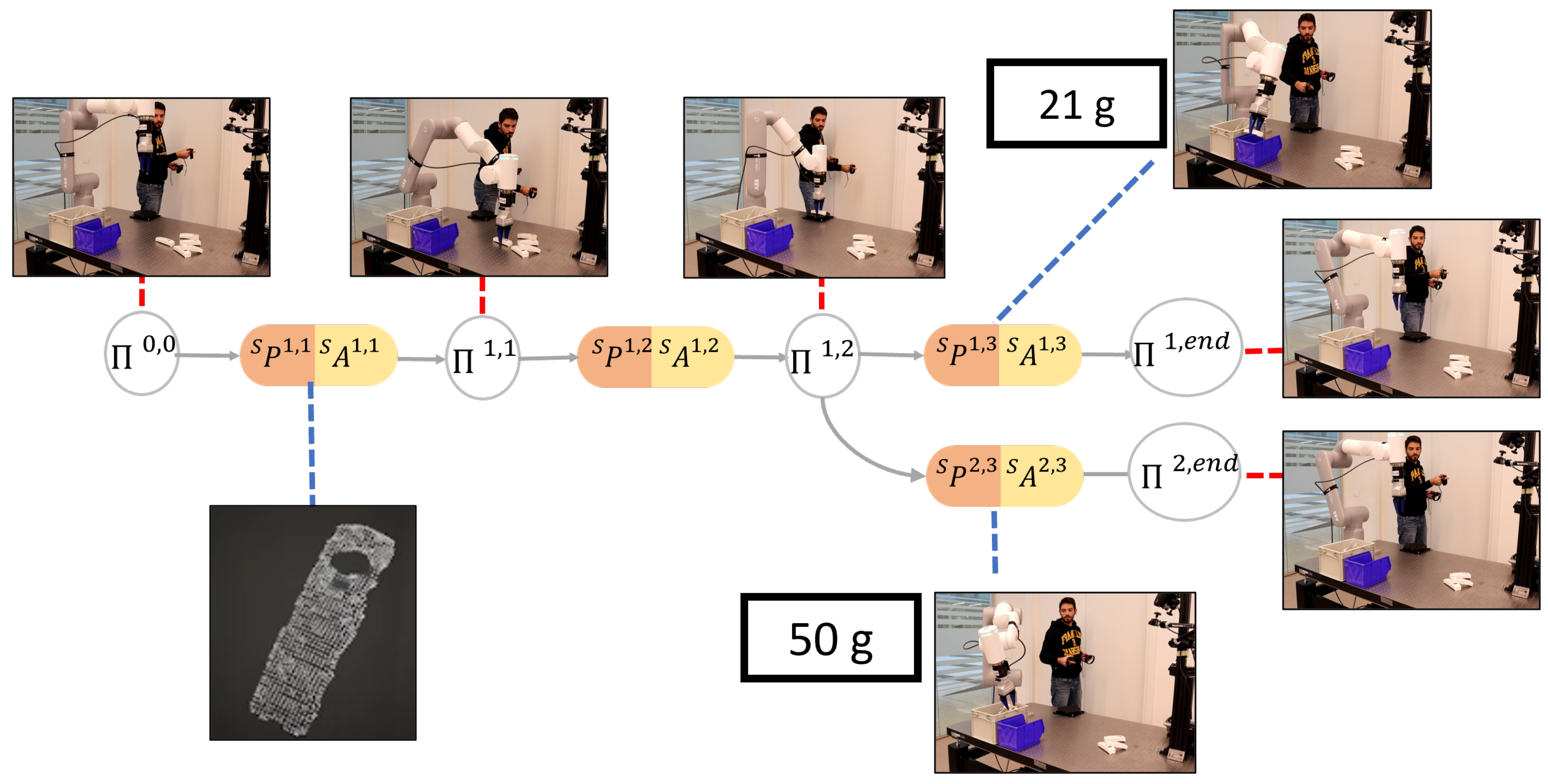
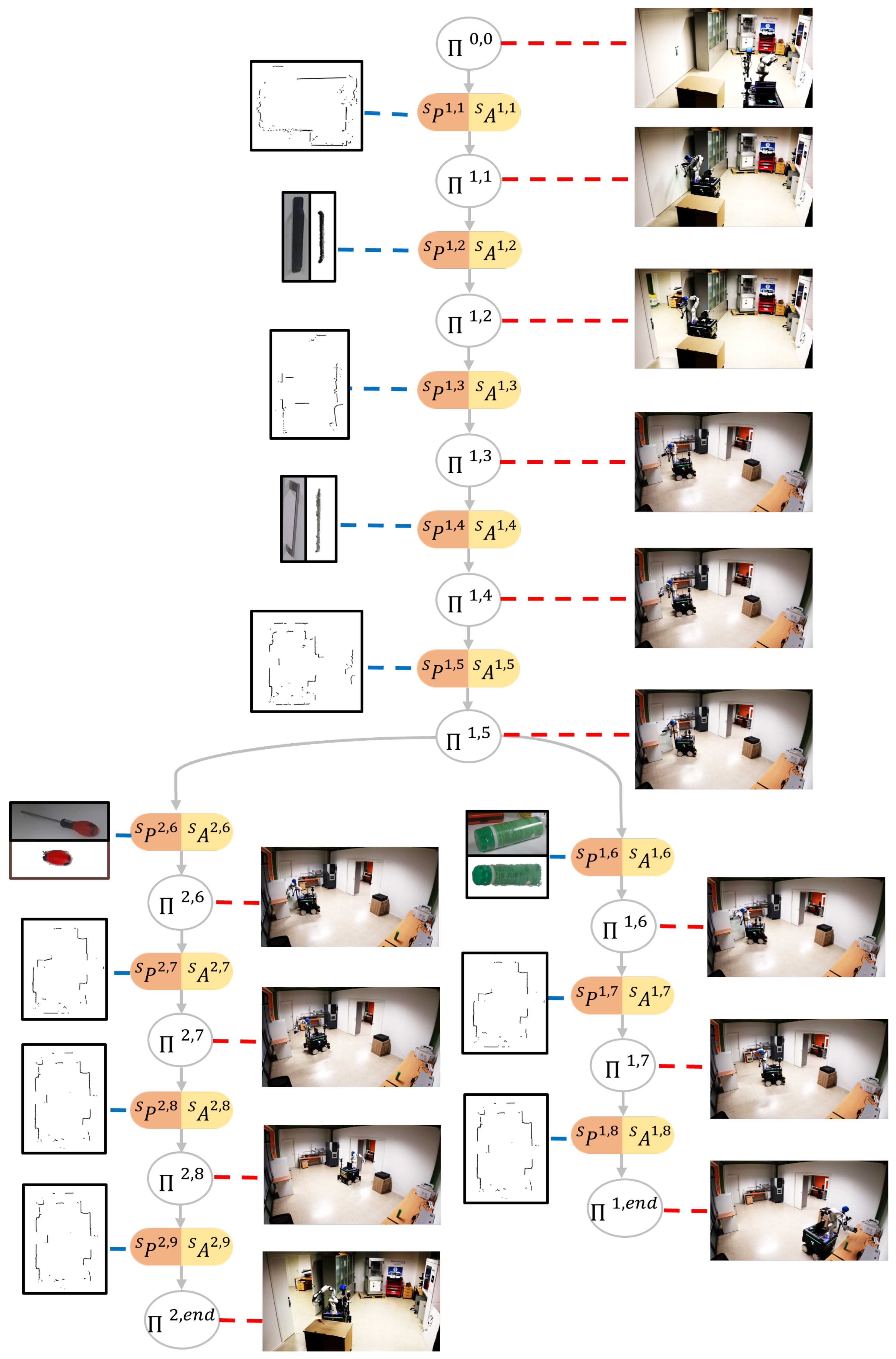
3.8. Sensory-Motor Contingencies Tree

The method for constructing the SMCs tree follows the algorithm presented in Algorithm 1. To build this tree, each SMT is processed by extracting its saliency following the procedure in Section 3.3 and Section 3.4. If the tree is initially empty, the first SMT is automatically stored, and the first branch is added to the tree. Otherwise, a process is executed to efficiently incorporate a new SMT into the existing tree. This procedure enables the integration of initial SMC candidates from a novel SMT with specific branches of previously stored SMTs. In essence, when elements of a new task exhibit similarities to those already stored, the system selectively archives only the distinct portions of the task. These distinct portions are then inserted into decision points associated with pre-existing SMTs.

Suppose the tree is composed of m branches, with each branch originating from the root node (as depicted in Figure 4). After extracting the SMC candidates for a new SMT denoted as $T^{\ast }$, a new branch is created, consisting of N SMCs to be included in the existing SMC tree:

$$\{S^{\ast ,1},\dots ,S^{\ast ,N}\}=\{({}^S{P}^{\ast ,1},{}^S{A}^{\ast ,1}),\dots ,({}^S{P}^{\ast ,N},{}^S{P}^{\ast ,N})\}$$

(42)

where ∗ denotes the new branch.

At each step, the process evaluates the contingency SMT fragment relationship between $S^{\ast ,j}$ and the SMCs $S^{i,j}$ present in the tree, which are admitted by the node ${\Pi }^{h,j-1}$. This process begins with the initial step where $h=0$ and $j=1$. The equation for this contingency check is as follows:

$$C_F(S^{\ast ,j},S^{i,j}):\forall i\in {\mathbb{I}}_j$$

(43)

Here, ${\mathbb{I}}_j$ represents a set of all the SMCs indexes i admitted by the node ${\Pi }^{h,j-1}$.

If $S^{\ast ,j}$ is found to be contingent with $S^{i,j}$, then $S^{i,j}$ is added to the set $S_{con}$, which contains all $S^{i,j}$-contingent SMCs. Otherwise, the contingency check continues with the next SMC connected to ${\Pi }^{h,j-1}$.

After all SMCs to be compared have been examined, if $S_{con}$ remains empty, the new SMCs $S^{\ast ,k}:k=j,\dots ,N$ are connected to the node ${\Pi }^{h,j-1}$, and the check concludes. Otherwise, if $S_{con}$ is not empty, the process proceeds to assess the salient perceptions in $S_{con}$ to identify the most contingent SMC: the one with the least inter-perception distance. To identify it, the process computes the index that minimizes this distance:

$$i_{min}=arg\underset{i\in {\mathbb{I}}_j}{min}\left(D_P({}^S{P}^{\ast ,j},{}^S{P}^{i,j})\right)$$

(44)

After this, the process merges the SMCs $S^{\ast ,j}$ and $S^{i_{min},j}$, and the check continues on the branch identified by the index $i_{min}$. The process concludes once all the SMCs of the new branch have been processed. The merging between two SMCs can be performed in several ways, such as choosing one of them or applying other sensor fusion and trajectory optimization methods. The merging process can also be viewed as an opportunity for the robot to enhance its understanding of the same SMC. In cases where a particular task is repeated multiple times, during the merging process, the system can systematically merge all the Sensory-Motor Contingencies by consistently integrating the parameters of the older SMCs with the new ones. This iterative refinement allows the system to progressively improve its comprehension of the task, leveraging past experiences to enhance its performance.

Algorithm 1 SMCs Tree

1: function $[\Pi ]$ = $Build\_SMCs\_Tree$($T^{\ast },\Pi$) 2:     $[T^{\ast ,1},\dots ,T^{\ast ,N}]$ = $Extract\_temporal\_saliency\left(T^{\ast }\right)$ 3:     $[S^{\ast ,1},\dots ,S^{\ast ,N}]$ = $Extract\_SMCs\left([T^{\ast ,1},\dots ,T^{\ast ,N}]\right)$ 4:     if $\Pi$ is empty then ${\Pi }^{0,0}.append\left([S^{\ast ,1},\dots ,S^{\ast ,N}]\right)$ 5:     else 6:         $int$$h=0$ 7:         $int$$j=1$ 8:         $S_{con}=\left[\right]$ 9:         for all $S^{\ast ,j}$ in $[S^{\ast ,1},\dots ,S^{\ast ,N}]$ do 10:            for all $S^{i,j}$ admitted by ${\Pi }^{h,j-1}$ do 11:                if $C_F(S^{\ast ,j},S^{i,j})$then                                        ▹(43) 12:                    $S_{con}.append\left(S^{i,j}\right)$ 13:                end if 14:            end for 15:            if $S_{con}$ is not empty then 16:                Find $i_{min}\left(\right)$                                                       ▹(44) 17:                $Merge\_SMCs$($S^{\ast ,j},S^{i_{min},j}$) 18:            else 19:                ${\Pi }^{h,j-1}.append\left([S^{\ast ,j},\dots ,S^{\ast ,N}]\right)$ 20:                Return $\Pi$ 21:            end if 22:            $h=i_{min}$ 23:            $j++$ 24:         end for 25:     end if 26: end function

3.9. SMCs-Aware Control

During autonomous execution, the robot can operate in new contexts that are akin to those stored in the SMCs tree, and this is facilitated by Algorithm 2. The process begins at the initial decision point and proceeds along the identified branch of the tree, given that compatible perceptions are encountered along the way.

At each step within each decision point, the SMC control takes a new context denoted as $c\left(t^{\ast }\right)$, extracts the context’s saliency (as detailed in (33)), and seeks the most contingent SMC fragment within the SMC tree. The objective of this control is to generate a new action that ensures the past contingency of the subsequent context $c(t^{\ast }+1)$ with the identified branch of SMCs from the tree. Thus, during each step, the system evaluates only the current contingency between the context and the SMCs, $C_{Now}$, to determine the most contingent SMC. This assessment entails identifying the index $i_{min}$ as follows:

$$i_{min}=arg\underset{i\in {\mathbb{I}}_j}{min}\left(C_{Now}({c_{\ast }}^{N_c},S^{i,N_c})\right)$$

(45)

whereas, ${\mathbb{I}}_j$ represents a set of all the SMCs indexes i admitted by the node ${\Pi }^{h,j-1}$.

Once, the most contingent SMC is found, the index $i_{min}$ is employed in the contingent action mapping to compute $A_{\ast }\left(t\right)$:

$$\begin{array}{c}\hfill A_{\ast }\left(t\right)=M(T^{i_{min},N_c},c_{\ast },t)=\\ \hfill {}^S{A}^{i_{min},N_c+1}({\omega }^{i_{min},N_c},x_{POI}\left(N_c\right),x_f^{\ast },\tau ).\end{array}$$

(46)

Finally, if, during the execution, the system fails to establish any correspondence with the SMC-tree ($C_C({c_{\ast }}^j,T^{i,j})=False$), it has the option to resume the recording process and initiate the recording of a new SMT, starting from the ongoing execution.

Algorithm 2 Autonomous Execution

1: $j=1$ 2: $h=0$ 3: $Retrieve\_SMCs\_Tree\_\Pi \left(\right)$ 4: for all  ${\Pi }^{h,j-1}$  do 5:       $Perceive\_New\_Context\_c\left(t^{\ast }\right)$ 6:       $[{c_{\ast }}^1,\dots ,{c_{\ast }}^{N_c}]$ = $Extract\_temporal\_saliency\left(c\left(t^{\ast }\right)\right)$ 7:       $[{S_{\ast }}^1,\dots ,{S_{\ast }}^{N_c}]$ = $Extract\_SMCs\left([{c_{\ast }}^1,\dots ,{c_{\ast }}^{N_c}]\right)$ 8:       $Find\_i_{min}\left(\right)$                                                                                                 ▹ (45) 9:       $A_{\ast }\left(t\right)={}^S{A}^{i_{min},N_c}({\omega }^{i_{min},N_c},x_{POI}\left(N_c\right),x_f^{\ast },\tau )$ 10:      $Send\_action\_to\_the\_robot\left(A_{\ast }\left(t\right)\right)$ 11:      $j++$ 12:      $h=i_{min}$ 13: end for

4. Example Scenarios

In this section, we present a series of examples aimed at providing a comprehensive and practical understanding of the method described above. We anticipate that more complex examples similar to those proposed will be provided experimentally. Throughout the examples, we assume the use of a robotic arm with a basic gripper as the end effector (EE) and a robotic mobile base equipped with a camera and a 2D Lidar sensor. The user has the flexibility to move the robots to any permitted positions, utilizing either $x_{POI}=x_{EE}$ or $x_{POI}=\mathbf{x}$.

4.1. Multiple Localized Perception—ML

Let us suppose we have a robotic arm and a filtered point cloud that provides a set of clusters defined by color histogram and position. The clusters represent a multiple localized perception $P^i=\left({}_1\overline{p}_{\circ }^i\right)=\left(\left\{{}_1\overline{p}_n^i\right\}\right)$, where ${}_1\overline{p}_n^i=({}_1\overline{p}_n^i$, ${}_{1}x_n^i)$ is defined by color histogram and position, respectively. In this scenario, we proceed to register two Sensory-Motor Traces (SMTs).

4.1.1. SMTs Registration

• During the first SMT $T^1$ registration, the camera perceives two clusters (orange cube and a green cylinder) ${}_1\overline{p}_1^1$ and ${}_1\overline{p}_2^1$. The user provides instructions to the robot, demonstrating how to grasp the cube in one salient moment (as depicted in Figure 5a), and then showing where to place it, above the green cylinder, in another salient temporal moment (illustrated in Figure 5b).
• During the second SMT $T^2$ registration, the camera perceives two clusters (grey pyramid and a yellow cylinder) ${}_1\overline{p}_1^2$ and ${}_1\overline{p}_2^2$. The user provides instructions to the robot, demonstrating how to grasp the pyramid in one salient moment (as depicted in Figure 5d), and then showing where to place it, above the yellow cylinder, in another salient temporal moment (illustrated in Figure 5e).

4.1.2. SMCs Extraction

• As the user provided two distinct salient temporal moments, the SMT is segmented in two fragments, $T^{1,1},T^{1,2}$. Each fragment contains associated perceptions, $P^{1,j}$, which are defined as $P^{1,j}=\left({}_1\overline{p}_{\circ }^{1,j}\right)=\left(\{{}_1\overline{p}_1^{1,j},{}_1\overline{p}_2^{1,j}\}\right):j=1,2$ where ${}_1\overline{p}_1^{1,j}$ represents the orange cube and ${}_1\overline{p}_2^{1,j}$ represents the green cylinder. For the two subtasks, the salient perceptions are determined by the criteria presented in (21) and (22). In this case, the robot only learns the color histogram of the object closest to the E.E. ( i.e., orange cube for $T^{1,1}$ and green cylinder for $T^{1,2}$):

  $$l=arg\underset{l=1,2}{min}\left({}_{1}d_X({}_{1}x_l^{1,j},x_{EE}\left(t_j\right))\right):j=1,2$$

  (47)

  $${}_{1}d_X({}_{1}x_l^{1,j},x_{EE}\left(t_j\right))<{}_1ϵ\Rightarrow {}_1\overline{p}_l^{1,j}\in {}^{S}P^{1,j}:j=1,2$$

  (48)

  whereas

  $${\omega }^{1,j}=f_{\omega }\left(A^{1,j}\left(t\right)\right):t\in (t_{j-1},t_j):j=1,2$$

  (49)

  are the SMC action’s parameter related to the function ${}^{S}A^{1,j}({\omega }^{1,j},x_s^{1,j},x_f^{1,j},\tau ):j=1,2$.
• As the user provided two distinct salient temporal moments, the SMT is segmented in two fragments, $T^{2,1},T^{2,2}$. Each fragment contains associated perceptions, $P^{2,j}$, which are defined as $P^{2,j}=\left({}_1\overline{p}_{\circ }^{2,j}\right)=\left(\{{}_1\overline{p}_1^{2,j},{}_1\overline{p}_2^{2,j}\}\right):j=1,2$ where ${}_1\overline{p}_1^{2,j}$ represents the grey pyramid and ${}_1\overline{p}_2^{2,j}$ represents the yellow cylinder. For the two subtasks, the salient perceptions are determined by the criteria presented in (21) and (22). In this case, the robot only learns the color histogram of the object closest to the E.E. ( i.e., grey pyramid for $T^{1,1}$ and yellow cylinder for $T^{1,2}$):

  $$l=arg\underset{l=1,2}{min}\left({}_{1}d_X({}_{1}x_l^{2,j},x_{EE}\left(t_j\right))\right):j=1,2$$

  (50)

  $${}_{1}d_X({}_{1}x_l^{2,j},x_{EE}\left(t_j\right))<{}_1ϵ\Rightarrow {}_1\overline{p}_l^{2,j}\in {}^{S}P^{2,j}$$

  (51)

  whereas

  $${\omega }^{2,j}=f_{\omega }\left(A^{2,j}\left(t\right)\right):t\in (t_{j-1},t_j).j=1,2$$

  (52)

  are the SMC action’s parameter related to the function ${}_{S}A^{2,j}({\omega }^{2,j},x_s^{2,j},x_f^{2,j},\tau ):j=1,2$.

4.1.3. SMCs Tree

Following the registration of the first SMT $T^1$, the robot proceeds to extract the SMCs and creates the initial branch in the resulting tree, as depicted in Figure 5c. Upon extracting the SMCs from the second SMT, the system computes the contingency relationship between $S^{1,1}$ and $S^{2,1}$. Although the final configurations ${}_{1}x_1^{1,1}$ and ${}_{1}x_1^{2,1}$ are in close spatial proximity, satisfying the inter-action distance condition, these fragments are non-contingent due to the differing perceptions (an orange cube and a gray pyramid). Consequently, the system introduces a new branch in the SMCs tree, leading to the tree shown in Figure 5f.

4.1.4. SMCs Control Execution

During the autonomous execution phase, the system receives context $c_{\ast }^1$, in which the camera detects two clusters: an orange cube and a green cylinder, resulting in the salient perceptions ${}^S{P}_1^1=\left(\{{}_1{}^S{\overline{p}}_1^1,{}_1{}^S{\overline{p}}_2^1\}\right)$. The choice of the most contingent SMC is given by (45)

$$1=arg\underset{i=1,2}{min}\left(C_{Now}({}^S{P}_1^1,{}^S{P}^{i,1})\right)$$

(53)

Subsequently, the contingent action mapping computes $A_1\left(t\right)$ by adapting the most contingent SMC action:

$${A_{\ast }}^1\left(t\right)={}^{S}A^{1,1}({\omega }^{1,1},x_s,x_f,\tau )$$

(54)

In this specific case, two localized perceptions are involved; therefore, the value of $x_f={}_1{}^{S}x^1$. Whereas, $x_s$ assumes the value of $x_{POI}$ at the initial instant of execution.

4.2. Robotic Mobile Base Merging Branches Example

Let us suppose to have a robotic mobile base, a camera that provides image color histogram and a Lidar 2D point cloud. They represent, respectively, a simple intrinsic perception ${}_1\tilde{p}^i$ and a simple localized perception ${}_2\overline{p}^i=({}_2\tilde{p}^i,{}_{2}x^i)$. In this scenario, we proceed to register two Sensory-Motor Traces (SMTs) where the user can move the robot in any allowed pose ($x_{POI}=\mathbf{x}$).

4.2.1. SMTs Registration

• During the first SMT $T^1$ registration, in a first temporal salient moment, the camera perceives the initial color histogram of the room ${}_1\tilde{p}^{1,1}$ and the Lidar provides the room point cloud ${}_2\tilde{p}^{1,1}$ acquired in ${}_{2}x^{1,1}$. The user decides to move the robot from its initial configuration to ${\mathbf{x}}^{1,1}$, Figure 6a. Then, in a second salient temporal moment, the camera perceives a green arrow ${}_1\tilde{p}^{1,2}$ and the Lidar acquire a new point cloud ${}_2\tilde{p}^{1,2}$ in ${}_{2}x^{1,2}$. The user decides to move the robot from its initial configuration to ${\mathbf{x}}^{1,2}$, Figure 6b.
• During the second SMT $T^2$ registration, in a first temporal salient moment, the camera perceives the initial color histograms of the room ${}_{1}p^{2,1}$ ($\sim {}_1\tilde{p}^{1,1}$) and the Lidar provides the room point cloud ${}_2\tilde{p}^{2,1}$ ($\sim {}_2\tilde{p}^{1,1}$) in ${}_{2}x^{2,1})$. The user decides to move the robot from its initial configuration to ${\mathbf{x}}^{2,1}$ (Figure 6d). Then, in a second salient temporal moment, the camera perceives a yellow arrow ${}_1\tilde{p}^{2,2}$ and the Lidar acquire a new point cloud ${}_2\tilde{p}^{2,2}$ ($\sim {}_2\tilde{p}^{1,2}$) in ${}_{2}x^{2,2}$. The user decides to move the robot from its initial configuration to ${\mathbf{x}}^{2,2}$ (Figure 6e).

4.2.2. SMCs Extraction

• As the user provided two distinct salient temporal moments, the SMT is segmented in two fragments, $T^{1,1},T^{1,2}$. Each fragment contains associated perceptions, $P^{1,j}$, which are defined as $P^{1,j}=({}_1\tilde{p}^{1,j},{}_2\overline{p}^{1,j}):j=1,2$. For the two subtasks, the salient perceptions are determined by the criteria presented in (17) and (18):

  $${}_1\tilde{p}^{1,j}\in {}^{j}P^{1,j}:j=1,2$$

  (55)

  $${}_{2}d_X({}_{2}x^{1,j},\mathbf{x})<{}_2ϵ\Rightarrow {}_2\overline{p}^{1,j}\in {}^{S}P^{1,j}:j=1,2$$

  (56)

  whereas

  $${\omega }^{1,j}=f_{\omega }\left(A^{1,j}\left(t\right)\right):t\in (t_{j-1},t_j)$$

  (57)

  are the SMC action’s parameter related to the function ${}^{S}A^{1,j}({\omega }^{1,j},x_s^{1,j},x_f^{1,j},\tau ):j=1,2$.
• As the user provided two distinct salient temporal moments, the SMT is segmented in two fragments, $T^{2,1},T^{2,2}$. Each fragment contains associated perceptions, $P^{2,j}$, which are defined as $P^{2,j}=({}_1\tilde{p}^{2,j},{}_2\overline{p}^{2,j}):j=1,2$. For the two subtasks, the salient perceptions are determined by the criteria presented in (17) and (18):

  $${}_1\tilde{p}^{2,j}\in {}^{S}P^{2,j}:j=1,2$$

  (58)

  $${}_{2}d_X({}_{2}x^{2,j},\mathbf{x})<{}_2ϵ\Rightarrow {}_2\overline{p}^{2,j}\in {}^{S}P^{2,j}:j=1,2$$

  (59)

  whereas

  $${\omega }^{2,j}=f_{\omega }\left(A^{2,j}\left(t\right)\right):t\in (t_{j-1},t_j)$$

  (60)

  are the SMC action’s parameter related to the function ${}^{S}A^{2,j}({\omega }^{2,j},x_s^{2,j},x_f^{2,j},\tau ):j=1,2$.

4.2.3. SMCs Tree

Following the registration of the first SMT $T^1$, the robot proceeds to extract the SMCs and creates the initial branch in the resulting tree, as depicted in Figure 6c. Upon extracting the SMCs from the second SMT, the system computes the contingency relationship between $S^{1,1}$ and $S^{2,1}$. Since the final configurations ${}_{1}x_1^{1,1}$ and ${}_{1}x_1^{2,1}$ are in close spatial proximity and the perceptions ${}^{S}P^{1,1}$, ${}^{S}P^{2,1}$ perceives the same room, the two fragments are contingent and they are merged by the system. Then, the two next SMCs fragments $S^{1,2}$ and $S^{2,2}$ are compared. Since the two final configuration ${}_{1}x_1^{1,2}$ and ${}_{1}x_1^{2,2}$ are far in space, the two fragments are non contingent. Consequently, the system introduces a new branch in the SMCs tree, leading to the tree shown in Figure 6f.

4.2.4. SMCs Control Execution

At the beginning of the autonomous execution phase, the system receives context $c_{\ast }^1$, in which the camera perceives the room histogram color and the Lidar acquires the room point cloud, resulting in the salient perceptions ${}^S{P}_{\ast }^1=({}_1{}^S\widetilde{p_{\ast }}^1,{}_2{}^S{\overline{p}}_{\ast }^1)$. The choice of the most contingent SMC is given by (45)

$$1=arg\underset{i=1}{min}\left(C_{Now}({}^S{P}_{\ast }^1,{}^{S}P^{i,1})\right)$$

(61)

Since, the only contingent SMC perception possible in the tree is ${}^{S}P^{1,1}$, if it satisfies the contingency relation the contingent action mapping computes $A_1\left(t\right)$ by adapting the most contingent SMC action:

$${A_1}^1\left(t\right)={}^{S}A^{1,1}({\omega }^{1,1},x_s,x_f,\tau )$$

(62)

where $x_f={}_1{}^{S}x^1$ and $x_s$ assumes the value of $x_{POI}$ at the initial instant of execution.

Otherwise, if for instance the robot is in another room, i.e., the contingency relation is not satisfied, the robot will stay in idle state with the option to retrieve the SMT recording process.

If the robot performed the first SMC reaching the next room, the system receives a new context $c_{\ast }^2$ in which the camera perceives a yellow arrow and the Lidar acquires the room point cloud, resulting in the salient perceptions ${}^S{P}_{\ast }^2=({}_1{}^S{\widetilde{p_{\ast }}}^2,{}_2{}^S{{\overline{p}}_{\ast }}^2)$.

The choice of the most contingent SMC is given by (45)

$$2=arg\underset{i=1,2}{min}\left(C_{Now}({}^S{P_{\ast }}^2,{}^{S}P^{i,2})\right)$$

(63)

Subsequently, the contingent action mapping computes $A_2\left(t\right)$ by adapting the most contingent SMC action:

$${A_{\ast }}^2\left(t\right)={}^{S}A^{2,2}({\omega }^{2,2},x_s,x_f,\tau )$$

(64)

In this specific case, two localized perceptions are involved; therefore, the value of $x_f={}_1{}^{S}x^2$. Whereas, $x_s$ assumes the value of $x_{POI}$ at the initial instant of execution.

4.3. Robotic Arm Merging Branches Example

Let us suppose we have a robotic arm, a filtered point cloud that provides a set of clusters defined by color histogram and position, and a weight sensor. The clusters represent a multiple localized perception ${}_1\overline{p}_{\circ }^i$, where ${}_1\tilde{p}_n^i$ and ${}_{1}x_n^i$ are defined by color histogram and position, respectively. Instead. the weight represent a simple intrinsic perception ${}_2\tilde{p}^i$. In this scenario, we proceed to register two Sensory-Motor Traces (SMTs).

4.3.1. SMTs Registration

• During the first SMT $T^1$ registration, the camera perceives one cluster (orange cube) ${}_1\overline{p}_1^{1,1}$ while the weight sensor detects a zero weight ${}_2\tilde{p}^{1,1}$. The user shows the robot how to grasp the cube, Figure 7a, and place it above the weight sensor, Figure 7b. Then, the camera still perceives the same cluster ${}_1\overline{p}_1^{1,3}$ and the weight sensor acquires the orange cube weight ${}_2\tilde{p}^{1,3}$. Finally, the user shows the robot where to put the object, Figure 7c.
• During the second SMT $T^2$ registration, the camera perceives one cluster (orange cube) ${}_1\overline{p}_1^{2,1}$ while the weight sensor detects a zero weight ${}_2\tilde{p}^{2,1}$. The user shows the robot how to grasp the cub, Figure 7e, and place it above the weight sensor, Figure 7f. Then, the camera still perceives the same cluster ${}_1\overline{p}_1^{2,3}$ and the weight sensor acquires the orange cube weight ${}_2\tilde{p}^{2,3}$ ($\ne {}_2\tilde{p}^{1,3}$). Finally, the user shows the robot where to put the object $({}_{1}x_3^{2,3}\ne {}_{1}x_3^{1,3})$, Figure 7f.

4.3.2. SMCs Extraction

• The salient perception for the subtasks are given by (21), (22) and (17)

  $$j=arg\underset{l=1}{min}\left({}_{1}d_X({}_{1}x_l^{1,j},x_{EE}\left(t_j\right))\right):j=1,2,3$$

  (65)

  $${}_{1}d_X({}_{1}x_j^{1,j},x_{EE}\left(t_i\right))<{}_1ϵ\Rightarrow {}_1\overline{p}_j^{1,j}\in {}^{S}P^{1,j}:j=1,2,3$$

  (66)

  $${}_2\tilde{p}^{1,j}\in {}^{S}P^{1,j}:j=1,2,3$$

  (67)

  whereas

  $${\omega }^{1,j}=f_{\omega }\left(A^{1,j}\left(t\right)\right):t\in (t_{j-1},t_j):j=1,2,3$$

  (68)

  are the SMC action’s parameter related to the function ${}^{S}A^{1,j}({\omega }^{1,j},x_s^{1,j},x_f^{1,j},\tau ):j=1,2,3$.
• The salient perception for the subtasks are given by (21), (22) and (17)

  $$i=arg\underset{l=1}{min}\left({}_{1}d_X({}_{1}x_l^{2,j},x_{EE}\left(t_j\right))\right):j=1,2,3$$

  (69)

  $${}_{1}d_X({}_{1}x_j^{2,j},x_{EE}\left(t_j\right))<{}_2ϵ\Rightarrow {}_1\overline{p}_j^{2,j}\in {}^{S}P^{2,j}:j=1,2,3$$

  (70)

  $${}_2\tilde{p}^{2,j}\in {}^{S}P^{2,j}:j=1,2,3$$

  (71)

  whereas

  $${\omega }^{2,j}=f_{\omega }\left(A^{2,j}\left(t\right)\right):t\in (t_{j-1},t_j):j=1,2,3$$

  (72)

  are the SMC action’s parameter related to the function ${}^{S}A^{2,j}({\omega }^{2,j},x_s^{2,j},x_f^{2,j},\tau ):j=1,2,3$.

4.3.3. SMCs Tree

Following the registration of the first SMT $T^1$, the robot proceeds to extract the SMCs and creates the initial branch in the resulting tree, as depicted in Figure 7d. Upon extracting the SMCs from the second SMT, the system computes the contingency relationship between $S^{1,1}$ and $S^{2,1}$. Since the final configurations ${}_{1}x_1^{1,1}$ and ${}_{1}x_1^{2,1}$ are in close spatial proximity and the perceptions ${}_{S}P^{1,1}$ and ${}_{S}P^{2,1}$ perceive the same object and weight, the two fragments are contingent and they are merged by the system. Then, the next two SMCs fragments $S^{1,2}$ and $S^{2,2}$ are compared. Again, both the two final configurations ${}_{1}x_1^{1,2}$ and ${}_{1}x_1^{2,2}$ and perceptions are similar, the two fragments are contingent and merged. Finally, the last two SMCs fragments $S^{1,3}$ and $S^{2,3}$ are non contingent due to both different weights perceived and final configurations. Consequently, the system introduces a new branch in the SMCs tree, leading to the tree shown in Figure 7h.

4.3.4. SMCs Control Execution

At the beginning of the autonomous execution phase, the system receives context $c_{\ast }^1$, in which the camera perceives one cluster (orange cube) and the weight sensor does not detect any weight (zero weight), resulting in the salient perceptions ${}^S{P}_{\ast }^1=({}_1{}^S\widetilde{p_{\ast }}^1,{}_2{}^S{\overline{p}}_{\ast }^1)$.

The choice of the most contingent SMC is given by (45)

$$1=arg\underset{i=1}{min}\left(C_{Now}({}^S{P}_{\ast }^1,{}^{S}P^{i,1})\right)$$

(73)

As previously mentioned, the only contingent SMC perception possible in the tree is ${}^{S}P^{1,1}$. Hence, if it satisfies the contingency relation the contingent action mapping computes $A_1\left(t\right)$ by adapting the most contingent SMC action:

$${A_1}^1\left(t\right)={}^{S}A^{1,1}({\omega }^{1,1},x_s,x_f,\tau )$$

(74)

where $x_f={}_1{}^{S}x^1$ and $x_s$ assumes the value of $x_{POI}$ at the initial instant of execution. Otherwise, if the contingency relation is not satified, the robot will stay in idle state with the option to retrieve the SMT recording process.

The same happens when the system receives the new context $c_{\ast }^2$, in which the camera perceives one cluster (orange cube) and the weight sensor does not detect any weight (zero weight), resulting in the salient perceptions ${}^S{P}_{\ast }^2=({}_1{}^S\widetilde{p_{\ast }}^2,{}_2{}^S{\overline{p}}_{\ast }^2)$. The only contingent SMC perception possible in the tree is ${}^{S}P^{1,2}$. Hence, if it satisfies the contingency relation the contingent action mapping computes $A_2\left(t\right)$ by adapting the most contingent SMC action and the robot reaches its final destination $x_f={}_1{}^{S}x^2$ where the orange cube is above the weight sensor. Otherwise, the robot will stay in idle state.

Subsequently, the system receives another context $c_{\ast }^3$, in which the camera perceives the orange cube cluster and the the weight sensor acquire the object weight resulting in the salient perceptions ${}^S{P}_{\ast }^3=({}_1{}^S{\tilde{p}}_{\ast }^3,{}_2{}^S{\overline{p}}_{\ast }^3)$.

The choice of the most contingent SMC is given by (45)

$$i_{min}=arg\underset{i=1,2}{min}\left(C_{Now}({}^S{P}_{\ast }^3,{}^{S}P^{i,3})\right)$$

(75)

Finally, the contingent action mapping computes $A_3\left(t\right)$ by adapting the most contingent SMC action:

$${A_{\ast }}^3\left(t\right)={}^S{A}^{i_{min},3}({\omega }^{i_{min},3},x_s,x_f,\tau )$$

(76)

In this specific case, two localized perceptions are involved; therefore, the value of $x_f={}_1{}^{S}x^3$. Whereas, $x_s$ assumes the value of $x_{POI}$ at the initial instant of execution.

5. Experimental Validation

The validation of our proposed framework involved two stages: a comprehensive numerical assessment in a simulation environment and practical real-world experiments.

In the simulation phase, we employed a repetitive pick-and-place scenario, akin to the example outlined in Section 4.1, to thoroughly evaluate the framework’s robustness and repeatability. We assessed key performance metrics such as success rates, execution times, and perception comparison duration, taking into account variations in the initial conditions for each execution.

The first real-world experiment closely resembled the scenario detailed in Section 4.3. In this test, the robot was programmed to organize objects by their weight (Example Section 4.3). The primary objective was to gauge the system’s proficiency in recognizing contingent Sensory-Motor Contingencies (SMCs) and effectively merging them to construct a coherent SMCs tree.

In the second real experiment, our framework was evaluated in a more complex setting. This scenario involved the registration of two similar loco-manipulation Sensory-Motor Traces (SMTs) and incorporated additional sensors. The robot’s task was to organize objects based on their function within different rooms. The assignments encompassed a range of activities, including opening doors, wardrobes, and grasping objects, among others. This experiment pushed the framework to operate under conditions of extensive environmental interaction, synchronization of manipulation and navigation actions, and the recognition and merging of contingent SMCs.

Video of the executed tasks is available in the attached multimedia material and from these links ( https://www.dropbox.com/scl/fo/1v2u583fsc3rol6nvel42/h?rlkey=tfwq7m9xrzcke2f0b1srflzmf&dl=0, accessed on 18 December 2023).

5.1. Validation in Simulation

5.1.1. Experimental Setup

The numerical validation was carried out on a laptop equipped with an Intel Core i7-10750H CPU, 16 GB of RAM, and running Ubuntu 18.04.

In our simulation, we replicated a pick-and-place scenario utilizing the Panda Emika Franka 7 DoFs arms equipped with the Franka hand gripper as end-effector (https://github.com/frankaemika/franka_ros/tree/develop/franka_gazebo, accessed on 15 July 2023), which are available on the Gazebo simulator [44], as depicted in Figure 8.

To interact with the simulation, the user employed an interactive marker provided by the Franka simulator to manipulate the end-effector. A keyboard key was utilized to signal the system of temporal saliency segmentation, indicating the start and end of each Sensory-Motor Trace (SMT) fragment, as explained in Section 4.3.

During SMT registration, the robot operated in Cartesian impedance control mode, and the reference poses were derived from the simulator. Gripper closure was activated via the ROS control action.

To capture the point cloud of the objects in the simulated environment, we employed a virtual Asus Xtion camera. The point cloud underwent several filtering steps to reduce computational overhead: cropping the region of interest, eliminating the table surface, and clustering the objects. All these steps were executed using the Point Cloud Library (https://pcl.readthedocs.io/projects/tutorials/en/master/walkthrough.html, accessed on 7 April 2023), which offers numerous modules for filtering and clustering point cloud data.

In our methodology, we employed the Dynamic Movement Primitives approach to encode the robot’s movements, utilizing 100 Gaussian basis functions. The temporal resolution was set to $dt=0.01$, while parameters $\alpha =10$, $p=90$, and $d=60$ were configured to regulate damping, propulsion force, and convergence rate, respectively.

For assessing the interaction distance between two actions, we applied the Euclidean distance function to action parameterization, employing a threshold value of $T_{h_A}=0.02$ to evaluate contingency relations.

Furthermore, considering the perceptions involved as sets of clusters defined by color histograms and positions, we utilized the Bhattacharyya distance metric [45] as the inter-perception distance measure. A threshold of $T_{h_P}=0.1$ was employed to evaluate contingency relations based on this metric.

5.1.2. Task Description

In this experiment, we subjected the robot to over a thousand iterations of a straightforward pick-and-place task. This extensive testing aimed to assess the framework’s repeatability and precision. For more complex experiments, please refer to the real-world experiments.

The SMT registration consists of two fragments, such as for the example in Section 4.1, where a white object is placed on the table in front of the robot. The robot has no prior knowledge of this object, and there are no associated actions linked to it. In the first fragment, the user takes control of the robot and instructs it to pick up the object. Subsequently, in the second fragment, the robot is guided to deposit the object inside the orange cube.

Upon completion of this programming phase, the robot acquired the SMCs tree depicted in Figure 8. As a result, the robot gained the ability to autonomously handle the grasping and positioning of various objects, even when they are initially positioned at random locations.

5.1.3. Results

We conducted a total of 1288 simulations, randomly selecting the initial object poses along the length of the table. Our success rate for these simulations was 91.382%. The variability in object poses is depicted in Figure 9, and Figure 9a displays a histogram showing the initial position distance of each object concerning the object’s position during the SMT registration, which was (0, 0, 0.78) [m]. Additionally, Figure 9b illustrates a histogram of the orientation distance relative to the initial orientation, which was (0, 0, 1.20) [rad] in roll, pitch, and yaw (RPY).

The distribution of objects is visually represented in Figure 10, where the initial positions of the objects are color-coded according to their initial height relative to the table plane. Figure 10a presents all the objects that were successfully placed in the orange box, while Figure 10b depicts all objects for which the robot did not complete the task. The dotted circles in the figures indicate the intervals used to calculate the success rate, as shown in Figure 11.

Finally, we assessed the processing time during the execution phase relative to the registration phase, which took 15 s. Figure 12a displays the histogram representing the time taken by the framework to compare salient perceptions in the context-SMT contingency relation evaluation. In Figure 12b, the associated histogram shows the total execution process time, including both perception and action phases.

5.2. Validation in a Real Manipulation Task

5.2.1. Experimental Setup

The robot was programmed to sort objects based on their weight, as illustrated in Example Section 4.3. The setup included wearable devices worn by the user, a manipulation system, and a perception system for object and environmental information retrieval, as depicted in Figure 13.

The user interacted with the system through a tele-operation setup, utilizing touch controllers to track the pilot’s hand movements at a frequency of 100 Hz. The tele-impedance approach [46] was employed to control the end-effector’s pose. A button on the touch controller is used by the user to indicate the temporal saliency extraction points for each SMT fragment, as outlined in Section 3.1.

The manipulation system comprised a Gofa ABB 7 DoFs robotic arm with a two-fingered gripper as the end-effector. During registration, the robot operated under Cartesian impedance control, and the reference poses were derived from the Oculus Rift CV1 touch controller (https://www.oculus.com/, accessed on 20 July 2023). The gripper was actuated by the controller’s trigger. To capture the point cloud of objects within the scene, an Industrial Zivid Camera (https://www.zivid.com/, accessed on 20 April 2023) is used. The point cloud underwent several filtering steps to reduce computational costs, including cropping around the region of interest, removing the table surface, and clustering the objects as in the simulation validation. Additionally, an ATI sensor was employed to measure the weight of the objects.

For this real manipulation task, we employed the identical parameters as those used in the simulation. Specifically, the perception threshold $T_{h_P}=0.1$ remains consistent, including its application in assessing the disparity of weights provided by the ATI sensor.

5.2.2. Task Description

In this experiment, the robot was programmed to organize objects based on their weight. We utilized heat counters as the manipulated objects, simulating a scenario involving the disposal of electronic and non-electronic components.

5.2.3. SMTs Registration

In the first SMT registration, a heat counter without electronics was presented in front of the robot. At this stage, the robot had no prior knowledge of the object, and there were no associated actions linked to it. The user then took control of the robot and instructed it to grasp the object and place it on a weight sensor for measurement. Finally, the user guided the robot on where to position the object.

In the second SMT registration, the user repeated the same procedure with a heat counter containing electronics. However, this time, the robot was programmed to place it in a different location based on the perceived weight that is different from the previous one.

5.2.4. Execution Phase

After extracting the SMCs, the robot learned the tree structure depicted in Figure 14. As a result, it can autonomously manage the grasping and positioning of various objects placed in different initial positions. Additionally, it can autonomously identify the contingent SMC to execute based on the object’s weight, as demonstrated in the execution phase shown in Figure 15.

5.3. Validation in a Real Loco-Manipulation Task

5.3.1. Experimental Setup

In this experiment, the robot’s task was to organize objects based on their functionality within different rooms. The setup for this experiment comprised several components, including wearable devices worn by the user, a mobile manipulator, and a perception system, as illustrated in Figure 16.

The user interacted with the system through an immersive tele-operation setup. Specifically, an Oculus Rift CV was used to capture images from a stereo camera (ZED mini (https://www.stereolabs.com/zed-mini/, accessed on 22 April 2023) while touch controllers were employed to track the pilot’s hand movements. These controllers, operating at a frequency of 100 Hz, also served to control the mobile base. Similar to previous examples, the initiation and termination of each SMT fragment are triggered as described earlier.

The mobile manipulator consisted of a Robotnik Summit-xl-steel platform, a Panda Franka Emika with 7 DoFs arms, equipped with a Pisa/IIT SoftHand [47] as EE, and a two-degree-of-freedom robotic head equipped with the Zed mini camera.

During the registration phase, the robotic arm was controlled using the Cartesian impedance controller, with the reference pose obtained from the Oculus Rift CV1 touch controller. The Pisa/IIT SoftHand’s closure was activated using the controller trigger. The robotic head synchronized with the pilot’s head movements, monitored by the Oculus Rift CV1 headset sensors, ensuring a clear view of the scene. An Intel Realsense D4155 (https://www.intelrealsense.com/, accessed on 10 April 2023) was used to capture the point cloud of the objects in the environment, employing the same filtering process as in the manipulation experiments. Additionally, 2D sick lidars mounted on the Summit-xl-steel platform were used to acquire the point cloud data of the rooms.

5.3.2. Task Description

The experiment took place at the Research Center E. Piaggio in Navacchio. In this experiment, the robot’s objective was to retrieve objects from a wardrobe and subsequently return them to their designated locations based on the type of each object. To accomplish this task, the robot needed to navigate through various rooms, and a visual representation of the environment is provided in Figure 17.

5.3.3. SMTs Registration

In the first SMT registration (green path in Figure 17), the robot began at point A in room 1 with no prior knowledge of its environment. The user took control of the robot and guided it to open the sliding door to reach point B in another room. Subsequently, the user continued the process by instructing the robot to open the wardrobe, pick up a green can, and place it on the table at point C.

In the second SMT registration (red path in Figure 17), the user repeated a similar task procedure but, this time, the robot grasped a screwdriver from the wardrobe and left it on the table at point D.

5.3.4. Execution Phase

Following the extraction of SMCs, the robot acquired the knowledge represented by the tree in Figure 18. As a result, it possessed the capability to independently handle the grasping and placement of various objects, even when they were initially positioned differently. Additionally, the robot autonomously identified the contingent SMC to execute based on the type of object involved.

6. Discussion

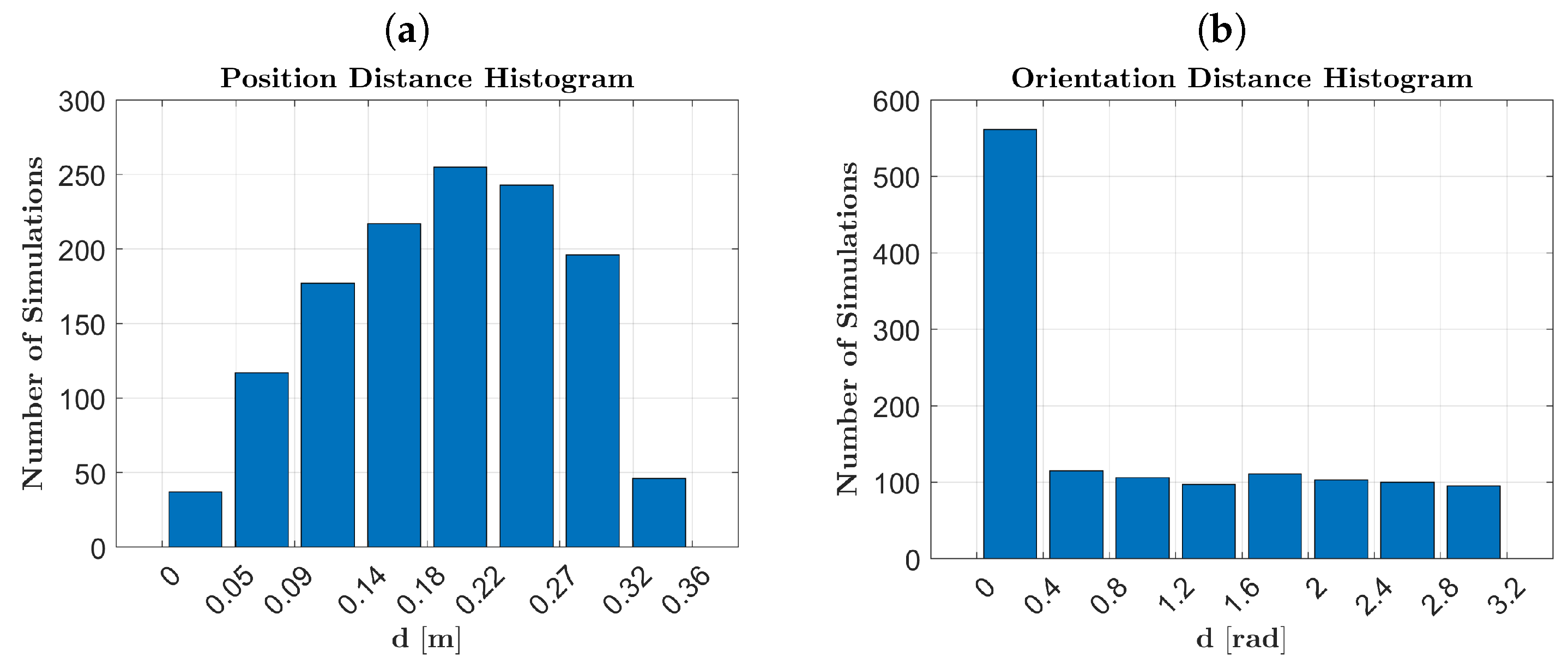
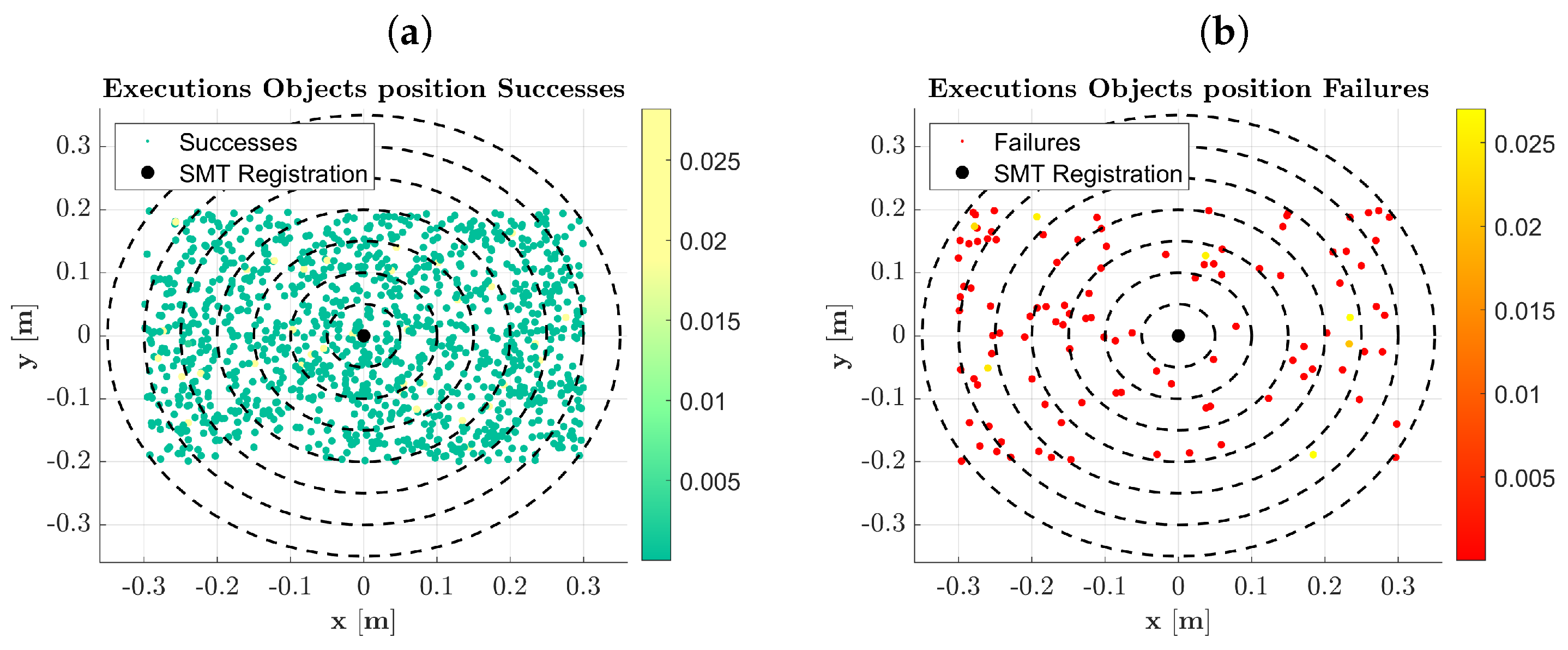
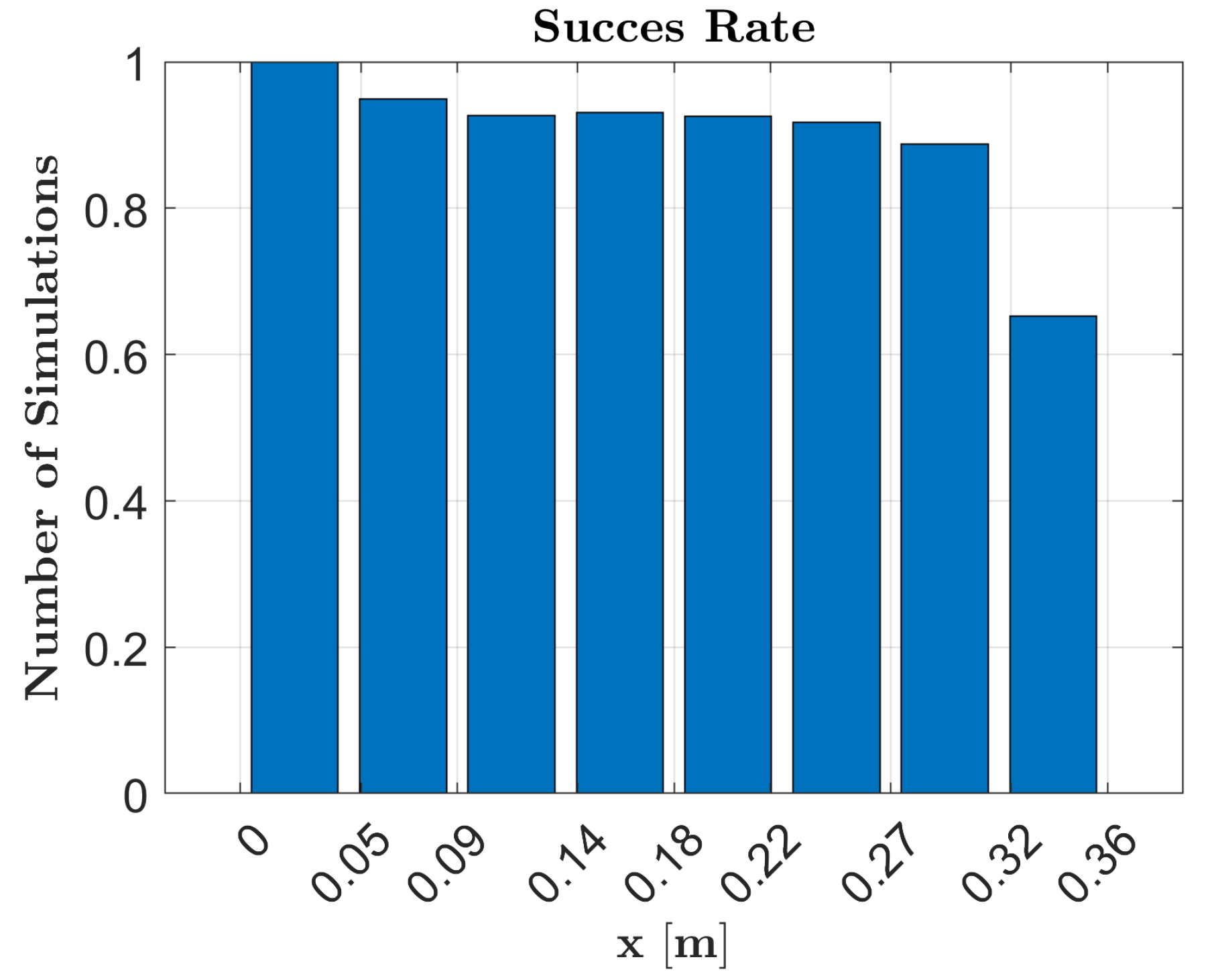
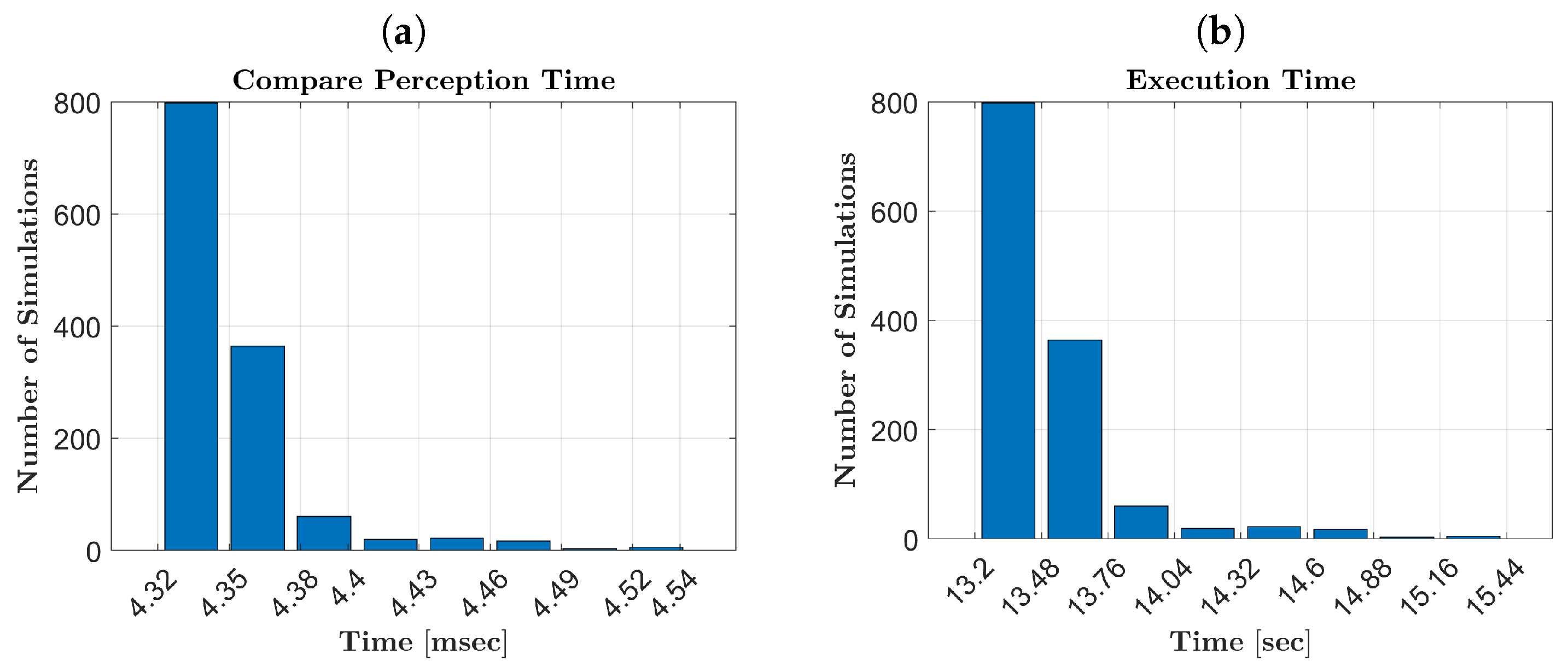
The validation in a pick-and-place simulation scenario demonstrated the robustness and repeatability of the framework, achieving a success rate of over 90%. Examining Figure 11, we observe a decreasing success rate as the object’s location moves further away from the SMT registration point. This decrease is attributed to the increased pose error estimation as objects are positioned near the camera’s field of view boundary. Additionally, from Figure 12a, we notice an increase in time for the vision system to recognize objects located farther away.

Figure 12a,b reveal that the average execution times are lower than the SMT registration time (15 s). This efficiency is achieved by the framework’s design, which eliminates waiting time when the user initiates or concludes SMT fragments. The variance in execution times is primarily due to the vision system’s need to compare incoming perceptions with stored ones to identify objects for grasping.

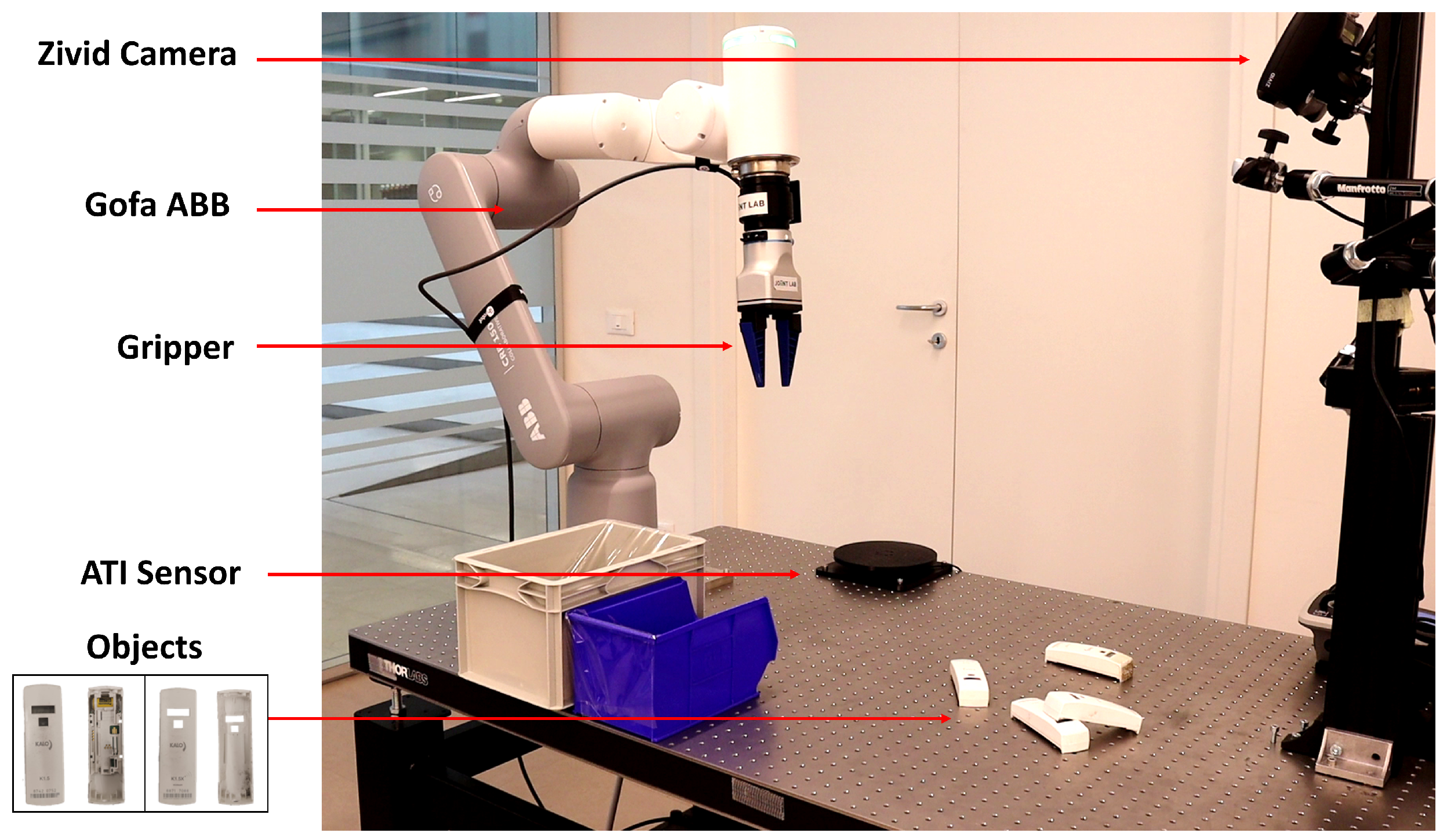
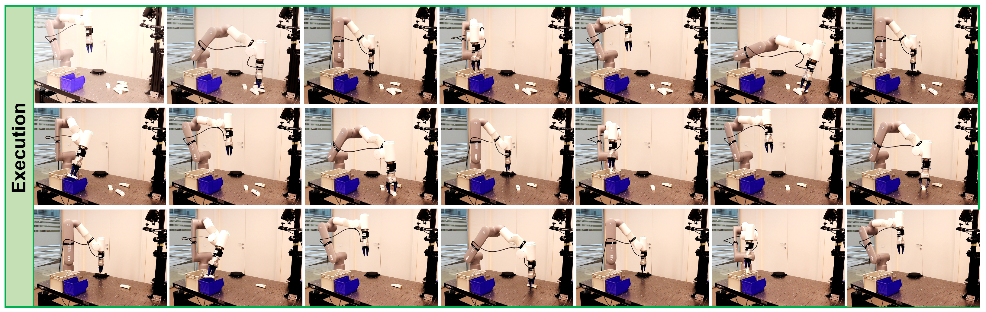
In our real experiments, we assessed the framework’s capabilities in managing and integrating diverse robotic systems and sensors. In the first real experiment, the system successfully extracted salient SMC perceptions from the camera and weight sensor, as well as merged the initial SMCs from each SMT. Thanks to the SMCs tree, the robot autonomously and efficiently sorted objects on the table. Employing identical parameters from the simulation, real-world manipulation achieved a 100% success rate in sorting the five objects. However, due to the limited number of tested objects, it is impossible to conclude on the statistical significance of that specific experiment. Nonetheless, the reported results and the experiment video contained in the multimedia file demonstrate the exemplary performance of the simulation-developed system in real-world applications.

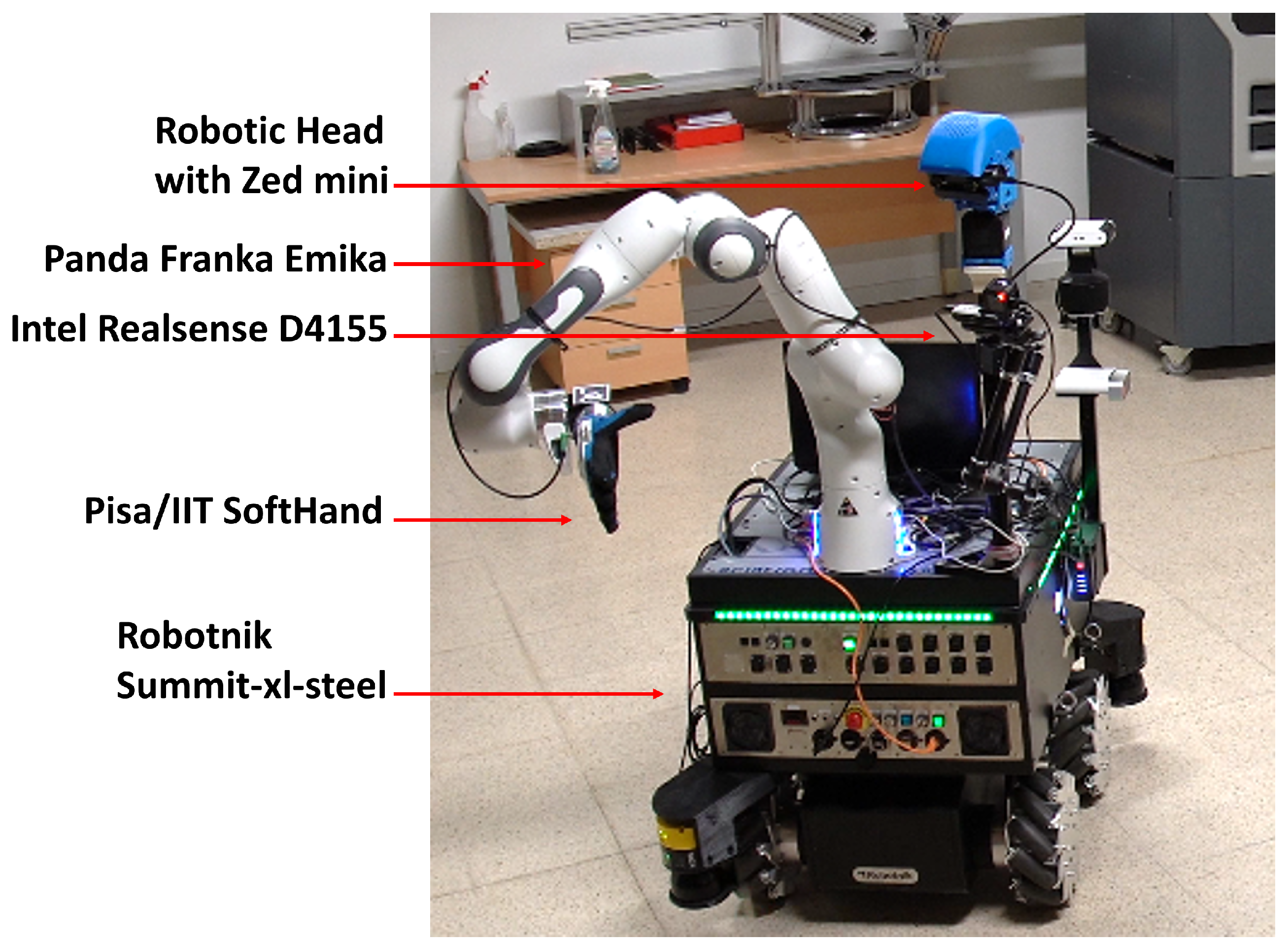
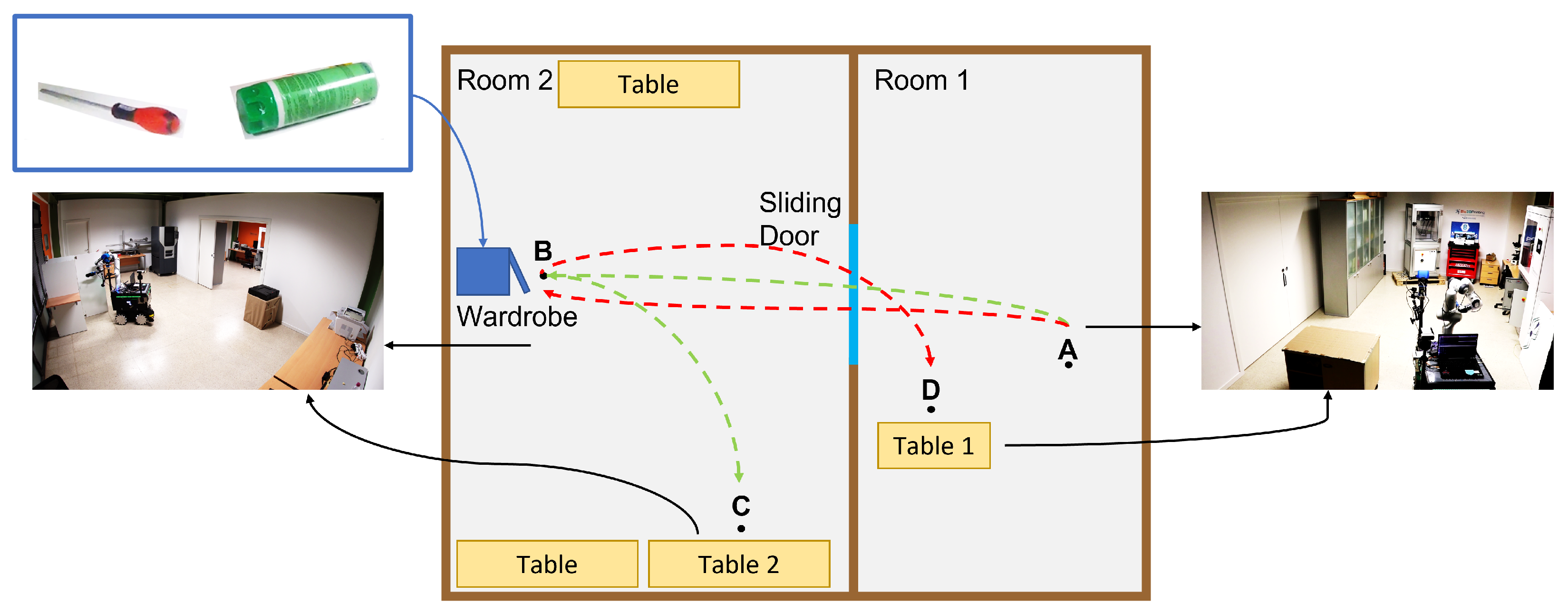
The framework’s architecture was thoughtfully designed to seamlessly transition between manipulation tasks and loco-manipulation ones, allowing us to evaluate the framework in combined tasks. The loco-manipulation experiment illustrated the framework’s proficiency in learning and managing combined SMTs, particularly in scenarios necessitating synchronization between manipulation and navigation—an accomplishment that traditional planners often struggle with. From the multimedia material depicting the autonomous executions, it becomes evident that the robot adeptly handled real-time changes in the wardrobe’s pose during execution. It demonstrated a remarkable ability to seamlessly adapt to the dynamic adjustments of the furniture, ensuring precise task execution even in the face of unexpected movements.

Affordances in SMCs-Tree

Building an SMC-Tree as described in Section 3.8 can provide the robot with an implicit representation of the affordances that exist in a given environment. Indeed, the different branches sprouting from similar scenarios (e.g., the vision of a bottle) could lead to the execution of actions linked to different affordances (e.g., fill-in the bottle, open the bottle-cap, pour the bottle content in a glass, etc.…). However, although we can link affordances to the branches that sprout from a given node, there is not a one-to-one correspondence between affordances and branches, as there could be more than one branch associated with the same affordance, and there could be affordances that are not explored by the tree at all.

Moreover, it is important that our SMC-based framework relies on the hypothesis that there exists some perception P of the environment that can be used to tell which is the right SMC branch to follow along the tree. Therefore, although one could imagine using variations of our approach to build a tree representing all the possible affordances of a given object by combining many SMTs (one for each affordance to learn), some affordances may manifest in Sensory-Motor Traces (SMTs) as a consequence of unobservable variables that exist solely in the operator’s intentions. When two identical situations differ only in their unmanifested intentions, it becomes challenging to capture and represent the information solely through SMTs. Consequently, one would need to explicitly express these intentions, perhaps through an additional operator command signal, to effectively account for the subtle distinctions in the tree and explore all possible affordances of a scenario.

7. Conclusions

In this work, we have presented a comprehensive framework for robot programming, centered around the acquisition of multiple Sensory-Motor Contingencies (SMCs) derived from human demonstrations. Our framework extends the fundamental concept of identifying pertinent perceptions within a given context, allowing us to detect salient phases within Sensory-Motor Traces (SMTs) and establish a sensor space metric. This metric empowers the agent to assess the robot’s interactions with the environment and recognize stored contingent SMTs in its memory. Moreover, we leveraged Learning from Demonstration techniques to abstract and generalize learned action patterns, thereby enhancing the adaptability of our system to diverse environmental conditions. Consequently, we extracted a comprehensive collection of SMCs, effectively encapsulating the intricate relationships between actions and sensory changes, organized in a tree structure based on historical observations and actions.

To validate our framework, we conducted an extensive set of numerical validation experiments, involving over a thousand pick-and-place tasks in both simulated and real-world settings. In the simulated validation, we achieved a success rate of 91.382%, demonstrating the efficacy of our framework in virtual environments. Conversely, in both real-world experiments, we attained a remarkable 100% success rate, underscoring the robustness and reliability of our system across physical applications. These experiments utilized both a manipulator and a mobile manipulator platform, showcasing the versatility and robustness of our system.

In future endeavors, we aim to further test our framework in various operating conditions and explore opportunities for integrating collaborative tasks across multiple robotic systems. Moreover, we plan to explore the representation of affordances within the framework of SMC trees, since we believe that this could enable agents to perceive and respond to a wider range of action possibilities presented by their environment.

8. Patents

The research showcased in this paper is encompassed by Patent Number WO2022175777A1.

References

1. Johansson, R.S.; Edin, B.B. Predictive feed-forward sensory control during grasping and manipulation in man. Biomed. Res. 1993, 14, 95–106. [Google Scholar]
2. Jacquey, L.; Baldassarre, G.; Santucci, V.G.; O’regan, J.K. Sensorimotor contingencies as a key drive of development: From babies to robots. Front. Neurorobot. 2019, 13, 98. [Google Scholar] [CrossRef] [PubMed]
3. Buhrmann, T.; Di Paolo, E.A.; Barandiaran, X. A dynamical systems account of sensorimotor contingencies. Front. Psychol. 2013, 4, 285. [Google Scholar] [CrossRef] [PubMed]
4. O’Regan, J.K.; Noë, A. What it is like to see: A sensorimotor theory of perceptual experience. Synthese 2001, 129, 79–103. [Google Scholar] [CrossRef]
5. Maye, A.; Engel, A.K. A discrete computational model of sensorimotor contingencies for object perception and control of behavior. In Proceedings of the 2011 IEEE International Conference on Robotics and Automation, IEEE, Shanghai, China, 3–13 May 2011; pp. 3810–3815. [Google Scholar]
6. Maye, A.; Engel, A.K. Using sensorimotor contingencies for prediction and action planning. In Proceedings of the From Animals to Animats 12: 12th International Conference on Simulation of Adaptive Behavior, SAB 2012, Odense, Denmark, 27–30 August 2012; Proceedings 12; Springer: Berlin/Heidelberg, Germany, 2012; pp. 106–116. [Google Scholar]
7. Hoffmann, M.; Schmidt, N.M.; Pfeifer, R.; Engel, A.K.; Maye, A. Using sensorimotor contingencies for terrain discrimination and adaptive walking behavior in the quadruped robot puppy. In Proceedings of the From Animals to Animats 12: 12th International Conference on Simulation of Adaptive Behavior, SAB 2012, Odense, Denmark, 27–30 August 2012; Proceedings 12; Springer: Berlin/Heidelberg, Germany, 2012; pp. 54–64. [Google Scholar]
8. Lübbert, A.; Göschl, F.; Krause, H.; Schneider, T.R.; Maye, A.; Engel, A.K. Socializing sensorimotor contingencies. Front. Hum. Neurosci. 2021, 15, 624610. [Google Scholar] [CrossRef]
9. Gibson, J.J. The Ecological Approach to Visual Perception: Classic Edition; Psychology Press: London, UK, 2014. [Google Scholar]
10. Maye, A.; Engel, A.K. Extending sensorimotor contingency theory: Prediction, planning, and action generation. Adapt. Behav. 2013, 21, 423–436. [Google Scholar] [CrossRef]
11. Ardón, P.; Pairet, È.; Lohan, K.S.; Ramamoorthy, S.; Petrick, R.P.A. Building Affordance Relations for Robotic Agents—A Review. arXiv 2021, arXiv:2105.06706. [Google Scholar]
12. Montesano, L.; Lopes, M.; Bernardino, A.; Santos-Victor, J. Modeling affordances using bayesian networks. In Proceedings of the 2007 IEEE/RSJ International Conference on Intelligent Robots and Systems, IEEE, San Diego, CA, USA, 29 October–2 November 2007; pp. 4102–4107. [Google Scholar]
13. Krüger, N.; Geib, C.; Piater, J.; Petrick, R.; Steedman, M.; Wörgötter, F.; Ude, A.; Asfour, T.; Kraft, D.; Omrčen, D.; et al. Object–action complexes: Grounded abstractions of sensory–motor processes. Robot. Auton. Syst. 2011, 59, 740–757. [Google Scholar] [CrossRef]
14. Dogar, M.R.; Ugur, E.; Sahin, E.; Cakmak, M. Using learned affordances for robotic behavior development. In Proceedings of the 2008 IEEE International Conference on Robotics and Automation, Pasadena, CA, USA, 19–23 May 2008; pp. 3802–3807. [Google Scholar] [CrossRef]
15. Ardón, P.; Pairet, È.; Lohan, K.S.; Ramamoorthy, S.; Petrick, R. Affordances in robotic tasks–a survey. arXiv 2020, arXiv:2004.07400. [Google Scholar]
16. Datteri, E.; Teti, G.; Laschi, C.; Tamburrini, G.; Dario, G.; Guglielmelli, E. Expected perception: An anticipation-based perception-action scheme in robots. In Proceedings of the 2003 IEEE/RSJ International Conference on Intelligent Robots and Systems (IROS 2003) (Cat. No.03CH37453), Las Vegas, NV, USA, 27–31 October 2003; Volume 1, pp. 934–939. [Google Scholar] [CrossRef]
17. Qi, J.; Ran, G.; Wang, B.; Liu, J.; Ma, W.; Zhou, P.; Navarro-Alarcon, D. Adaptive shape servoing of elastic rods using parameterized regression features and auto-tuning motion controls. IEEE Robot. Autom. Lett. 2023, 9, 1428–1435. [Google Scholar] [CrossRef]
18. Yang, C.; Zhou, P.; Qi, J. Integrating visual foundation models for enhanced robot manipulation and motion planning: A layered approach. arXiv 2023, arXiv:2309.11244. [Google Scholar]
19. Kober, J.; Bagnell, J.A.; Peters, J. Reinforcement learning in robotics: A survey. Int. J. Robot. Res. 2013, 32, 1238–1274. [Google Scholar] [CrossRef]
20. Ghadirzadeh, A.; Bütepage, J.; Maki, A.; Kragic, D.; Björkman, M. A sensorimotor reinforcement learning framework for physical Human-Robot Interaction. In Proceedings of the 2016 IEEE/RSJ International Conference on Intelligent Robots and Systems (IROS), Daejeon, Republic of Korea, 9–14 October 2016; pp. 2682–2688. [Google Scholar] [CrossRef]
21. Hay, N.; Stark, M.; Schlegel, A.; Wendelken, C.; Park, D.; Purdy, E.; Silver, T.; Phoenix, D.S.; George, D. Behavior Is Everything: Towards Representing Concepts with Sensorimotor Contingencies. Proc. AAAI Conf. Artif. Intell. 2018, 32. [Google Scholar] [CrossRef]
22. Dulac-Arnold, G.; Levine, N.; Mankowitz, D.J.; Li, J.; Paduraru, C.; Gowal, S.; Hester, T. Challenges of real-world reinforcement learning: Definitions, benchmarks and analysis. Mach. Learn. 2021, 110, 2419–2468. [Google Scholar] [CrossRef]
23. Maye, A.; Trendafilov, D.; Polani, D.; Engel, A. A visual attention mechanism for autonomous robots controlled by sensorimotor contingencies. In Proceedings of the IROS 2015 Workshop on Sensorimotor Contingencies For Robotics, Hamburg, Germany, 2 October 2015. [Google Scholar]
24. Ravichandar, H.; Polydoros, A.S.; Chernova, S.; Billard, A. Recent advances in robot learning from demonstration. Annu. Rev. Control. Robot. Auton. Syst. 2020, 3, 297–330. [Google Scholar] [CrossRef]
25. Correia, A.; Alexandre, L.A. A Survey of Demonstration Learning. arXiv 2023, arXiv:2303.11191. [Google Scholar]
26. Li, J.; Wang, J.; Wang, S.; Yang, C. Human–robot skill transmission for mobile robot via learning by demonstration. Neural Comput. Appl. 2021, 35, 23441–23451. [Google Scholar] [CrossRef]
27. Zhao, J.; Giammarino, A.; Lamon, E.; Gandarias, J.M.; De Momi, E.; Ajoudani, A. A Hybrid Learning and Optimization Framework to Achieve Physically Interactive Tasks With Mobile Manipulators. IEEE Robot. Autom. Lett. 2022, 7, 8036–8043. [Google Scholar] [CrossRef]
28. Somers, T.; Hollinger, G.A. Human–robot planning and learning for marine data collection. Auton. Robot. 2016, 40, 1123–1137. [Google Scholar] [CrossRef]
29. Zeng, A.; Florence, P.; Tompson, J.; Welker, S.; Chien, J.; Attarian, M.; Armstrong, T.; Krasin, I.; Duong, D.; Sindhwani, V.; et al. Transporter networks: Rearranging the visual world for robotic manipulation. In Proceedings of the Conference on Robot Learning, PMLR, London, UK, 8–11 November 2021; pp. 726–747. [Google Scholar]
30. Zhang, T.; McCarthy, Z.; Jow, O.; Lee, D.; Chen, X.; Goldberg, K.; Abbeel, P. Deep imitation learning for complex manipulation tasks from virtual reality teleoperation. In Proceedings of the 2018 IEEE International Conference on Robotics and Automation (ICRA), IEEE, Brisbane, Australia, 21–25 May 2018; pp. 1–8. [Google Scholar]
31. Zhu, Y.; Wang, Z.; Merel, J.; Rusu, A.; Erez, T.; Cabi, S.; Tunyasuvunakool, S.; Kramár, J.; Hadsell, R.; de Freitas, N.; et al. Reinforcement and imitation learning for diverse visuomotor skills. arXiv 2018, arXiv:1802.09564. [Google Scholar]
32. Li, Y.; Song, J.; Ermon, S. Infogail: Interpretable imitation learning from visual demonstrations. In Advances in Neural Information Processing Systems 30 (NIPS 2017), Proceedings of the 31st Conference on Neural Information Processing Systems (NIPS 2017), Long Beach, CA, USA, 4–9 December 2017; Neural Inforamation Processing Systems: San Diego, CA, USA, 2017; Volume 30. [Google Scholar]
33. Pan, Y.; Cheng, C.A.; Saigol, K.; Lee, K.; Yan, X.; Theodorou, E.; Boots, B. Agile autonomous driving using end-to-end deep imitation learning. arXiv 2017, arXiv:1709.07174. [Google Scholar]
34. Loquercio, A.; Maqueda, A.I.; Del-Blanco, C.R.; Scaramuzza, D. Dronet: Learning to fly by driving. IEEE Robot. Autom. Lett. 2018, 3, 1088–1095. [Google Scholar] [CrossRef]
35. Calandra, R.; Gopalan, N.; Seyfarth, A.; Peters, J.; Deisenroth, M.P. Bayesian Gait Optimization for Bipedal Locomotion. In Proceedings of the LION, Learning and Intelligent Optimization: 8th International Conference, Lion 8, Gainesville, FL, USA, 16–21 February 2014. [Google Scholar]
36. Gopalan, N.; Moorman, N.; Natarajan, M.; Gombolay, M. Negative Result for Learning from Demonstration: Challenges for End-Users Teaching Robots with Task and Motion Planning Abstractions. In Proceedings of the Robotics: Science and Systems (RSS), New York, NY, USA, 27 June–1 July 2022. [Google Scholar]
37. Maye, A.; Engel, A.K. Context-dependent dynamic weighting of information from multiple sensory modalities. In Proceedings of the 2013 IEEE/RSJ International Conference on Intelligent Robots and Systems, Tokyo, Japan, 3–7 November 2013; pp. 2812–2818. [Google Scholar] [CrossRef]
38. O’regan, J.K.; Noë, A. A sensorimotor account of vision and visual consciousness. Behav. Brain Sci. 2001, 24, 939–973. [Google Scholar] [CrossRef] [PubMed]
39. Ijspeert, A.J.; Nakanishi, J.; Hoffmann, H.; Pastor, P.; Schaal, S. Dynamical movement primitives: Learning attractor models for motor behaviors. Neural Comput. 2013, 25, 328–373. [Google Scholar] [CrossRef] [PubMed]
40. Sinaga, K.P.; Yang, M.S. Unsupervised K-means clustering algorithm. IEEE Access 2020, 8, 80716–80727. [Google Scholar] [CrossRef]
41. Brugnara, F.; Falavigna, D.; Omologo, M. Automatic segmentation and labeling of speech based on hidden Markov models. Speech Commun. 1993, 12, 357–370. [Google Scholar] [CrossRef]
42. Zhang, H.; Han, X.; Zhang, W.; Zhou, W. Complex sequential tasks learning with Bayesian inference and Gaussian mixture model. In Proceedings of the 2018 IEEE International Conference on Robotics and Biomimetics (ROBIO), IEEE, Kuala Lumpur, Malaysia, 12–15 December 2018; pp. 1927–1934. [Google Scholar]
43. Escudero-Rodrigo, D.; Alquezar, R. Distance-based kernels for dynamical movement primitives. In Artificial Intelligence Research and Development; IOS Press: Amsterdam, The Netherlands, 2015; pp. 133–142. [Google Scholar]
44. Koenig, N.; Howard, A. Design and use paradigms for Gazebo, an open-source multi-robot simulator. In Proceedings of the 2004 IEEE/RSJ International Conference on Intelligent Robots and Systems (IROS) (IEEE Cat. No.04CH37566), Sendai, Japan, 28 September–2 October 2004; Volume 3, pp. 2149–2154. [Google Scholar] [CrossRef]
45. Bhattacharyya, A. On a Measure of Divergence between Two Multinomial Populations. Sankhya Indian J. Stat. 1946, 7, 401–406. [Google Scholar]
46. Ajoudani, A. Teleimpedance: Teleoperation with impedance regulation using a body-machine interface. In Transferring Human Impedance Regulation Skills to Robots; Springer: Berlin/Heidelberg, Germany, 2016; pp. 19–31. [Google Scholar]
47. Catalano, M.G.; Grioli, G.; Farnioli, E.; Serio, A.; Piazza, C.; Bicchi, A. Adaptive synergies for the design and control of the Pisa/IIT SoftHand. Int. J. Robot. Res. 2014, 33, 768–782. [Google Scholar] [CrossRef]
Figure 1. Temporal Causality Relations in Sensori-Motor Trace (SMT): in each SMT, the sensorimoror interactions are composed of a perception that causes an action (black arrow) and a perception that is the consequence of an action (red arrow).
Robotics 13 00058 g001
Figure 2. Desired representation that models sensorimotor interactions.
Robotics 13 00058 g002
Figure 3. Temporal saliency extraction: For each Sensori-Motor Trace T i , the temporal saliency extraction results in a sequence of SMT fragments recorded two streaming of data: the actions commanded to the robot A i , j and the perceptions registered by the robot P i , j .
Robotics 13 00058 g003
Figure 4. SMCs-tree: the SMCs are extracted to produce a SMCs-tree where the nodes represent the decision points where the temporal saliency was extracted, and each oriented edge connecting two nodes i and j is a SMC composed by a pair of salient perceptions-action.
Robotics 13 00058 g004
Figure 5. Multiple Localized Perception Example. SMTs Registration: from the same initial configuration two SMTs are registered. In the first SMT T 1 (a,b), the robot detects an orange cube and a green cylinder, then, it grasps the orange cube (a) and puts it on the green cylinder (b). In the second SMT T 2 (d,e), the robot perceives a grey pyramid and a yellow cylinder, grasps the pyramid (e) and puts it on the yellow cylinder. SMCs Extraction: in each SMT the robot learns the salient perceptions (cluster color of the object nearest to the E.E.) and the associated salient action highlighted, respectively, in orange and yellow in the figures. After extracting the SMCs from the first SMT, the robot builds the SMCs tree in (c), while, after the second SMT the final SMCs tree is in (f).
Robotics 13 00058 g005
Figure 6. Robotic Mobile Base Merging Branches Example. SMTs Registration: from the same initial configuration two SMTs are registered. In the first SMT T 1 (a,b), the robot moves to x 1 , 1 (a) and, after seeing a green arrow, reaches its final configuration x 1 , 2 (b). In the second SMT T 2 (d,e), the robot moves to x 2 , 1 (d) and, after seeing a yellow arrow, reaches its final configuration x 2 , 2 (e). SMCs Extraction: in each SMT the robot learns the salient perceptions (color histogram and lidar point cloud) and the associated action highlighted, respectively, in orange and yellow in the figures. After extracting the SMCs from the first SMT, the robot builds the SMCs tree in (c), while, after the second SMT the final SMCs tree is in (f). Since the first subtasks of the two SMTs are contingent, they are merged by the SMCs tree building process.
Robotics 13 00058 g006
Figure 7. Robotic Arm Merging Branches Example. SMTs Registration: from the same initial configuration two SMTs are registered. In the first SMT T 1 (ac), the robot perceives and grasps an orange cube (a), weighs it (b) and finally puts it down to his right (c). In the second SMT T 2 (eg), the robot perceives and grasps the same orange cube (e), weight it (f), and finally puts it on top to his right (g). SMCs Extraction: in each SMT the robot learns the salient perceptions (object cluster color and weight) and the associated action highlighted, respectively, in orange and yellow in the figures. After extracting the SMCs from the first SMT, the robot builds the SMCs tree in (c), while, after the second SMT the final SMCs tree is in (f). Since the first two subtasks of the two SMTs are contingent, they are merged by the SMCs tree building process.
Robotics 13 00058 g007
Figure 8. SMCs tree in the Pick-and-Place experiment.
Robotics 13 00058 g008
Figure 9. Pose distances histograms with respect to the SMT registration pose: (a) position and (b) orientation distance histogram of each object during the execution with respect to the SMT registration perceived object.
Robotics 13 00058 g009
Figure 10. Objects Positions: in the figures there are all the objects initial position (x,y) in each execution. The marker color depends on the objects height (0.0 m = on the table). In black, there is the object initial position in the registration phase. Figure (a) depicts all the successes, while (b) presents all the failures. Finally, the dotted circles correspond to the intervals in Figure 11.
Robotics 13 00058 g010
Figure 11. Success Rate: the success rate related to the distance from the initial position of the object during registration.
Robotics 13 00058 g011
Figure 12. Figure (a) shows the time taken by the vision system to recognize the object to be grasped in each execution; (b) shows the duration of each pick-and-place task execution.
Robotics 13 00058 g012
Figure 13. Manipulation Task Setup: the manipulation task setup includes a Gofa ABB 7 DoFs arms equipped with a two fingers gripper as EE, an Inustrial Zivid Camera and an ATI sensor to perceive and weigh the Heat-counters on the table.
Robotics 13 00058 g013
Figure 14. SMCs tree in the Real Manipulation Experiments: The system registered two different SMTs. In the first one, the user took a heater-counter without electronics, weighed it, and placed it in the blue box; while in the second, he carried out the same procedure but with a heater-counter with electronics and, having a different weight, placed it in the white box. Since the first two SMCs fragments of each SMT have the same perceptions and actions (are contingent), they were merged during the SMCs tree building phase.
Robotics 13 00058 g014
Figure 15. Execution phase in the Real Manipulation Experiments: all the heat-counters were sorted correctly according to their weight.
Robotics 13 00058 g015
Figure 16. Mobile Manipulator Robot System: the mobile manipulator system includes a Robotnik Summit-xl-steel platform, a Panda Franka Emika robot with 7 Degrees of Freedom (DoFs) arms, featuring a Pisa/IIT SoftHand as End Effector (EE), a two-degree-of-freedom robotic head equipped with a Zed mini camera and an Intel Realsense D4155 camera to perceive the environment.
Robotics 13 00058 g016
Figure 17. Real Experiments Environment Scheme: In the first SMT registration, the robot traveled the green route: starting from point A, it opened a sliding door, took an object from the wardrobe in B, and placed it on a table at the final point C. Instead, in the second registration, it traveled the red path by opening the same sliding door, taking a different object in the wardrobe in B, and placing it on a table at the final point D.
Robotics 13 00058 g017
Figure 18. SMCs tree in the Real Loco-manipulation Experiments: The system registered two different SMTs. In the first SMT, the user controlled the robot to reach a sliding door, open it, navigate to a wardrobe, open it, take a green can, and place it on a table. Instead, in the second SMT, the human operator controlled the robot to open the same sliding door, take a different object in the wardrobe, and place it on a different table. The SMCs tree building process merged all the SMCs fragments of the two SMTs up to the SMC in which the robot grasped different objects.
Robotics 13 00058 g018
Disclaimer/Publisher’s Note: The statements, opinions and data contained in all publications are solely those of the individual author(s) and contributor(s) and not of MDPI and/or the editor(s). MDPI and/or the editor(s) disclaim responsibility for any injury to people or property resulting from any ideas, methods, instructions or products referred to in the content.