Motion Planning of Differentially Flat Planar Underactuated Robots

Abstract

Differential flat underactuated robots have fewer actuators than degrees of freedom (DOFs). This characteristic makes it possible to design light and cost-effective robots with great dexterity. The primary challenge associated with these robots lies in effectively controlling the passive joint, in particular, when collisions with obstacles in the workspace have to be avoided. Most of the previous research focused on point-to-point motions without any control on the actual robot trajectory. In this work, a new method is presented to plan trajectories that include one or more via points. In this way, the underactuated robot can avoid the obstacles in the workspace, similarly to traditional fully actuated robots. First, a trajectory planning strategy is analytically described; then, numerical results are presented. The numerical results show the effects of the via points and of the order of the polynomials adopted to define the motion laws. In addition, experimental tests performed on a two-DOF underactuated robot are presented, and their results validate the proposed method.

1. Introduction

Most mechanical systems used in engineering applications have one controlled actuator for each degree of freedom (DOF) or have no actuator and are driven by external forces that cannot be controlled. The first class includes machine tools and robots, and the second class includes vibrating systems excited by base motion, unbalance, wind, and other physical phenomena. Underactuated mechanical systems are less common and have more DOFs than actuators [1,2]. In recent years, the interest in underactuated systems has increased in the field of robotics [3,4,5] and legged locomotion [6,7].

Underactuated robots are a promising solution for applications requiring an increase in dexterity and, at the same time, decreases in the cost, encumbrance, and weight of the robot [8,9]. In this class of robots, one or more joints of the kinematic chain are not driven by motors but are equipped with springs. From the mathematical point of view, underactuated robots are characterized by the presence of nonholonomic second-order constraints that represent the dynamics of the passive joints [10,11]. The main problem of underactuated robots is control, since the passive joints have to be indirectly controlled by the motors of the commanded joints.

A great deal of research has been carried out on the planning of point-to-point motions exploiting differential flatness properties [12,13,14,15]. In order to achieve differential flatness, the last links of the robot must have a particular mass distribution with the center of mass (COM) of some links lying on joint axes [12,16]. This property simplifies the last rows of the mass matrix and leads to the cancellation of some gravity, Coriolis, and centrifugal torques, and the nonholonomic constraint becomes integrable [10]. When a mechanical system— in particular, a robot—is differentially flat, a set of variables can be defined to express the state variables, which are called flat variables [8,12]. The number of flat variables is equal to the number of actuated DOFs. The relationship between state variables and flat variables is called diffeomorphism [17]. Actually, the diffeomorphism transforms a system of second-order differential equations into a reduced set of higher-order equations.

In robotic applications, often there are obstacles in the workspace. The possibility of avoiding an obstacle can be strongly increased by not only specifying the initial and final configurations but also introducing one or more via points that modify the trajectory of the end effector near the obstacle [18,19]. However, to the best of the authors’ knowledge, the trajectory planning for differentially flat underactuated robots has never been performed including via points. In fact, many aspects of the control of differentially flat robots have been studied over the years, but only point-to-point motions have been considered [13,20], leaving a research gap to be filled. It is worth noticing that trajectory planning with via points for underactuated robots has been studied before (e.g., for mobile robots [21,22]), but not in the case of differentially flat robots. For this reason, this paper deals with motion planning of differentially flat underactuated robots with one or more via points.

The main contribution of the paper is the development and validation of a general trajectory planning algorithm in the space of flat variables. It is worth noting that for this class of robots, trajectory planning is not a purely kinematic problem, but it is influenced by dynamics, since the last joint is not directly driven.

The paper is organized as follows. In Section 2, the conditions of differential flatness are stated, and the equations of motion of the planar underactuated robot are presented and their special features are discussed. Section 3 discusses the main point of the research and deals with path planning considering one or more via points. In Section 4, numerical results are presented and discussed. An experimental validation of the method is presented in Section 5. Finally, conclusions and possible future developments are presented in Section 6.

2. Mathematical Model of the Underactuated Robot

In the framework of this research, the analyzed robots are differentially flat since they comply with the requirements of the theory of differential flatness [8] as follows:

• The last link center of mass (n) lies on the axis of the n-th joint;
• The overall center of mass of the links n and $n-1$ lies on the axis of the $(n-1)$-th joint.

Such requirements remain valid for the last j links (i.e., $n,n-1,\dots ,n-j+1$), where $j-1$ is the number of passive joints. As a result, the center of mass of the last j links lies on the $(n-j+1)$-th joint axis, and the final j links are considered “fully balanced”.

To achieve controllability of the passive joints, a torsional spring is placed on the last $j-1$ joints.

This work focuses solely on a single passive joint; therefore, $j=2$. Therefore, only the joints n and $n-1$ are fully balanced.

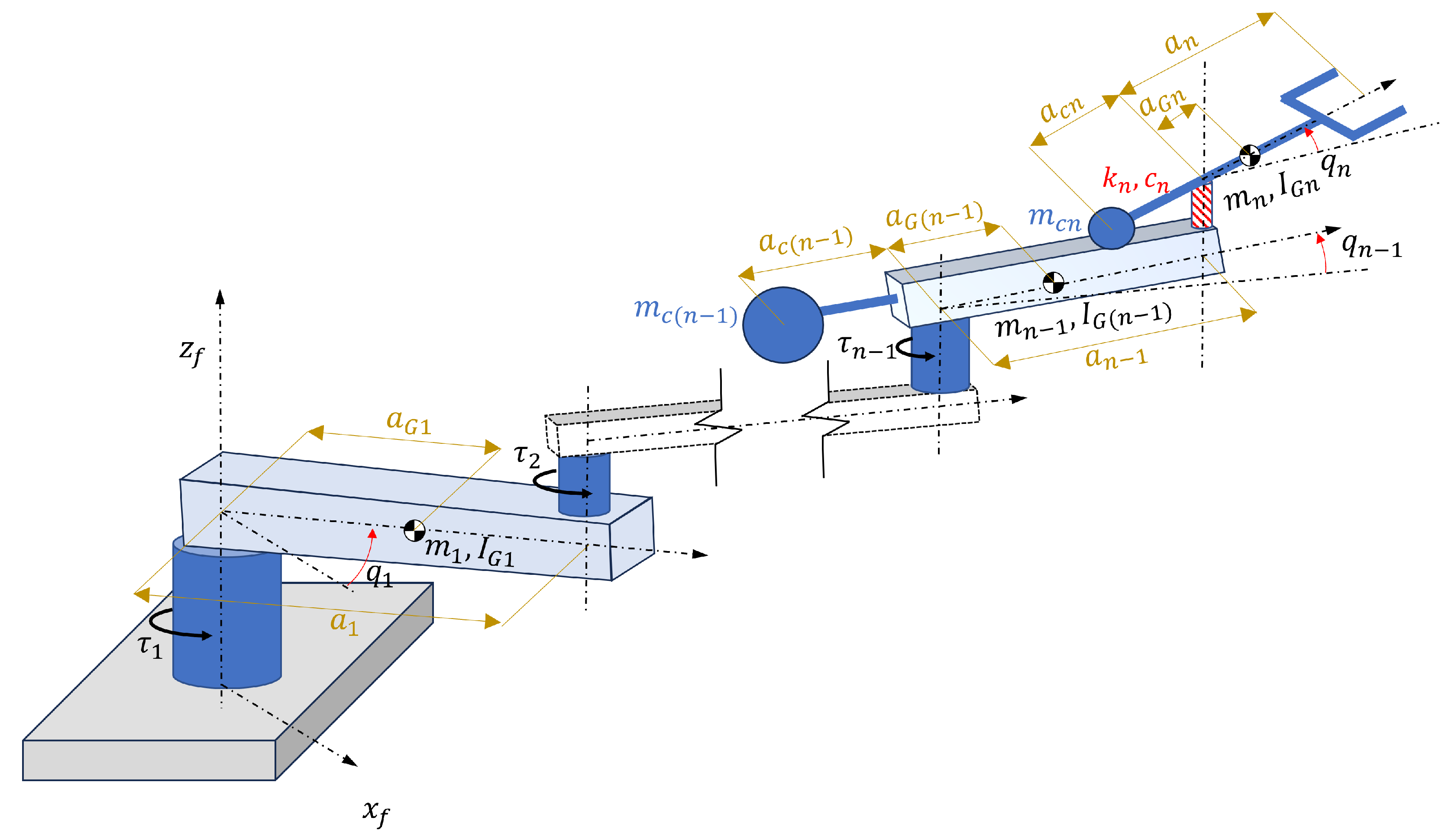
The scheme of the robot is depicted in Figure 1, in which for each i-th link, $q_i$ is the joint angle, $a_i$ is the link length, $a_{Gi}$ is the position of the center of mass with respect to the joint axis, and $m_i$ and $I_{Gi}$ are the mass and the moment of inertia about the center of mass, respectively. In the fully balanced links, $a_{ci}$ is the distance of the balancing mass $m_{ci}$ from joint i. At the passive joints, the torsional spring has stiffness $k_i$. A viscous damper with coefficient $c_i$ is included to introduce dissipative phenomena in the model. Neither elastic nor dissipative phenomena are included in the actuated joints because it is assumed that the control system of the actuated joints compensates for such effects.

The equations of motion of the planar robot can be obtained using Lagrange’s method. The system of equations of motion can be expressed in matrix form as follows [15]:

$$\begin{array}{c}{\mathit{M}}_n\left(\mathit{q}\right)\ddot{\mathit{q}}+{\mathit{C}}_n\dot{\mathit{q}}+{\mathit{K}}_n\mathit{q}+\mathit{b}(\mathit{q},\dot{\mathit{q}})+\mathit{g}\left(\mathit{q}\right)=\tau \\ {\mathit{M}}_n\left(\mathit{q}\right)\left[\begin{array}{c}{\ddot{q}}_1\\ {\ddot{q}}_2\\ ⋮\\ {\ddot{q}}_{n-2}\\ {\ddot{q}}_{n-1}\\ {\ddot{q}}_n\end{array}\right]+{\mathit{C}}_n\left[\begin{array}{c}{\dot{q}}_1\\ {\dot{q}}_2\\ ⋮\\ {\dot{q}}_{n-2}\\ {\dot{q}}_{n-1}\\ {\dot{q}}_n\end{array}\right]+{\mathit{K}}_n\left[\begin{array}{c}{q}_1\\ q_2\\ ⋮\\ q_{n-2}\\ q_{n-1}\\ q_n\end{array}\right]+\left[\begin{array}{c}{b}_1(\mathit{q},\dot{\mathit{q}})\\ b_2(\mathit{q},\dot{\mathit{q}})\\ ⋮\\ b_{n-2}(\mathit{q},\dot{\mathit{q}})\\ 0\\ 0\end{array}\right]+\left[\begin{array}{c}{g}_1\left(\mathit{q}\right)\\ g_2\left(\mathit{q}\right)\\ ⋮\\ g_{n-2}\left(\mathit{q}\right)\\ 0\\ 0\end{array}\right]=\left[\begin{array}{c}{\tau }_1\\ {\tau }_2\\ ⋮\\ {\tau }_{n-2}\\ {\tau }_{n-1}\\ 0\end{array}\right]\end{array}$$

(1)

where ${\mathit{M}}_n\left(\mathit{q}\right)$ is the mass matrix; matrices ${\mathit{C}}_n$ and ${\mathit{K}}_n$ contain the joint damping and stiffness terms, respectively; vector $\mathit{b}(\mathit{q},\dot{\mathit{q}})$ contains the Coriolis and centrifugal terms; vector $\mathit{g}\left(\mathit{q}\right)$ contains the gravitational terms; and vector $\tau$ contains the motor torques. The following three features of the system of Equation (1) are worth noting:

• There are neither gravitational nor Coriolis-centrifugal torques on the last joints because the last two links are fully balanced (the last two elements of vectors $\mathit{b}(\mathit{q},\dot{\mathit{q}})$ and $\mathit{g}\left(\mathit{q}\right)$ are null);
• The last element of $\tau$ is null because there is no motor on the last joint (i.e., a passive joint);
• Matrices ${\mathit{C}}_n$ and ${\mathit{K}}_n$ are entirely null except the last bottom-right element, in which there are the torsional stiffness ($k_n$) and damping coefficient ($c_n$) of the passive joint; this happens because neither elastic nor dissipative phenomena are included in the actuated joints.

Matrix ${\mathit{M}}_n\left(\mathit{q}\right)$ is configuration-dependent. However, since the robot satisfies the conditions of differential flatness, the last $[n-1,n]$ rows and columns of the matrix are constant:

$${\mathit{M}}_n\left(\mathit{q}\right)=\left[\begin{array}{ccccc}& & & I_{n-1}^{*}& I_n^{*}\\ & & & I_{n-1}^{*}& I_n^{*}\\ & \multicolumn{3}{c}{{\mathit{I}}_{(n-2)\times (n-2)}^{*}\left(\mathit{q}\right)}& & ⋮& ⋮\\ & & & I_{n-1}^{*}& I_n^{*}\\ I_{n-1}^{*}& \cdots & I_{n-1}^{*}& I_{n-1}^{*}& I_n^{*}\\ I_n^{*}& \cdots & I_n^{*}& I_n^{*}& I_n^{*}\end{array}\right]$$

(2)

Addtionally, only the submatrix ${\mathit{I}}_{(n-2)\times (n-2)}^{*}\left(\mathit{q}\right)$ depends on the robot configuration. $I_{n-1}^{*}$ and $I_n^{*}$ are the moments of inertia reduced to joints $n-1$ and n, respectively.

The theory of differential flatness is then used to define a reduced set of variables $\mathit{y}$ (called flat variables), equal to the number of actuators [23]. For a planar robot equipped with only one passive joint, the flat variables are defined as follows [15]:

$$\begin{array}{c}{y}_1={\displaystyle \sum _{i=1}^n}{q}_i\\ y_i=q_{i-1}\mathrm{with}i=2,3,\cdots ,n-1\end{array}$$

(3)

The flat variables are used to manipulate Equation (1), performing a diffeomorphism that maps the joint values into the flat variables, i.e., $\mathit{q}\in {\mathbb{R}}^n\mapsto \mathit{y}\in {\mathbb{R}}^{n-1}$.

The last row of Equation (1) becomes

$$I_n^{*}\left({\ddot{q}}_1+{\ddot{q}}_2+\cdots +{\ddot{q}}_{n-1}+{\ddot{q}}_n\right)+c_n{\dot{q}}_n+k_n{q}_n=0$$

(4)

which can be rewritten through the flat variable:

$$I_n^{*}{\dot{y}}_1+c_n{\dot{q}}_n+k_n{q}_n=0$$

(5)

This equation is linear since the inertia term $I_n^{*}$ is constant. As a result, the Laplace transform can be calculated [15]:

$$I_n^{*}s{Y}_1\left(s\right)+(c_{n}s+k_n)Q_n\left(s\right)=0$$

(6)

From this equation, the last joint rotation can be related to the flat variable:

$$Q_n\left(s\right)=-\frac{I_n^{*}}{c_{n}s+k_n}{s}^2{Y}_1\left(s\right)$$

(7)

Collecting the torsion spring stiffness $k_n$, the right term of the equation can be rearranged as

$$Q_n\left(s\right)=-\frac{I_n^{*}}{k_n}{\left(1+\frac{c_n}{k_n}s\right)}^{-1}{s}^2{Y}_1\left(s\right)$$

(8)

If low-friction bearings are used, the torsion spring stiffness is much larger than the damping coefficient $c_n$. Hence, using the first-order Taylor expansion, the term ${(1+c_n/k_{n}s)}^{-1}$ can be simplified, yielding the following:

$$Q_n\left(s\right)=-\frac{I_n^{*}}{k_n}\left(1-\frac{c_n}{k_n}s\right)s^2{Y}_1\left(s\right)=-\frac{I_n^{*}}{k_n}{s}^2{Y}_1\left(s\right)+\frac{I_n^{*}{c}_n}{k_n^2}{s}^3{Y}_1\left(s\right)$$

(9)

Finally, the passive joint position can be expressed as a function of time using the inverse Laplace transform, in which the initial conditions are null:

$$q_n\left(t\right)=-\frac{I_n^{*}}{k_n}{\ddot{y}}_1\left(t\right)+\frac{I_n^{*}{c}_n}{k_n^2}{y}_1^{\left(3\right)}\left(t\right)$$

(10)

It is worth noting that Equation (10) is more complex than the one usually found in the literature. Actually, many papers (e.g., [24,25]) simplify the system by neglecting damping (thus, $c_n=0$) so that $q_n$ is related only to the second derivative of $y_1$ rather than to a combination of ${\ddot{y}}_1$ and $y_1^{\left(3\right)}$. For this reason, the following sections will deal with trajectory planning for robots with both damped and undamped passive joint.

The dynamic model of Equation (1) contains joint accelerations. Hence, Equation (10) must be derived twice to obtain the passive joint acceleration, which depends on the flat variable:

$${\ddot{q}}_n\left(t\right)=-\frac{I_n^{*}}{k_n}{y}_1^{\left(4\right)}\left(t\right)+\frac{I_n^{*}{c}_n}{k_n^2}{y}_1^{\left(5\right)}\left(t\right)$$

(11)

Joint rotations $q_i\left(t\right)$ should be twice continuously differentiable ($C^2$) to avoid vibratory phenomena. As a result, Equation (11) yields that $y_1\left(t\right)$ must be continuously differentiable five times ($C^5$). The other flat variables ($y_2,\dots ,y_{n-1}$) are equal to the actuated joint values; hence, to avoid vibratory phenomena, these flat variables must be twice continuously differentiable ($C^2$).

3. Trajectory Planning

The typical trajectory planning of differentially flat underactuated robots considers only point-to-point movements and is performed in the space of flat variables. These movements provide fixed initial and final conditions for joint positions and their derivatives. The conditions for joint positions are the joint angles required to complete the task, apart from the passive joints, whose angles are set to zero to ensure the static equilibrium of the torsional spring. The conditions for the joint variable derivatives are null values at the beginning and at the end of the motion.

In trajectory planning with via points, the trajectories of fully actuated robots are usually planned in the joint space so that the via points are reached by the robot in specific configurations (i.e., joint variables), while the derivatives of joint variables are typically different from zero. Even if joint velocities and accelerations can be imposed, the continuity of joint variable derivatives is more important than the specific values. As a result, the conditions in the via points are limited to the joint positions and the continuity of joint variable derivatives. (please note that trajectory planning can also be performed in the Cartesian space by choosing proper Cartesian via points; however, Cartesian trajectory planning can be converted into joint space via robot inverse kinematics).

Considering an n-DOF robot equipped with only one passive joint, trajectory planning with via points is again performed in the space of flat variables. Since there are $n-1$ flat variables, the definition of the values of flat variables at the via point does not completely define robot configuration. This problem is solved by including at the via point a further condition that comes from the last equation of motion (Equation (10)) and links the joint variable of the passive joint with the derivatives of the first flat variable.

Trajectory planning can be performed through very different motion laws [26]. In this paper, polynomial laws are used; such laws ensure the continuity of the derivatives and the polynomial degree can be changed according to the conditions.

The planning of the i-th flat variable (with $i>1$) can be performed via any function that can satisfy the condition on the double continuity ($C^2$). The damping of the passive joint has no effect since the flat variable depends only on the joint variable of the actuated joint (Equation (3)). Hence, this paper focuses on the first flat variable $y_1\left(t\right)$.

The trajectory of $y_1\left(t\right)$ is planned using polynomial functions between each pair of points. Hereby, the j-th polynomial of the trajectory is named $y_{1j}\left(\lambda \right)$, with $\lambda =(t-t_{j,0})/T_j\in [0,1]$, $t_{j,0}$ is the initial time of the polynomial, and $T_j$ is the polynomial duration. The final polynomial is named $y_{1f}\left(\lambda \right)$. The polynomials of degree p are defined in the following way:

$$y_{1j}\left(\tau \right)=\sum _{k=0}^p{a}_{jk}{\lambda }^k$$

(12)

The i-th derivative of the j-th polynomial with respect to real time t can be calculated as follows:

$$y_{1j}^{\left(i\right)}\left(\lambda \right)=\frac{d^i{y}_{1j}\left(\lambda \right)}{d{t}^i}=\frac{d{\lambda }^i}{d{t}^i}\frac{d^i{y}_{1j}\left(\lambda \right)}{d{\lambda }^i}=\frac{1}{{(t_j-t_{j-1})}^i}\frac{d^i{y}_{1j}\left(\lambda \right)}{d{\lambda }^i}=\frac{1}{T_j^i}\frac{d^i{y}_{1j}\left(\lambda \right)}{d{\lambda }^i}$$

(13)

3.1. Undamped Robot ($c_n=0$)

If damping in the passive joint of the underactuated robot can be neglected, Equation (11) shows that $y_1$ must be continuously differentiable four times ($C^4$). If there are $n_{via}$ via points, $n_{via}+1$ polynomials are needed.

The conditions at the initial point, the generic via point, and the final point are as follows:

• Initial point: Initial values of flat variable $y_1$ are based on the initial values of joint variables, and flat variable derivatives are set to zero:

  $$\begin{array}{c}{y}_{11}\left(0\right)={\displaystyle \sum _{i=1}^n}{q}_{i,0}\\ {\dot{y}}_{11}\left(0\right)={\ddot{y}}_{11}\left(0\right)=y_{11}^{\left(3\right)}\left(0\right)=y_{11}^{\left(4\right)}\left(0\right)=0\end{array}$$

  (14)
• Via point: The value of flat variable $y_1$ is based on joint values at the via point, with continuity of the flat variable derivatives and Equation (10) with $c_n=0$:

  $$\begin{array}{c}{y}_{1j}\left(1\right)={\displaystyle \sum _{i=1}^n}{q}_{i,via}\\ y_{1j}\left(1\right)=y_{1,j+1}\left(0\right),{\dot{y}}_{1j}\left(1\right)={\dot{y}}_{1,j+1}\left(0\right),{\ddot{y}}_{1j}\left(1\right)={\ddot{y}}_{1,j+1}\left(0\right)\\ y_{1j}^{\left(3\right)}\left(1\right)=y_{1,j+1}^{\left(3\right)}\left(0\right),y_{1j}^{\left(4\right)}\left(1\right)=y_{1,j+1}^{\left(4\right)}\left(0\right)\end{array}$$

  (15)

  $${\ddot{y}}_{1j}\left(1\right)=-\frac{q_{n,via}\left(t\right)k_n}{I_n^{*}}$$

  (16)
• Final point: The final joint values of flat variable $y_1$ are based on the final values of joint variables, and flat variable derivatives are set to zero:

  $$\begin{array}{c}{y}_{1f}\left(1\right)={\displaystyle \sum _{i=1}^n}{q}_{i,f}\\ {\dot{y}}_{1f}\left(1\right)={\ddot{y}}_{1f}\left(1\right)=y_{1f}^{\left(3\right)}\left(1\right)=y_{1f}^{\left(4\right)}\left(1\right)=0\end{array}$$

  (17)

The conditions of Equations (15) and (16) are repeated for each via point that the robot has to reach, while the conditions of Equations (14) and (17) are applied to the first and last polynomial, respectively. If $n_{via}$ via points are used, the total number of conditions $n_{cond}$ on the trajectory is

$$n_{cond}=10+7n_{via}$$

(18)

Such conditions can be enforced by using polynomials of specific degrees. In particular, since, for a polynomial of p-th degree, there are $p+1$ coefficients, the degrees of the polynomials can be calculated as follows:

$$(p_1+1)+(p_2+1)+(n_{via}-1)(p_{via}+1)=n_{cond}$$

(19)

where $p_1$ and $p_2$ are the degrees of the first and last polynomials, respectively, and $p_{via}$ is the degree of the polynomials connecting via points (if needed). For a single via point, it yields

$$p_1+p_2=15$$

(20)

As a result, for a single via point the degree of the two polynomials cannot be the same. In this work, two polynomials of 8-th degree and 7-th degree are chosen. Such polynomial differentiability class is greater than $C^4$; thus, the conditions are met.

If multiple via points are employed ($n_{via}\ge 2$), $p_1=8$, and $p_2=7$, Equations (18) and (19) yield

$$p_{via}=\frac{7n_{via}-7}{n_{via}-1}-1=6$$

(21)

It is worth noticing that Equation (19) allows for multiple polynomial combinations. However, the proposed solution with $p_1=8$, $p_2=7$, and $p_{via}=6$ ensures constancy in the degree of the polynomials even with many via points.

3.2. Damped Robot ($c_n\ne 0$)

If the passive joint presents some damping ($c_n\ne 0$), the first flat variable must be continuously derivable five times ($C^5$). Also, in this case, $n_{via}+1$ polynomials are needed.

The conditions are similar to the one stated in Section 3.1, with some notable exceptions:

• Initial point: Initial values of flat variable $y_1$ are based on the initial values of joint variables, and flat variable derivatives are set to zero up to the fifth derivative:

  $$\begin{array}{c}{y}_{11}\left(0\right)={\displaystyle \sum _{i=1}^n}{q}_{i,0}\\ {\dot{y}}_{11}\left(0\right)={\ddot{y}}_{11}\left(0\right)=y_{11}^{\left(3\right)}\left(0\right)=y_{11}^{\left(4\right)}\left(0\right)=y_{11}^{\left(5\right)}\left(0\right)=0\end{array}$$

  (22)
• Via point: The value of flat variable $y_1$ is based on joint values at the via point, with continuity of the flat variable derivatives and Equation (10):

  $$\begin{array}{c}{y}_{1j}\left(1\right)={\displaystyle \sum _{i=1}^n}{q}_{i,via}\\ y_{1j}\left(1\right)=y_{1,j+1}\left(0\right),{\dot{y}}_{1j}\left(1\right)={\dot{y}}_{1,j+1}\left(0\right),{\ddot{y}}_{1j}\left(1\right)={\ddot{y}}_{1,j+1}\left(0\right)\\ y_{1j}^{\left(3\right)}\left(1\right)=y_{1,j+1}^{\left(3\right)}\left(0\right),y_{1j}^{\left(4\right)}\left(1\right)=y_{1,j+1}^{\left(4\right)}\left(0\right),y_{1j}^{\left(5\right)}\left(1\right)=y_{1,j+1}^{\left(5\right)}\left(0\right)\end{array}$$

  (23)

  $$q_{n,via}=-\frac{I_n^{*}}{k_n}\frac{{\ddot{y}}_{1j}\left(1\right)}{T_j^2}+\frac{I_n^{*}{c}_n}{k_n^2}\frac{y_{1j}^{\left(3\right)}\left(1\right)}{T_j^3}$$

  (24)
• Final point: The final joint values of flat variable $y_1$ are based on the final values of joint variables, and flat variable derivatives are set to zero up to the fifth derivative:

  $$\begin{array}{c}{y}_{1f}\left(1\right)={\displaystyle \sum _{i=1}^n}{q}_{i,f}\\ {\dot{y}}_{1f}\left(1\right)={\ddot{y}}_{1f}\left(1\right)=y_{1f}^{\left(3\right)}\left(1\right)=y_{1f}^{\left(4\right)}\left(1\right)=y_{1f}^{\left(5\right)}\left(1\right)=0\end{array}$$

  (25)

Following Section 3.1, the total number of conditions $n_{cond}$ for a damped system passing through $n_{via}$ via points is

$$n_{cond}=12+8n_{via}$$

(26)

since, in the case of multiple via point, the conditions of Equations (23) and (24) are repeated for each via point that the robot must reach, while the conditions of Equations (22) and (25) are applied to the first and last polynomial, respectively.

Equation (19) holds true for a damped system as well. Thus, for a single via point, it yields

$$p_1+p_2=18$$

(27)

In this work, two polynomials of 9-th degree are chosen. The differentiability class of these polynomials is larger than $C^5$; thus, the conditions are met.

If multiple via points are employed ($n_{via}\ge 2$) and $p_1=p_2=9$, Equations (26) and (19) yield

$$p_{via}=\frac{8n_{via}-8}{n_{via}-1}-1=7$$

(28)

The condition stated in Equation (24) is difficult to manipulate for a general function since it is a differential equation. However, since $y_{1j}$ is a polynomial function, the condition can be manipulated by introducing the polynomial derivatives. For the first via point, ($j=1$) $y_{11}$ is a 9-th degree polynomial function; thus, its second and third derivatives are

$$\begin{array}{c}\frac{d^2{y}_{11}\left(\lambda \right)}{d{\lambda }^2}=\frac{1}{T_1^2}\left(72a_{19}{\lambda }^7+56a_{18}{\lambda }^6+42a_{17}{\lambda }^5+30a_{16}{\lambda }^4+20a_{15}{\lambda }^3+12a_{14}{\lambda }^2+6a_{13}\lambda +2a_{12}\right)\end{array}$$

(29)

$$\begin{array}{c}\frac{d^3{y}_{11}\left(\lambda \right)}{d{\lambda }^3}=\frac{1}{T_1^3}\left(504a_{19}{\lambda }^6+336a_{18}{\lambda }^5+210a_{17}{\lambda }^4+120a_{16}{\lambda }^3+60a_{15}{\lambda }^2+24a_{14}\lambda +6a_{13}\right)\end{array}$$

(30)

which, combined with the conditions of Equation (22) in Equation (24), yield

$$\begin{array}{cc}\hfill a_{19}& \left(504\frac{c_n}{T_1}-72k_n\right)+a_{18}\left(336\frac{c_n}{T_1}-56k_n\right)+\hfill \\ \hfill & +a_{17}\left(210\frac{c_n}{T_1}-42k_n\right)+a_{16}\left(120\frac{c_n}{T_1}-30k_n\right)=\frac{q_{n,via}{k}_n^2{T}_1^2}{I_n^{*}}\hfill \end{array}$$

(31)

For the following via points, $y_{1j}$ are 7-th degree polynomials; thus, the derivatives are

$$\begin{array}{c}\frac{d^2{y}_{1j}\left(\lambda \right)}{d{\lambda }^2}=\frac{1}{T_j^2}\left(42a_{j7}{\lambda }^5+30a_{j6}{\lambda }^4+20a_{j5}{\lambda }^3+12a_{j4}{\lambda }^2+6a_{j3}\lambda +2a_{j2}\right)\end{array}$$

(32)

$$\begin{array}{c}\frac{d^3{y}_{1j}\left(\lambda \right)}{d{\lambda }^3}=\frac{1}{T_j^3}\left(210a_{j7}{\lambda }^4+120a_{j6}{\lambda }^3+60a_{j5}{\lambda }^2+24a_{j4}\lambda +6a_{j3}\right)\end{array}$$

(33)

which, introduced in Equation (24), yield

$$\begin{array}{cc}\hfill a_{j7}& \left(210\frac{c_n}{T_j}-42k_n\right)+a_{j6}\left(120\frac{c_n}{T_j}-30k_n\right)+a_{j5}\left(60\frac{c_n}{T_j}-20k_n\right)+\hfill \\ \hfill & +a_{j4}\left(24\frac{c_n}{T_j}-12k_n\right)+a_{j3}\left(6\frac{c_n}{T_j}-6k_n\right)+a_{j2}\left(30k_n\right)=\frac{q_{n,via}{k}_n^2{T}_j^2}{I_n^{*}}\hfill \end{array}$$

(34)

Equations (31) and (34), although limited to the polynomial trajectories, can be easily implemented in a linear system to obtain the polynomial coefficients.

4. Numerical Results

To test the proposed approach, a two-DOF robot was simulated in Matlab. The robot lies on the horizontal plane; thus, $\mathit{g}\left(\mathit{q}\right)=\mathbf{0}$. Link 2 is symmetric and complies with the requirements of the differential flatness theory.

The geometrical and inertial parameters of the robot are summarized in

Table 1. Geometrical and inertial parameters of the 2-DOF robot.

Parameters	Units	Link 1	Link 2
$m_i$	kg	$3.0\times {10}^{-2}$	$1.2\times {10}^{-2}$
$m_{ci}$	kg	0	$1.2\times {10}^{-2}$
$I_{Gi}$	kg · m2	$5.8\times {10}^{-5}$	$4.9\times {10}^{-5}$
$a_i$	m	$1.3\times {10}^{-1}$	$8.5\times {10}^{-2}$
$a_{Gi}$	m	$7.1\times {10}^{-2}$	0
$a_{ci}$	m	0	$8.5\times {10}^{-2}$

.

Simulations aim to show that the introduction of proper via points allows the robot to avoid obstacles in the workspace. The simulations comprise eight tests.

The first six tests are summarized in

Table 2. Numerical tests.

Test	${\mathit{n}}_{\mathit{via}}$	${\mathit{c}}_{\mathit{n}}$ in Planning	${\mathit{c}}_{\mathit{n}}$ in Model	Order of Polynomials
1	1	0	0	8-7
2	1	0	≠0	8-7
3	1	≠0	≠0	9-9
4	2	0	0	8-6-7
5	2	0	≠0	8-6-7
6	2	≠0	≠0	9-7-9

. They differ in the number of obstacles and in the damping value ($c_n=0$ or $c_n\ne 0$). The number of via points is set equal to the number of obstacles. The damping coefficient $c_n$ can take different values in the trajectory planning and in the dynamic model:

• $c_n=0$ both for planning and in the model. This is the case of an ideal robot;
• $c_n=0$ for planning and $c_n\ne 0$ in the model. This test shows the effect of neglecting the damping during trajectory planning, whereas the actual robot has relevant damping phenomena in the passive joint;
• $c_n\ne 0$ both for planning and in the model. This test is the most realistic case. Because of the presence of damping, the polynomial orders increase [15].

The motion parameters are listed in

Table 3. Numerical tests motion parameters. Each couple of ${\mathit{q}}_{via}$ and each value of $t_{via}$ are related to one via point.

Test	${\mathit{q}}_{\mathit{via}}$${(}^{\circ })$	${\mathit{q}}_{\mathit{f}}$${(}^{\circ })$	${\mathit{t}}_{\mathit{via}}$ (s)	${\mathit{t}}_{\mathit{f}}$ (s)
1, 2, 3	$[95,-87]$	$[180,0]$	0.17	0.64
4, 5, 6	$[104,-92]$, $[80,88]$	$[180,0]$	0.27, 0.52	0.7

, considering that the initial joint values are zero for both joints. It is worth noting that for an underactuated system, the trajectory depends on robot dynamics, which is influenced by the total motion duration ($t_f$) and the real time when the robot passes through the via point ($t_{via}$). At the moment, this is a limitation of the proposed trajectory planning and will be studied in future works.

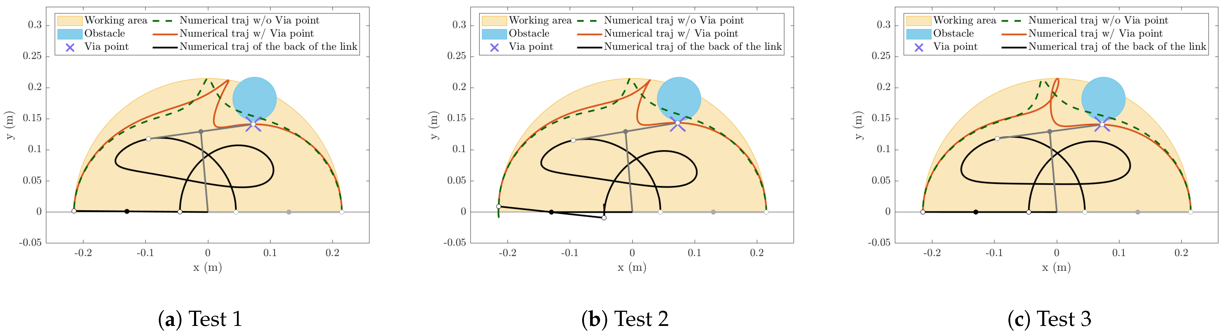
Figure 2, Figure 3 and Figure 4 show the simulated trajectory with one obstacle. The obstacle is a cylinder of radius 35 mm; the center of the base of the cylinder is placed at the point with coordinates $[75,182]$ mm in the base reference system. For completeness, in Figure 2 and Figure 4, the trajectories without via points and with the same final configuration ${\mathit{q}}_f$ and $t_f$ are shown. It is clear how the robot, without a via point, is not able to avoid the collision with the obstacle. 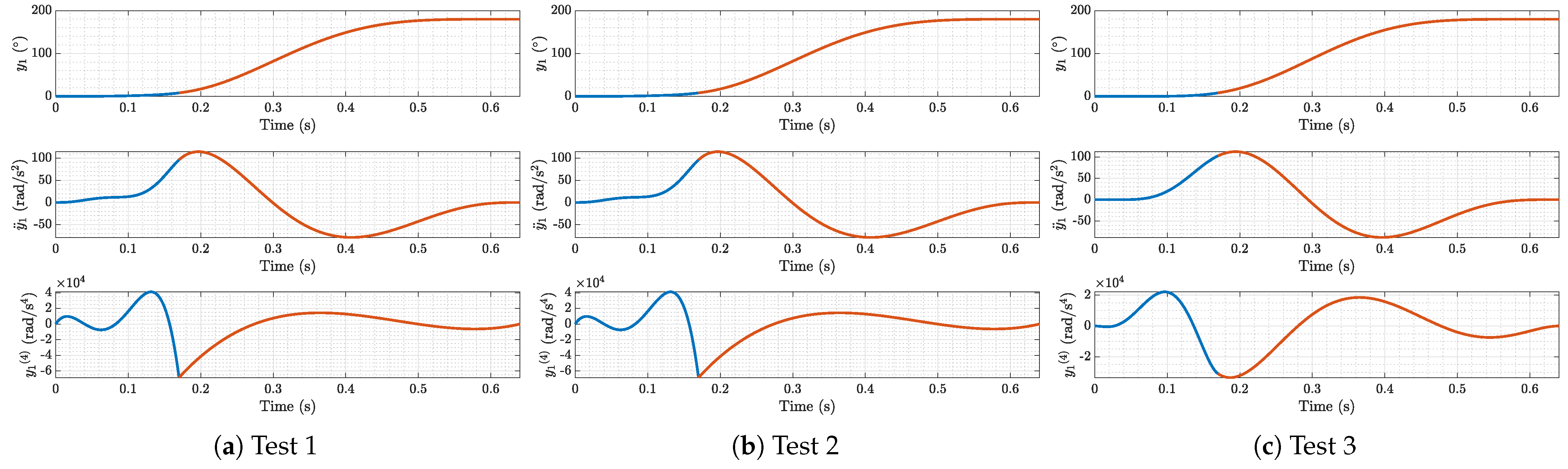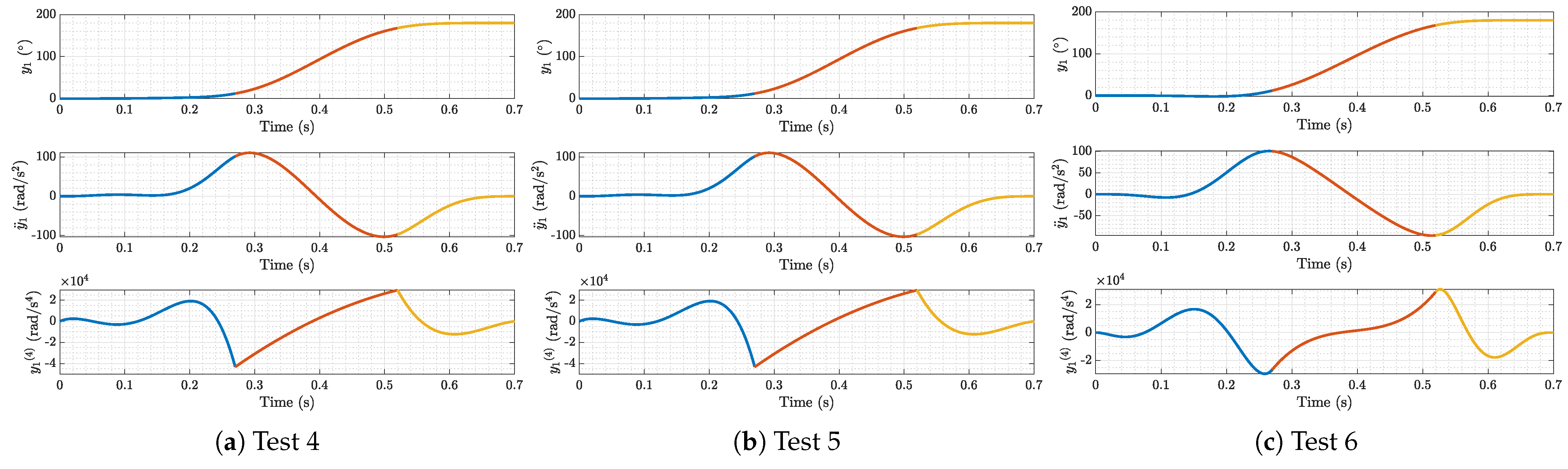The Cartesian trajectories of the end effector (Figure 2) are similar, although Test 3 (Figure 2c) shows an entangled path in the middle of the trajectory. The flat variables (Figure 3) are very similar in magnitude; this result is expected since the Cartesian trajectories are similar and the Cartesian trajectory is the result of the joint trajectories, which, in turn, are the result of the flat variables. For the flat variable derivatives, Figure 3 shows the continuity of the derivatives up to the fourth order. Moreover, the regularity of the fourth derivative of the flat variable in Test 3 confirms the continuity of the fifth derivative. The same behavior cannot be found for Tests 1 and 2.

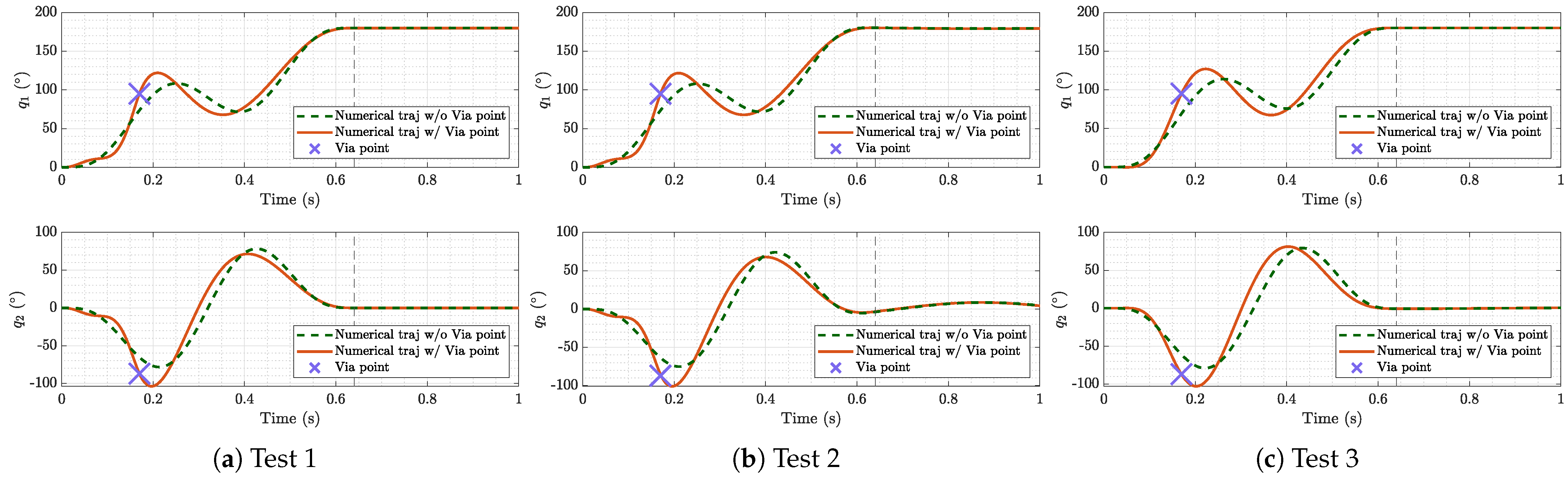
Tests 1 and 3 show no oscillations of the end effector around the final point of the trajectory (Figure 4a,c). This is an expected result since the model used for trajectory planning is the same one adopted for simulation. Conversely, the dynamic model of Test 2 is different from the one assumed in the planning phase. The result is that the robot mathematically does not exactly pass on the via point since all conditions of Section 3.2 are not met. This phenomenon is not highlighted in Figure 2b since the difference is very small; however, this difference may increase for different values of the via points ${\mathit{q}}_{via}$ and $t_{via}$. Finally, a wide natural oscillation of $q_2$ can be found after the end of the trajectory (Figure 4b).

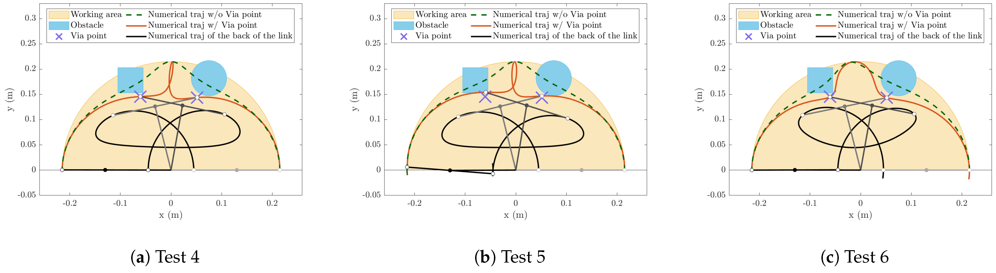
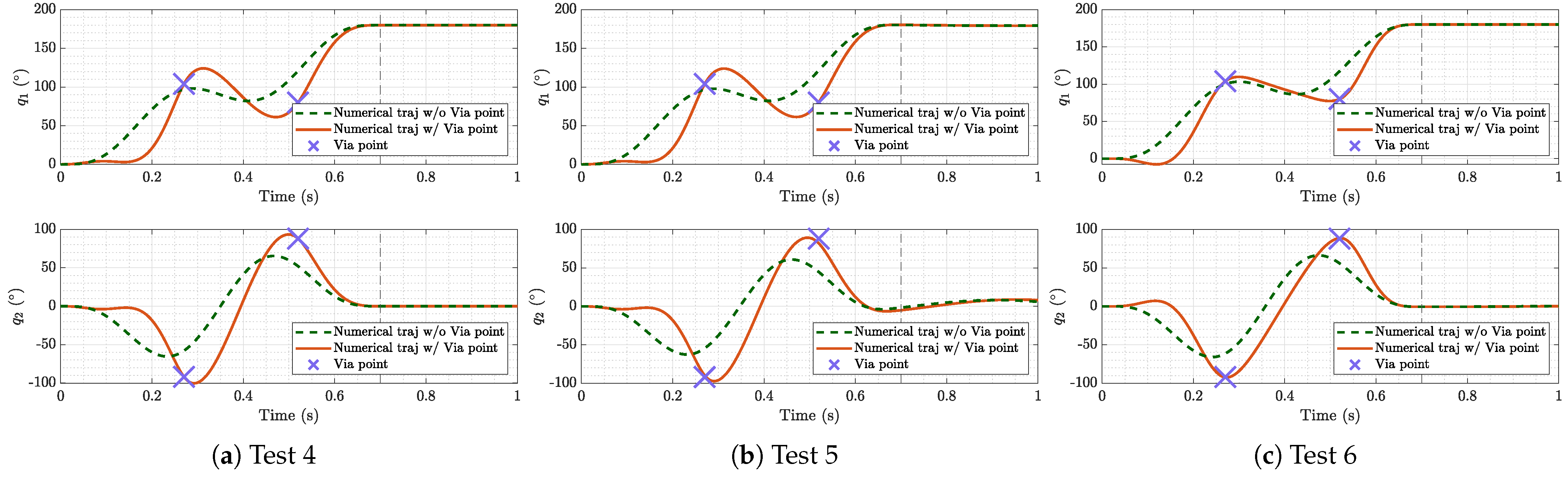
The results of the simulations with two obstacles in the workspace are reported in Figure 5, Figure 6 and Figure 7. The obstacles are the cylinder of Tests 1, 2, and 3 (in the same position) and a cube of 50 mm per side. The centroid of the cube is placed at the point with coordinates $[-80,178]$ mm in the base reference system, with the sides parallel to the base reference system axes. In this case, two via points are considered. Test 5 shows that when there is a relevant damping value, but trajectory planning is carried out neglecting damping, oscillations appear at the end of the motion, and the via points positions are not reached.

At the Cartesian trajectories (Figure 5), two results can be note. Firstly, the trajectory shapes are rather different between Tests 4, 5, and 6; this is due to the fast movements, which results in different shapes of the polynomials. In particular, the trajectory of the damped robot (Figure 5c) does not present the entanglement of Tests 4 and 5. Secondly, the trajectory of Test 5 collides with both obstacles, although the trajectory of Test 4 does not; this aspect may be crucial in very tight environments.

Finally, it is worth noting that the designer must be aware of the trajectory of the back of link 2 (black lines of Figure 2 and Figure 5) since this point may collide with the obstacle, especially for high displacements of $q_2$.

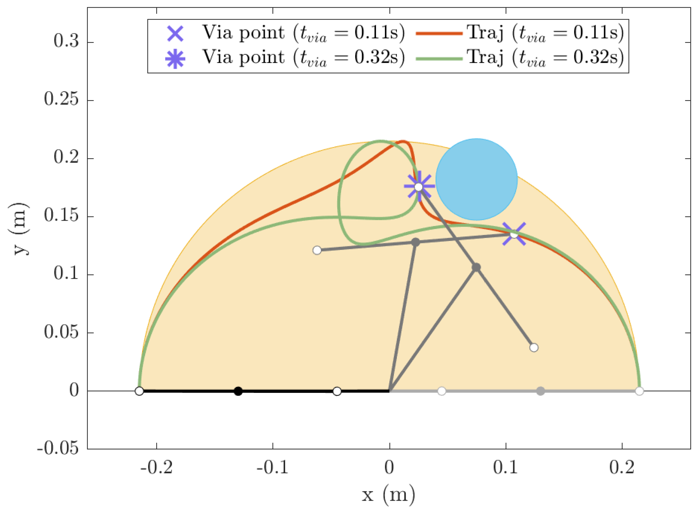
The last two tests highlight how the trajectory changes when different via points are chosen. In Figure 8, two different trajectories (orange and green lines) are shown, which are obtained with $c_n\ne 0$ and $t_f=0.64$ s (the same as Test 3) but different via points and $t_{via}$. In particular, the orange trajectory is obtained with a via point placed at ${\mathit{q}}_{via}={[80,-75]}^{\circ }$ and $t_{via}=0.11$ s; the green trajectory is obtained with a via point placed at ${\mathit{q}}_{via}={[55,70]}^{\circ }$ and $t_{via}=0.32$ s. The results show that the obstacle can be avoided with very different via points and $t_{via}$. An optimization of via point placement will be the focus of future work.

5. Experimental Validation

The proposed approach was adopted for trajectory planning of a prototype two-DOF planar underactuated robot with the same inertial properties as the one simulated in Section 4. The task of the robot was to move from one point to another, avoiding two obstacles. Although no damper was installed on the passive joint, damping phenomena due to friction were present. Friction torques are usually proportional to velocity [27]; hence, when the robot performed fast trajectories, damping could not be neglected. The experimental validation is equivalent to Test 6 of Section 4.

The first link was directly connected to the motor, which was a brushed DC motor (Portescap 35NT2R82 426SP by Mclennan Servo Supplies Ltd., Surrey, UK). The rotation of this joint was acquired by means of an incremental encoder Baumer BHK 16.05A2000-I8-5 (by Baumer Italia S.r.l., Milan, Italy) mounted on the motor. The joint was controlled using a Teensy 4.0 and employing a feed-forward control strategy with PD to compensate for uncertainties. The passive joint torsional spring stiffness ($k_2=0.0026$ Nm/rad) and damping ($c_2=2.4704\times {10}^{-5}$ Nms/rad) were identified by means of experimental modal analysis [28]. The trajectory of link 2 was recorded using a high frame-rate camera for industrial use (Dalsa Genie Nano GM30-M2050 by Teledyne DALSA, Waterloo, ON, Canada) that detects the white markers fixed to the second link. For this camera, at the maximum resolution ($2064\times 1544$ pixels), the maximum frame rate is 187 fps. However, the frame rate was increased to 280 fps by setting a region of interest (ROI) of dimensions $1600\times 800$ pixels.

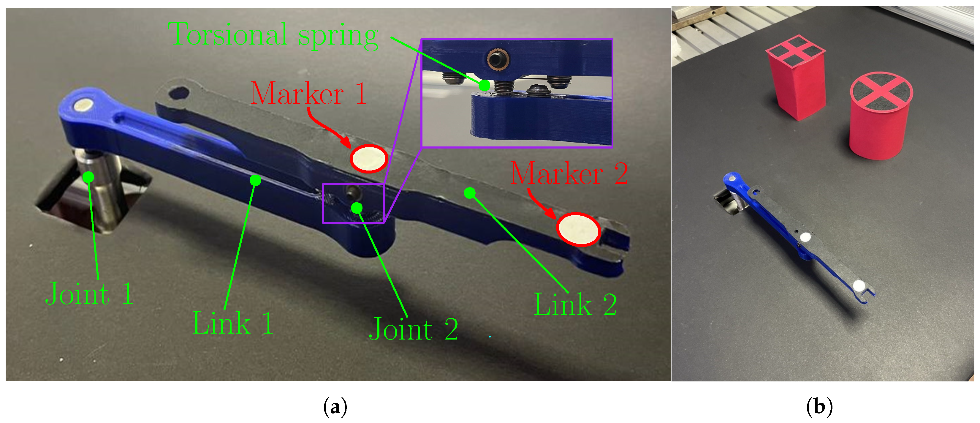
The test setup is shown in Figure 9a. To replicate the simulation, a paper cylinder and a paper cube were placed in the work area in the same position as in the simulation. The two obstacles are shown in Figure 9b. The movement was performed with the via points of Test 6 but with a different set of $t_{via}$ ($t_{via}=0.175$ s for the first via point, and $t_{via}=0.4185$ s for the second via point).

Before the recording, the camera was calibrated on the plane containing the markers to remove any distortions and to ensure a correct mm/pixel ratio. The camera feed was post-processed after the robot movement, and the marker positions were measured. The coordinates of marker 2 (Figure 9a) were compared to the end effector trajectory of the numerical simulation (i.e., the point placed at a distance $a_2$ with respect to joint 2). At the same time, since no position sensors were located on joint 2, the joint trajectory $q_2\left(t\right)$ was obtained by measuring the absolute angle of the line connecting marker 1 and 2 and by subtracting the joint 1 trajectory $q_1\left(t\right)$.

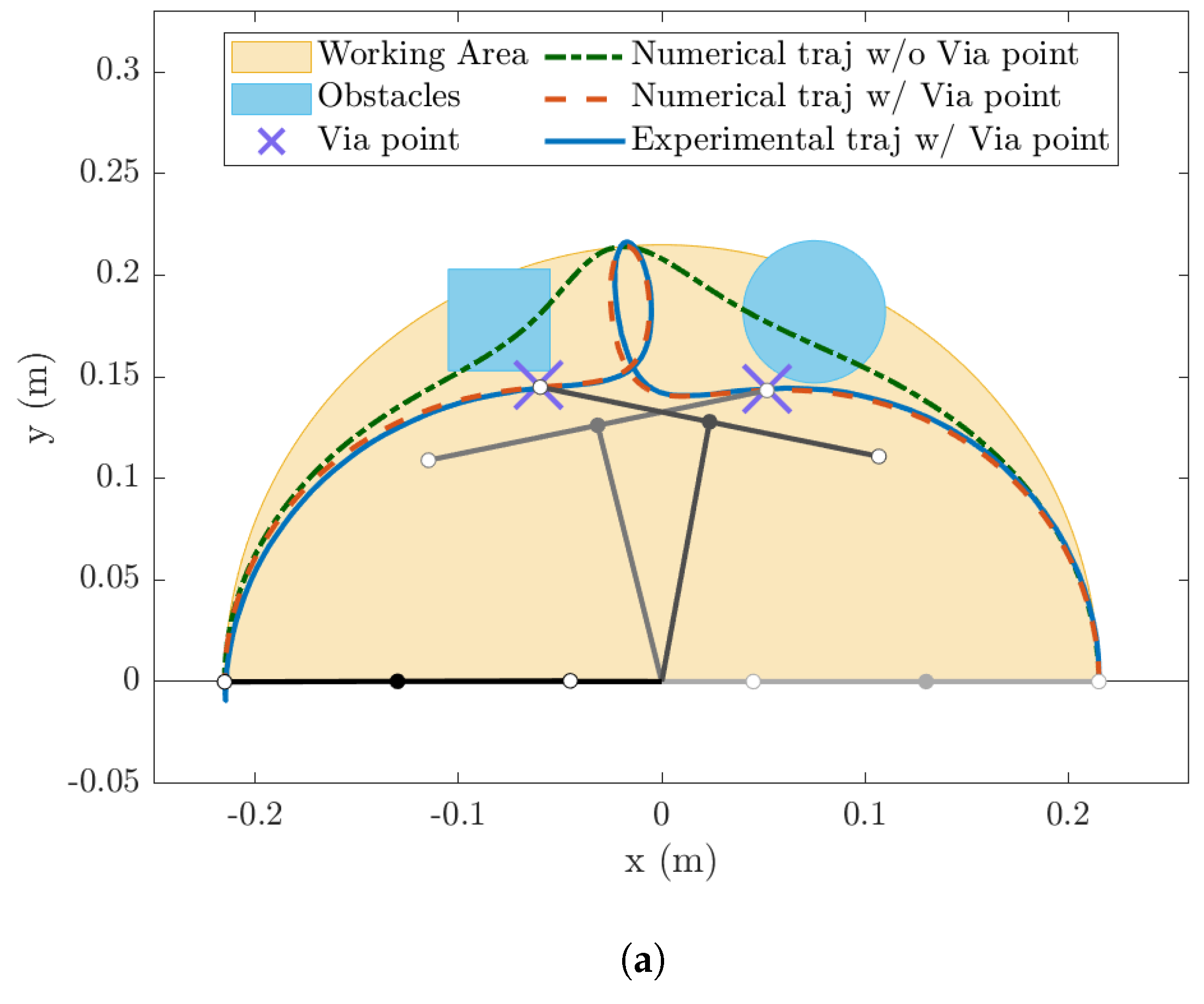
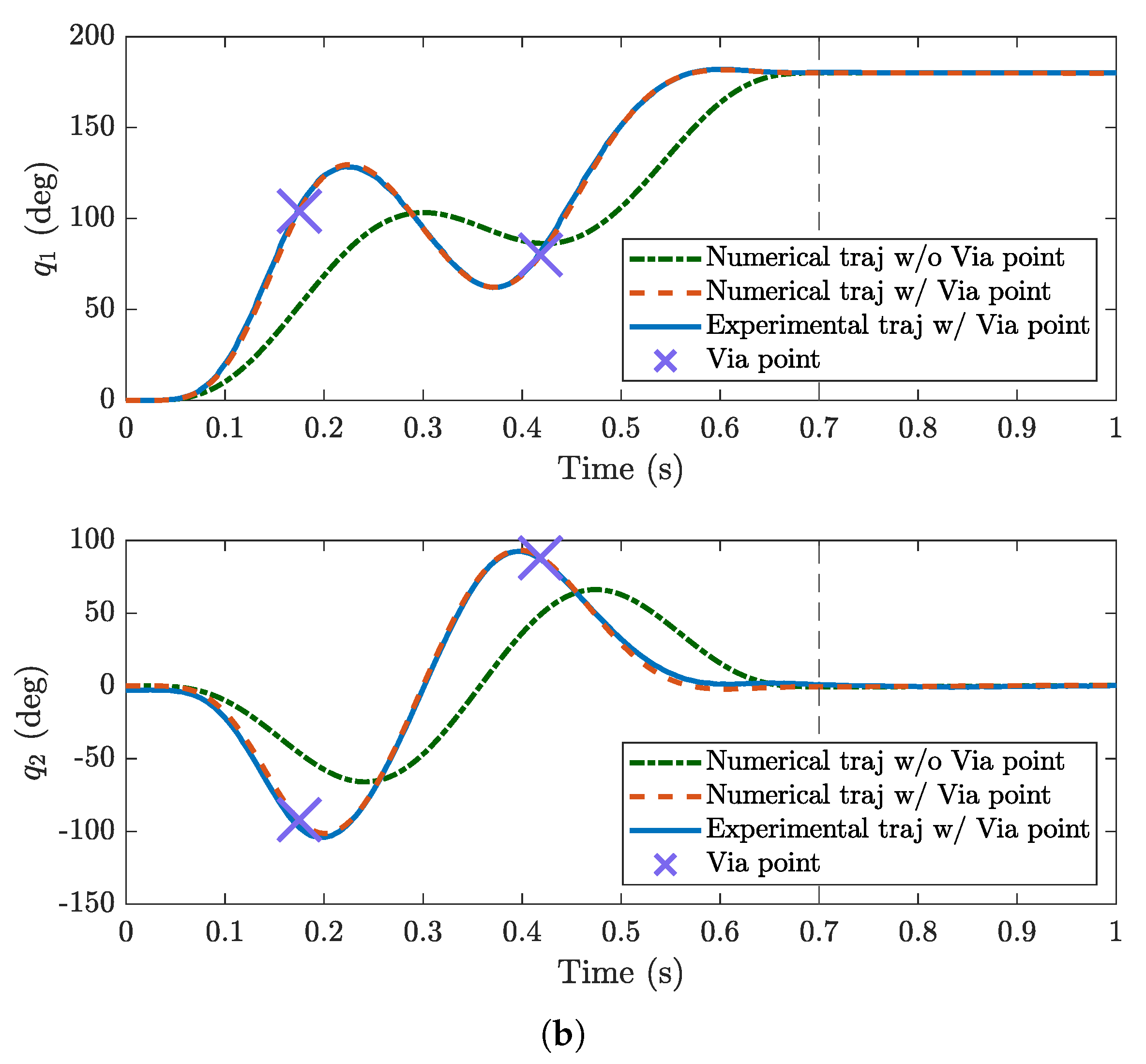
Both Cartesian and joint trajectories (Figure 10a and Figure 10b, respectively) showed very good agreement between experimental and numerical results. The overshoot that can be seen at the end of the Cartesian trajectory is present both in the numerical and experimental trajectories and is due to robot dynamics. The robot was able to reach the via points according to the planning, and no noticeable oscillations of the passive joint were present at the end of the movement. It is worth noting that the movement was very fast ($t_f=0.7$ s); thus, the inertial forces play a relevant role in the system dynamics. The fact that the robot is differentially flat ensures that the centrifugal and Coriolis forces of the last links are zero; thus, the dynamic model becomes very accurate.

The result was obtained without having any feedback on the position of the last joint; in fact, both the Cartesian and joint trajectories were post-processed from the video captured by the camera and were not used in the control system. Conversely, the robot was driven by calculating the trajectory of the first joint after the planning of the flat variable and the employment of the dynamic model.

6. Conclusions

The main contribution of this paper is the development and validation of a method for motion planning in the space of flat variables considering the presence of via points. It is an extension of the approach adopted for point-to-point motion. A general formulation with $n_{via}$ via points and the flat variables interpolated by high-order polynomial functions has been presented. Since the number of flat variables is lower than the number of DOFs, the indetermination of the configuration of the robot at the via point is solved, adding another condition that comes from the equations of motion.

A series of numerical simulations and an experimental test on a prototype were carried out to assess the validity of the proposed method. The results show that the introduction of one or more via points strongly increases the possibility of avoiding obstacles in the workspace. The numerical results show that the trajectories of the robot in the Cartesian space depend on the position of the via points, the total duration of the motion, and the duration of the various motion sections between the via points.

Since, in actual industrial applications, these parameters can be varied within assigned ranges, future research will deal with the optimization of these parameters. The goal of the optimization can be the minimization of the distance from the obstacles or the minimization of the torques demanded by the actuated joints for an assigned distance of the robot path from the obstacles. Further developments will deal with the interpolation of the flat variables by means of different families of functions as well.