Designing Digital Twins of Robots Using Simscape Multibody

Abstract

Digital twins of industrial and collaborative robots are widely used to evaluate and predict the behavior of manipulators under different control strategies. However, these digital twins often employ simplified mathematical models that do not fully describe their dynamics. In this paper, we present the design of a high-fidelity digital twin of a six degrees-of-freedom articulated robot using Simscape Multibody, a Matlab toolbox that allows the design of robotic manipulators in a rather intuitive and user-friendly manner. This robot digital twin includes joint friction, transmission gears, and electric actuators dynamics. After assessing the dynamic accuracy of the Simscape model, we used it to test a computed torque control scheme, proving that this model can be reliably used in simulations with different aims, such as validating control schemes, evaluating collaborative functions or minimizing power consumption.

1. Introduction

The use of simulators in robotics research is widespread, as it supports the development of new devices and the design, validation, and comparison of different control strategies. Robot simulations can be performed for a variety of purposes, ranging from path planning to generating data for learning-based approaches. Many different robotic simulators are available, and they are usually preferred over each other depending on the scope of the simulation and the background of the person carrying it out, as robotics is a multidisciplinary field.

The first aim of robotic simulations is typically to analyze robots from a kinematic point of view, which includes workspace investigation, path planning verification and optimization, and collision avoidance. This only requires a kinematic model of the robot and a 3D visual representation of the manipulator in its working environment. In addition to kinematic analysis, dynamic analysis (i.e., predicting the torques necessary to perform a desired motion) is of paramount importance for robot control design, actuator dimensioning, and collaborative functions evaluation. For this purpose, dynamic models of increasing complexity have been developed, taking into account actuators dynamics, the flexibility introduced by belts and harmonic drives, and the possible interaction between the robot and the environment. In the later stage of the design process, real-time robotic simulations are useful to evaluate the computational efficiency of control strategies.

Most robot manufacturers developed their own proprietary simulators, such as RoboGuide [1] for Fanuc robots, Automation Control Environment (ACE) [2,3] for Omron robots, or Robotstudio [4,5] for ABB robots. These simulators are very useful for offline programming, path planning, and collision avoidance, as they allow 3D visual representation of the robot in virtual environments. Even though these proprietary software sometimes provide information on required torques and power consumption, the dynamic model used to derive such values is not known and the actual control algorithms implemented by the robot manufacturers are unavailable. For this reason, for custom-made robots and more advanced simulations, generic simulation software needs to be used. A comprehensive review of the available simulators specifically developed for robots has recently been presented in [6], the most used of them being Gazebo, Webots and Coppeliasim. Less often, robots are modeled and simulated using a multibody approach. The multibody model of a manipulator and, more generally, of a mechanical system, is composed of rigid and deformable bodies, interconnected by means of kinematic pairs. Among the available multibody dynamics software, Simscape Multibody [7] (formerly SimMechanics), is a powerful Matlab/Simulink toolbox that can be used to simulate the behavior of complex mechanical and robotic systems. In particular, it also allows the inclusion of external forces acting on the robot, which is particularly important when simulating human-robot interaction. Simscape Multibody is fully integrated within the Matlab framework and thus easy to use in conjunction with other toolboxes, such as Simscape Mechanical to add joint rotational friction, Simscape Driveline to add reduction gears, and Simscape Electrical to include actuator dynamics. In addition, it is also integrated with the Robotic System Toolbox [8], a well-established Matlab toolbox for robot simulation. Simulink, being the most widely used simulation platform in control theory verification, also allows users to build block diagrams of high- and low-level robot control loops. For these reasons, Simscape Multibody is a perfect candidate to build high-fidelity digital twins of robots. In fact, Simscape Multibody has already been successfully used in the field of robotics to build models of articulated [9,10,11,12,13,14,15,16,17], parallel [18,19], mobile [20,21] and legged robots [22,23]. It has also been used to test a robot dynamic parameter identification method in [24], to test robot control strategies in [25,26,27,28], to model and simulate a multi-fingered robot arm grasping [29] and to design a 5 degrees of freedom manipulator for additive manufacturing in [30]. However, previous studies using Simscape Multibody have mostly focused on the kinematic modeling of robots, neglecting its dynamic modeling and the inclusion of non-idealities, friction, reduction gears, and motor dynamics. Only in [9,11] friction was included and only in [11,30] the motor dynamics was taken into account. Nevertheless, while robot manipulators are typically equipped with Permanent Magnet AC Synchronous Motors (PMSMs), in [11] PMSMs motors were described through their simplified equivalent DC monophase models while in [30] bruslhess DC servomotors were modeled. This approach is sufficient if the aim of the simulation is to take into account the motor dynamics and their saturation limits, but if the aim of the simulation is to develop a custom robot controller and servo drives, the robot model should have a level of detail to the motor inverters. Furthermore, none of the previous studies exploited the algorithms of the Robotic System Toolbox in conjunction with Simscape Multibody to assess their capabilities and limitations in complex robotic simulations.

In this paper, we present how high-fidelity digital twins of robots can be designed in a rather intuitive and user-friendly manner using Simscape Multibody. The major novelity of the present work regards the integration of the robot model created in Simscape Multibody environment with a comprehensive model of friction, reduction gears, and motor dynamics. Taking into account complete models of non-idealities allows more accurate prediction of the robot’s behavior under different control strategies, while taking into account PMSMs dynamics allows to simulate the control scheme with a level of detail to the switch inputs of the motors inverters, which is particularly important in robots with custom servo drives. In addition, we compared the algorithms of the Robotic System Toolbox (i.e., algorithms for direct and inverse kinematics, forward and inverse dynamic) with mathematical models derived in a classical way [31,32] to assess their accuracy and computational efficiency in real-time robot simulations. We believe that the approach and results presented in this work will be greatly useful to other researchers whose aim is to develop custom robots with dedicated kinematics, controller and servo drives.

The remainder of this paper is organized as follows: in Section 2 the model of a manipulator is built within the Simscape environment, the algorithms for direct and inverse kinematics are tested, and their computational efficiency is compared. In Section 3 dynamic simulations are carried out to verify the correctness of the manipulator’s model under ideal conditions, comparing the output of the Simscape model with mathematical models derived using both the Euler-Lagrange and Newton-Euler approaches. In Section 4 friction, reduction gears, and motor dynamics are included in the model, and in Section 5 a computed torque control is implemented. Finally, in Section 6 our conclusions are drawn.

2. Kinematic Modeling

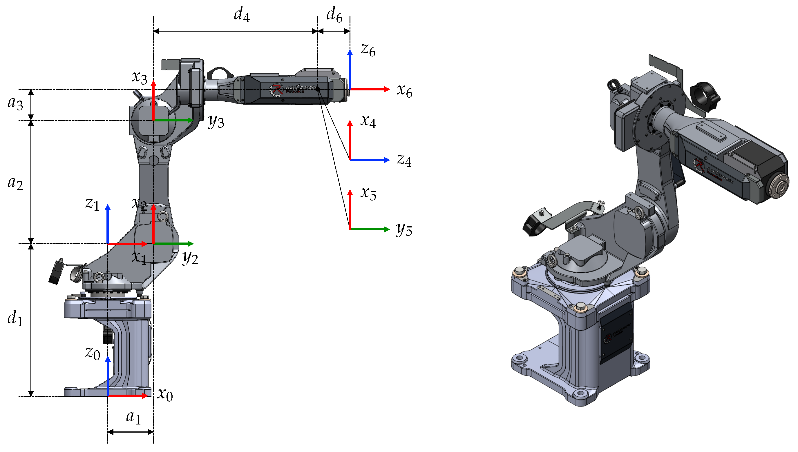
2.1. Kinematic Description of the Manipulator

In this work, we created a digital twin of a six degree-of-freedom (DOF) articulated robot with a spherical wrist, which is the most common architecture for industrial robots. As an example, we modeled the AT_00011 manipulator from Autonox Robotics GmbH [33]. While most robot manufacturers provide their own proprietary software for offline programming and 3D simulation, as stated in Section 1, Autonox is a company that produces independent robot mechanics that can be controlled through different controllers and a simulation environment for Autonox robots is not available. For this reason, we believe that modeling this robot is particularly relevant to show the effectiveness of the proposed approach.

From a multibody point of view, a 6 DOF anthropomorphic robot is composed of a base and six bodies (typically referred to as links), each interconnected through a revolute joint. Kinematic modeling in robotics is usually carried out following the Denavit Hartenberg (DH) convention [34], which affixes frames to the various parts of the manipulator and then describes the relationships between these frames. The 6 DOF anthropomorphic robot with attached DH frames according to the convention described in [31] is reported in Figure 1, while the DH parameters are presented in

Table 1. DH parametersof a 6 DOF anthropomorphic robot.

i	${}^{\mathit{i}-1}\mathit{T}_{\mathit{i}}$	${\mathit{\alpha }}_{\mathit{i}-1}$	${\mathit{a}}_{\mathit{i}-1}$	${\mathit{\theta }}_{\mathit{i}}$	${\mathit{d}}_{\mathit{i}}$
		${(}^{\circ })$	(mm)	${(}^{\circ })$	(mm)
1	${}^0\mathit{T}_1$	0	0	${\theta }_1$	500
2	${}^1\mathit{T}_2$	$-90$	150	${\theta }_2$	0
3	${}^2\mathit{T}_3$	0	400	${\theta }_3$	0
4	${}^3\mathit{T}_4$	$-90$	100	${\theta }_4$	540
5	${}^4\mathit{T}_5$	90	0	${\theta }_5$	0
6	${}^5\mathit{T}_6$	$-90$	0	${\theta }_6$	100

.

The homogeneous transformation matrix from frame $i-1$ to frame i can be easily calculated from the DH table as

$${}^{i-1}\mathit{T}_i={\mathit{R}}_x\left({\alpha }_{i-1}\right){\mathit{D}}_x\left(a_{i-1}\right){\mathit{R}}_z\left({\theta }_i\right){\mathit{D}}_z\left(d_i\right),$$

(1)

where $\mathit{R}$ represent a rotation matrix and $\mathit{D}$ represent a translation matrix and the subscript indicates the axis of rotation/translation. As a result, the direct kinematics of the manipulator (i.e., the homogeneous transformation matrix from the base frame to the end-effector frame) is calculated as

$${}^0\mathit{T}_6={}^0\mathit{T}_1{}^1\mathit{T}_2{}^2\mathit{T}_3{}^3\mathit{T}_4{}^4\mathit{T}_5{}^5\mathit{T}_6.$$

(2)

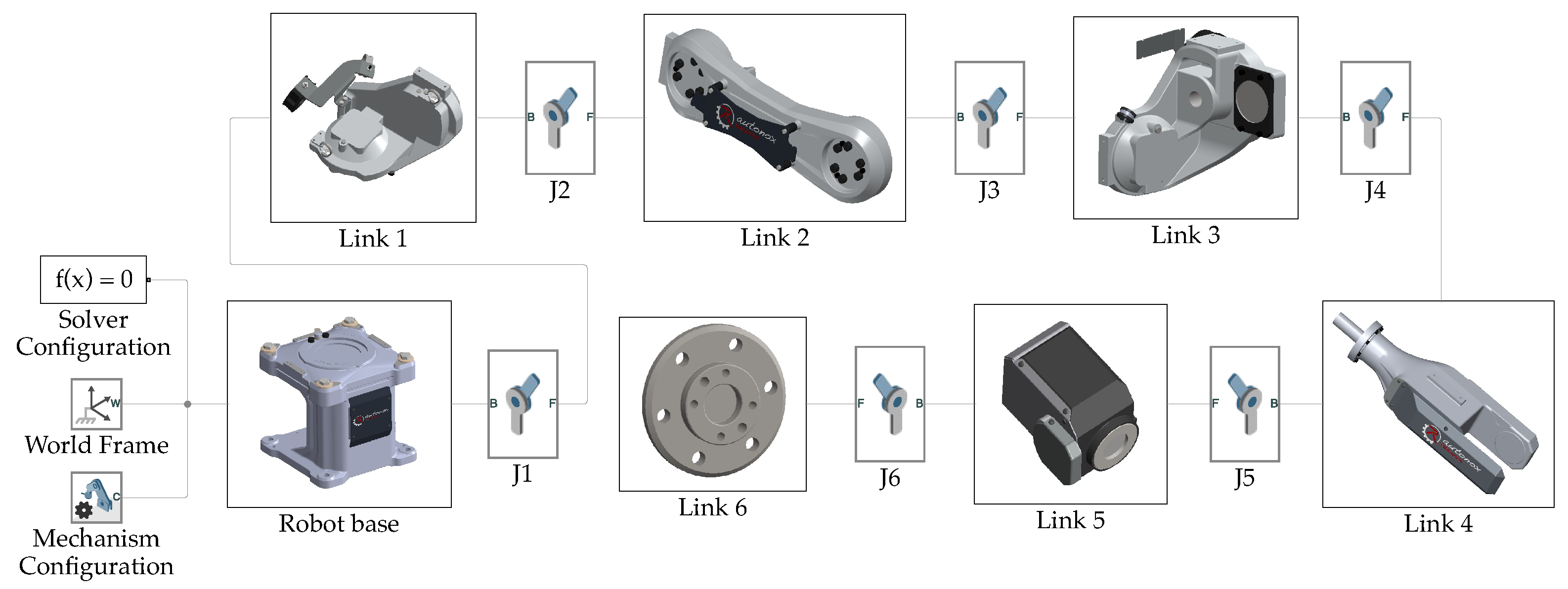
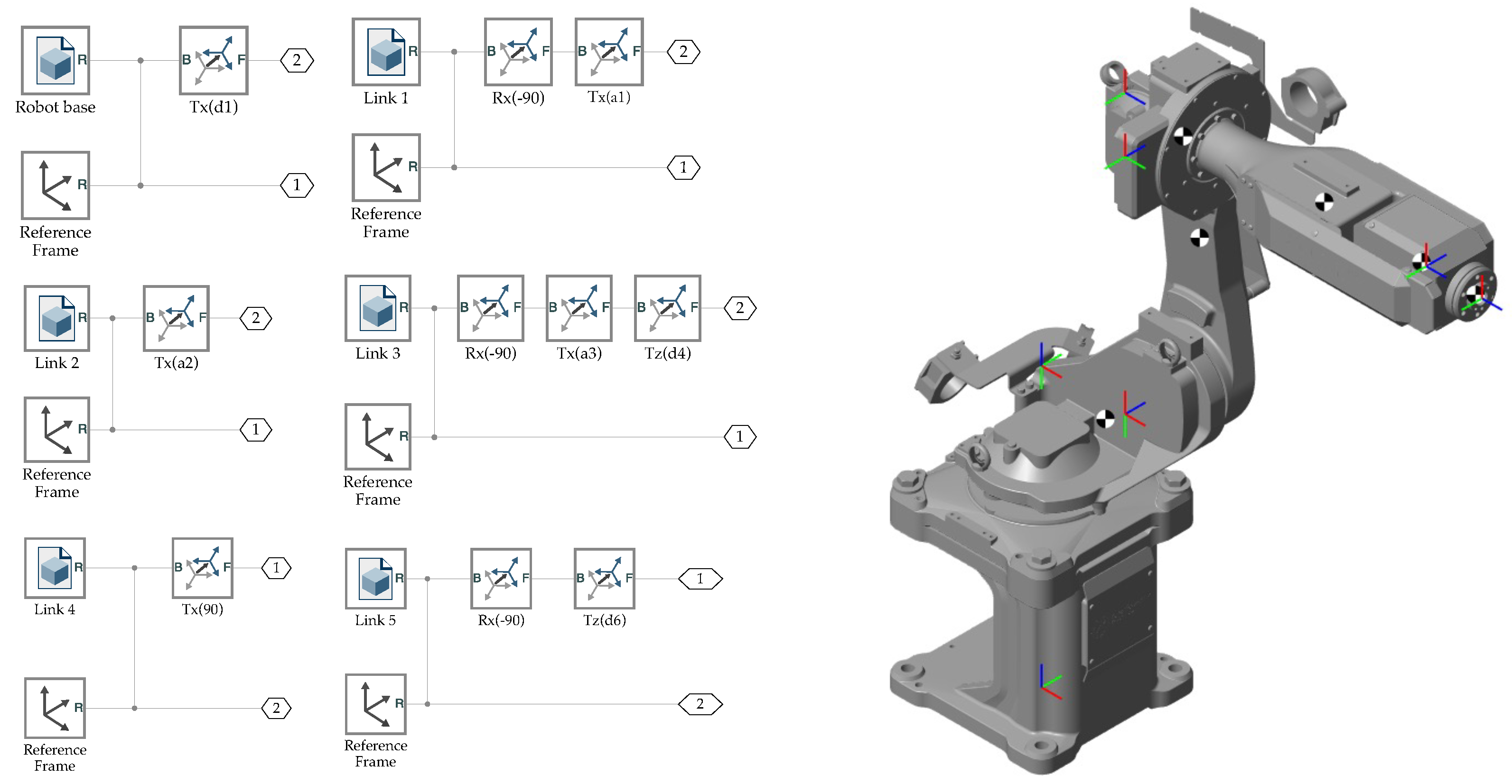
2.2. Creation of the Robot Kinematic Model in Simscape Multibody

In the Simscape Multibody simulation environment, a multibody system is modeled using blocks representing bodies, joints, constraints, and forces. In particular, each body is characterized by a geometry typically derived from a CAD file, a mass, a local reference frame, the coordinates of the center of mass (CoM) with respect to the local reference frame, and the inertia tensor relative to a frame with origin at the center of mass and axes parallel to the local reference frame. The position of the local reference frame depends on the original CAD file, while the mass, center or mass and inertia tensor can be parametrized using Matlab variables or determined directly by Simscape based on the geometry and on the density of a body’s material. Bodies are subsequently interconnected by means of joints and proper constraints specified in terms of relationships between local reference frames. The Simscape Multibody solver then automatically builds a system of differential agebraic equations (DAE) of motion [35] where the bodies are modeled as rigid elements and the kinematic pairs as algebraic constraints.

The first step in designing a robot digital twin using Simscape Multibody is to prepare its 3D CAD model. The CAD assembly of manipulators can usually be found on the manufacturer’s website. Simscape Multibody allows users to create the multibody model by directly importing a CAD assembly model file from external 3D CAD (such as SolidWorks or Autodesk Inventor). This is made possible by Simscape Multibody Link, an add-on for the CAD software that generates an XML file of the assembly and an STL file of each body. The XML file can then be imported into MATLAB with the command smimport, which automatically generates the blocks representing bodies, joints, and constraints between bodies. However, depending on how each link has been designed in the CAD environment (i.e., where its origin is located) and how the assembly constraints have been defined, this import can generate unnecessary constraints and transformations between bodies and joints, especially for custom-made robots with a high number of DOFs. As the relationships between bodies are specified in terms of translation and rotations from one local reference to another, we found that the most effective way to generate a Simscape Multibody model of a robot is to define in the CAD software, for each link, a reference frame located at the corresponding DH frame and then import each body separately. Following this approach, the local reference frame of each link corresponds to its DH frame, and the translations and rotations from one local reference to another, which have to be manually defined, correspond to the ones specified in the DH table.

The complete Simscape Multibody model of the 6 DOF anthropomorphic robot obtained through the described procedure is reported in Figure 2: each link of the robot is represented by a subsystem, which contains the part CAD file and the necessary transformations to connect it to the next link. The subsystem of each link is shown on the left in Figure 3, where the transformations between each body, which correspond to Equation (1), can be seen explicitly. Once the simulation is started, the 3D visualization of the robots with attached frames and center of masses appears in the Mechanics Explorer utility and is reported on the left in Figure 3.

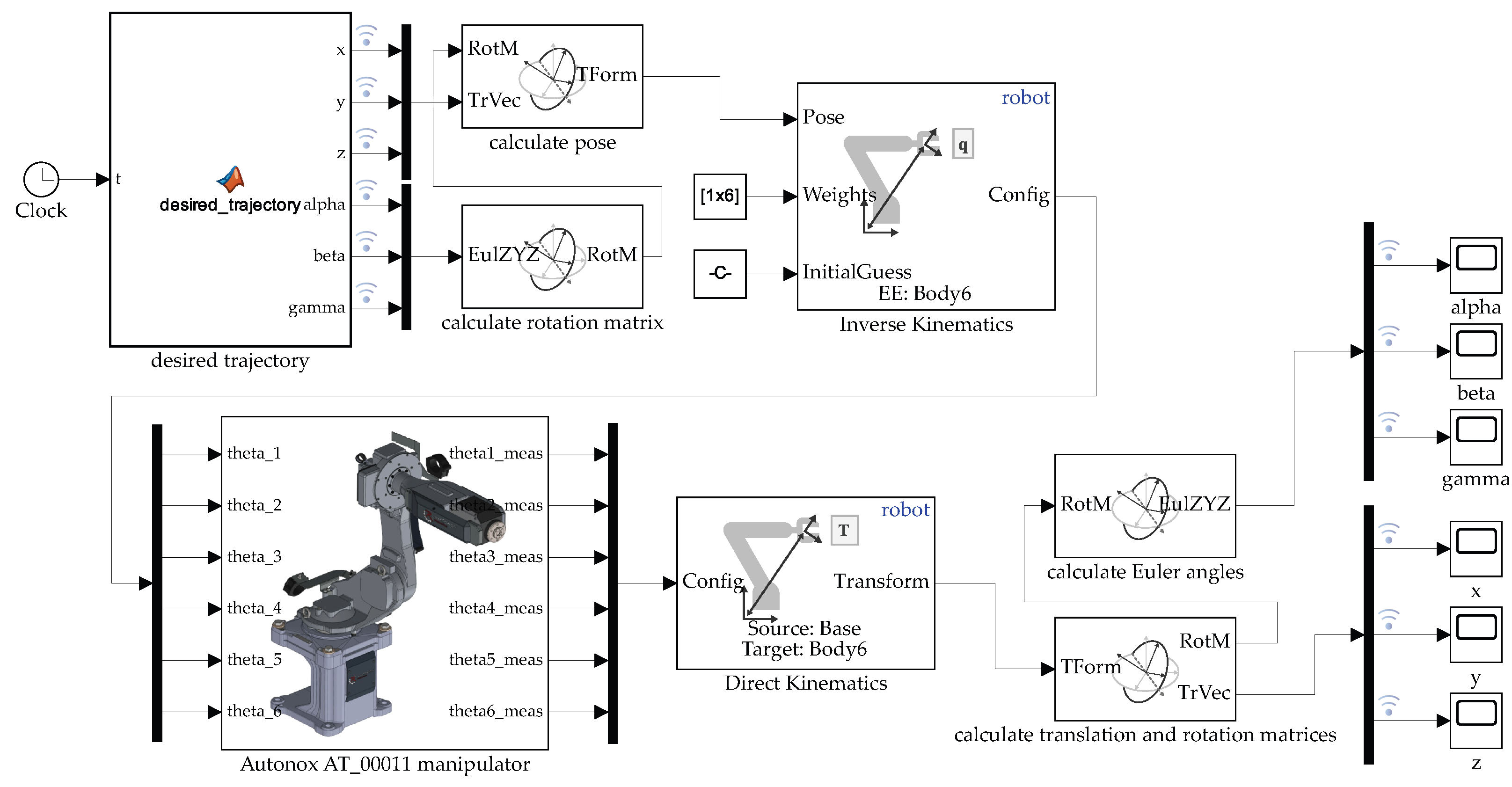
2.3. Interface with the Robotic System Toolbox

A widely used MATLAB toolbox to design, test and simulate robotic applications is the Robotic System Toolbox, originally developed by Dr. Peter Corke [36]. This toolbox, in the Simulink environment, provides a number of blocks to perform coordinate transformations, direct and inverse kinematics and dynamics, to calculate robots Jacobians, and to generate trajectories. These blocks are very useful and easy to use, without requiring advanced knowledge in the field of robotics.

Each block of the Robotic System Toolbox requires a rigidBodyTree object as input, which is the class used to build robot models. To use these blocks for the robot modeled using Simscape Multibody and depicted in Figure 2, we used the importrobot command, which returns a rigidBodyTree object.

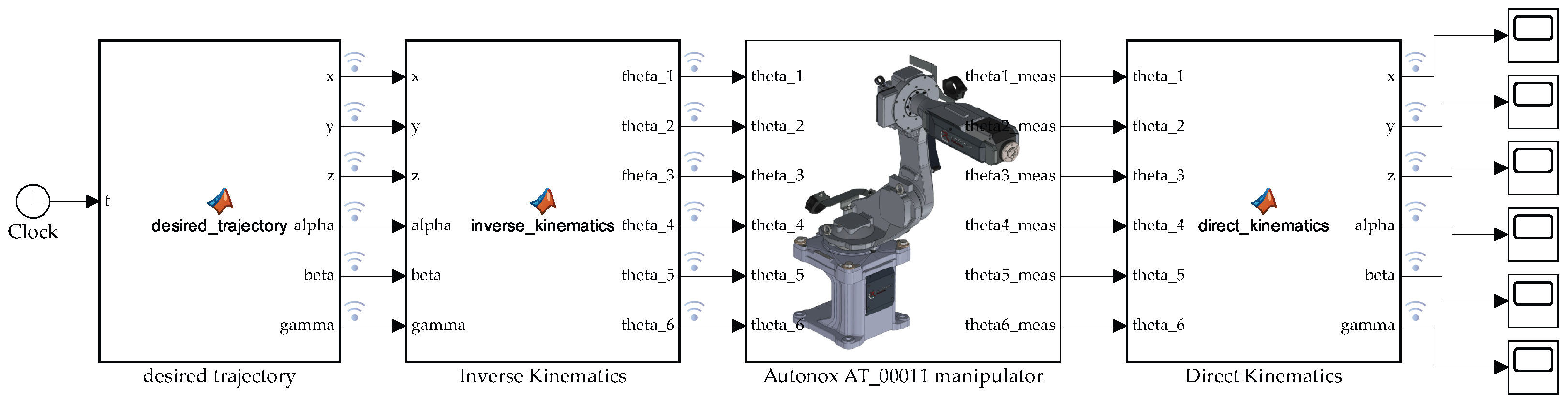
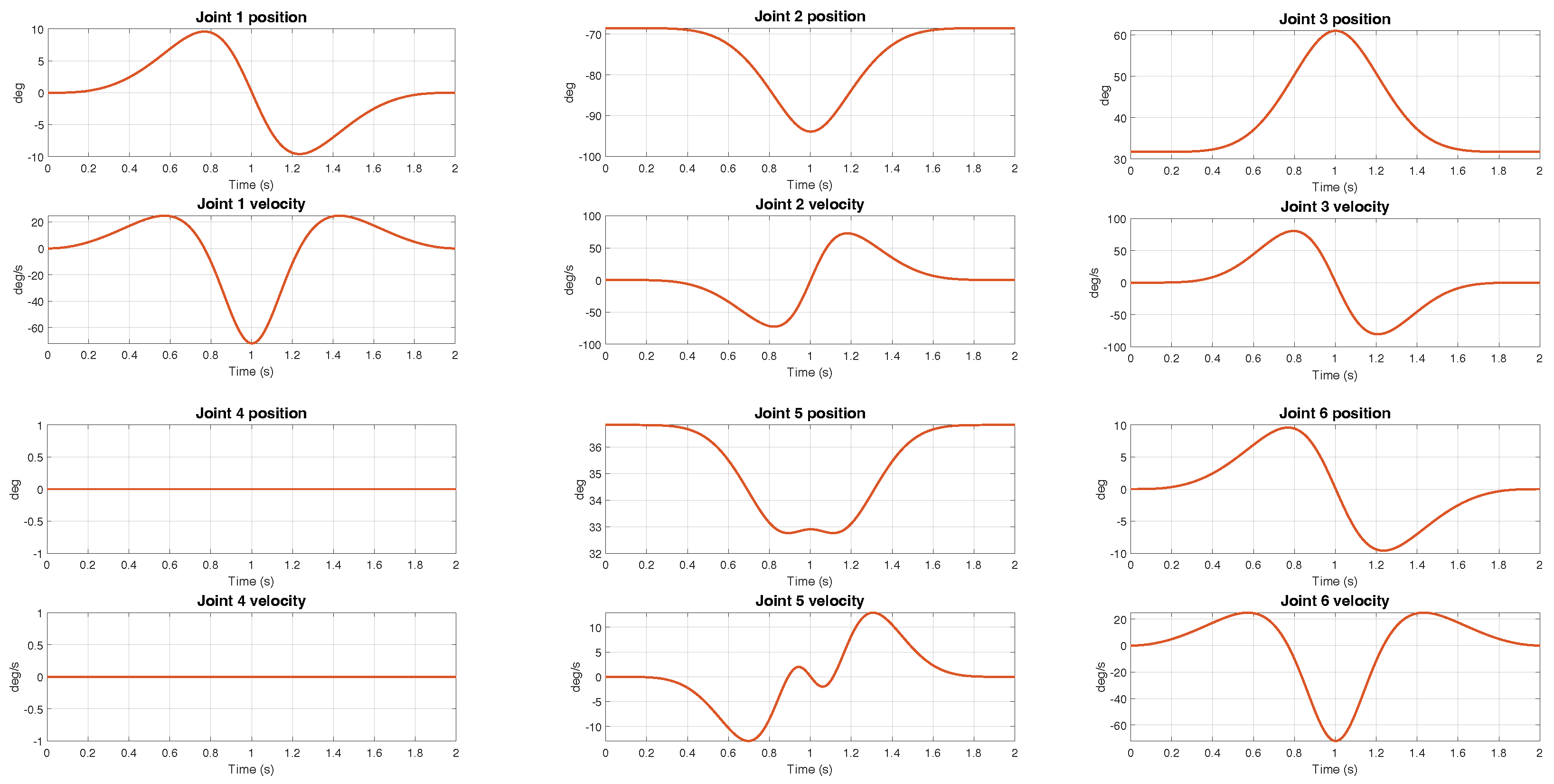
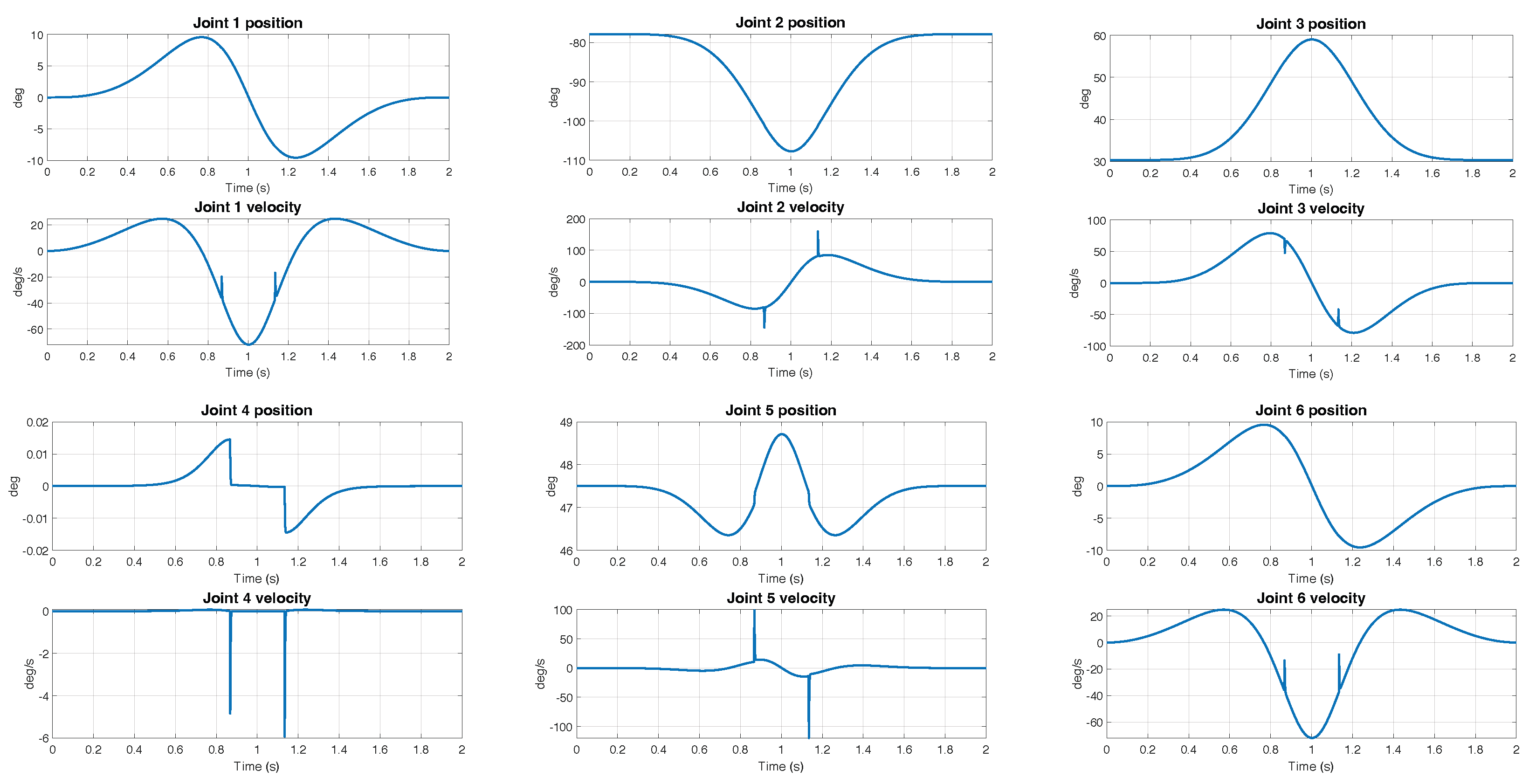
2.4. Kinematic Control of the Manipulator in the Cartesian Space

In the Simscape model depicted in Figure 2 the joints are not actuated (there is no position or torque input): under these conditions, when the simulation starts, the robot falls under the effects of gravity (whose value is specified in the Mechanism Configuration block). For each joint, the torque and position can be alternatively provided by input or automatically computed, meaning that each joint can be torque controlled or position controlled. For kinematic simulations, as the ones described in this section, the position is provided by input, while the torque is automatically computed. For dynamic simulations, such as those described in Section 3, the torque is provided by input, while the position is automatically computed.

As an example, here we show how the kinematic control of the manipulator in the Cartesian space can be performed in the Simscape Multibody environment both exploiting user-defined Matlab functions and Robotic System Toolbox functions, and we compare their accuracy and computational efficiency. Without loss of generality, we considered a circle in the XY plane as the desired trajectory. More in detail, the angle $\theta \left(t\right)$ is defined as a sinusoidal trajectory:

$$\theta \left(t\right)=2\pi \left[\frac{t-t_0}{T}-\frac{1}{2\pi }sin\left(2\pi \frac{t-t_0}{T}\right)\right],$$

(3)

where the initial time is $t_0=0 \mathrm{s}$ and the total time of motion is $T=2 \mathrm{s}$. The trajectory is then specified in the Cartesian space in terms of the desired $(z,y,z)$ coordinates and $(\alpha ,\beta ,\gamma )$ ZYZ Euler angles:

$$\left\{\begin{array}{c}{x}_d\left(t\right)=x_{d_0}+rcos\left(\theta \left(t\right)\right)\hfill \\ y_d\left(t\right)=y_{d_0}+rsin\left(\theta \left(t\right)\right)\hfill \\ z_d\left(t\right)=z_{d_0}\hfill \end{array}\right.\left\{\begin{array}{c}{\alpha }_d\left(t\right)={\alpha }_{d_0}\hfill \\ {\beta }_d\left(t\right)={\beta }_{d_0}\hfill \\ {\gamma }_d\left(t\right)={\gamma }_{d_0}\hfill \end{array}\right.,$$

(4)

where $x_{d_0}=600 \mathrm{m}\mathrm{m}$, $y_{d_0}=0 \mathrm{m}\mathrm{m}$, $z_{d_0}=500 \mathrm{m}\mathrm{m}$, $r=100 \mathrm{m}\mathrm{m}$, ${\alpha }_{d_0}=0^{\circ }$, ${\beta }_{d_0}={180}^{\circ }$ and ${\gamma }_{d_0}={180}^{\circ }$.

To perform a trajectory in the Cartesian space, inverse kinematics needs to be computed. The inverse kinematics of a 6 DOF articulated robot with a spherical wrist is a well-known issue in robotics, and its closed form solution can be easily found in [31,32] and can be implemented in Simulink as a user-defined function. Once the joints values necessary to perform the trajectory have been calculated, they are provided as inputs to the revolute joints of the Simscape Multibody robot model. The joint positions are then measured and used to compute the direct kinematics, and therefore the actual position and orientation of the end-effector. Figure 4 shows how the kinematic control of the 6 DOF anthropomorphic robot manipulator can be obtained using user-defined Matlab functions. The same kinematic control of the robot can also be obtained by exploiting the Robotic System Toolbox blocks, as shown in Figure 5. In particular, the Robotic System Toolbox provides a block that calculates the inverse kinematics through an iterative gradient-based optimization method. This block requires as inputs the rigidBodyTree object (derived as in Section 2.3), the desired pose, the weights, and the initial guess. A number of solver parameters can be modified by the user, such as the exit conditions, which determine both the accuracy of the solution and the time needed to carry out the simulation. The desired pose is specified in terms of a homogeneous matrix, which is obtained by a rotation matrix and a rotation matrix through the Coordinate Transformation Conversion block. The rotation matrix is in turn obtained from the ZYZ Euler angles through another Coordinate Transformation Conversion block. Similarly, the Direct Kinematics block calculates the direct kinematics from the measured joint values: the output of this block is a homogeneous matrix, which is subsequently transformed into $(x,y,z)$ and $(\alpha ,\beta ,\gamma )$ coordinates through Coordinate Transformation Conversion blocks.

In fact, the Robotic System Toolbox blocks allow users to perform a trajectory in the Cartesian space even without explicit knowledge of the direct and inverse kinematic problems, but their use poses some limitations i.e., discontinuities in joint velocities and a longer simulation time. Figure 6 shows the measured joint positions and velocities obtained from the simulation with user-defined Matlab functions, while Figure 7 shows the ones obtained from the control scheme that uses Robotic System Toolbox blocks. The joint velocities measured during the simulation that uses Robotic System Toolbox blocks present two discontinuities around $t_1=0.85 \mathrm{s}$ and $t_2=1.15 \mathrm{s}$: these spikes depend on the inverse kinematic solver parameters and can be eliminated by decreasing the value of exit conditions. On the other hand, the average elapsed time of the simulations using two different algorithms for the inverse kinematics is reported in

Table 2. Elapsed time of the kinematic control simulation using the two different algorithms.

	User-Defined Closed Form	Robotics System Toolbox
Average elapsed time	$1.74 \mathrm{s}$	$30.19 \mathrm{s}$

: regardless of the solver parameters, carrying out the simulation that uses Robotic System Toolbox blocks always takes much longer than the one that uses user-defined Matlab functions, and this is due to the iterative nature of the solver for the Inverse Kinematics, as the stability of the numerical solution and its convergence rate cannot be guaranteed. In addition, when more than one solution to the inverse kinematics is possible, the user-defined function allows the user to choose the robot configuration, while the Inverse Kinematics block does not.

3. Dynamic Modeling

Complete and accurate dynamic models of robots play a crucial role in the design of advanced control algorithms, both for free and contact motion. The dynamic model of a rigid manipulator is usually written as

$$\mathit{M}\left(\mathit{\theta }\right)\ddot{\mathit{\theta }}+\mathit{c}(\mathit{\theta },\dot{\mathit{\theta }})+\mathit{g}\left(\mathit{\theta }\right)=\mathit{u},$$

(5)

where $\mathit{\theta }$ is the n-vector of joint positions, $\mathit{M}\left(\mathit{\theta }\right)$ is the positive definite, symmetric inertia matrix of the robot links, $\mathit{c}(\mathit{\theta },\dot{\mathit{\theta }})$ is the vector of Coriolis and centrifugal terms, $\mathit{g}\left(\mathit{\theta }\right)$ is the gravitational vector and $\mathit{u}$ are joint torques. The dynamic model in Equation (5) is typically obtained using the Euler-Lagrange method (energy-based approach) or using the Newton-Euler method (based on the balance of forces and torques). While the first one allows to obtain closed-form symbolic equations that are best suited for the study of the dynamic properties and analysis of control schemes, the second one is best suited for the implementation of model-based control schemes (i.e., performing inverse dynamics in real time).

3.1. Euler-Lagrange Approach

Following the Euler-Lagrange approach, the inertia matrix, vector of Coriolis and centrifugal terms and the gravitational vector are explicitly calculated, typically in a symbolic form. More in detail, they are computed from the robot’s total kinetic $\mathcal{T}(\mathit{\theta },\dot{\mathit{\theta }})$ and potential $\mathcal{U}\left(\mathit{\theta }\right)$ energy, which are obtained as the sum of the kinetic and potential energy of each link.

Let $m_i$ be the mass of link i, for $i=1,\cdots ,n$. The position of the center of mass of link i with respect to the ith link frame is denoted as

$${}^i\mathit{r}_{i,ci}={\left(\begin{array}{ccc}{r}_{c_{ix}}& r_{c_{iy}}& r_{c_{iz}}\end{array}\right)}^T,$$

(6)

and its inertia tensor relative to the center of mass of link i and axes parallel to the ith link frame is denoted as

$${}^i\mathit{I}_{l_i}=\left(\begin{array}{ccc}{I}_{ixx}& I_{ixy}& I_{ixz}\\ I_{ixy}& I_{iyy}& I_{iyz}\\ I_{ixz}& I_{iyz}& I_{izz}\end{array}\right),$$

(7)

for $i=1,\cdots ,n$. The total potential energy is computed as

$$\mathcal{U}=\sum _{i=1}^n{\mathcal{U}}_{l_i}=-\sum _{i=1}^n{m}_i{\mathit{\gamma }}^T{\mathit{r}}_{0,ci},$$

(8)

where the gravity acceleration in the absolute reference frame, assuming that the robot is mounted on the horizontal plane, is

$$\mathit{\gamma }={\left(\begin{array}{ccc}0& 0& -g_0\end{array}\right)}^T$$

(9)

with $g_0$ being the gravity acceleration constant and ${}^0\mathit{r}_{i,ci}$ the position of the center of mass of link i with respect to the base reference frame. For each link, ${}^0\mathit{r}_{i,ci}$ is calculated through the direct kinematics, exploiting the homogeneous transformations defined through the DH convention:

$$\left(\begin{array}{c}{}^0\mathit{r}_{i,ci}\\ 1\end{array}\right)={}^0\mathit{T}_1\left({\theta }_1\right){}^1\mathit{T}_2\left({\theta }_2\right)\dots {}^{i-1}\mathit{T}_i\left({\theta }_i\right)\left(\begin{array}{c}{}^i\mathit{r}_{i,ci}\\ 1\end{array}\right).$$

(10)

Similarly, the total kinetic energy is calculated as the sum of the kinetic energy of each link (which in turn comes from the König theorem)

$$\mathcal{T}=\sum _{i=1}^n{\mathcal{T}}_{l_i}=\frac{1}{2}\sum _{i=1}^n\left(m_i{}^i\mathit{v}_{ci}^T{}^i\mathit{v}_{ci}+{}^i\mathit{\omega }_i^T{\mathit{I}}_{l_i}{}^i\mathit{\omega }_i\right),$$

(11)

where ${}^i\mathit{v}_c^i$ is the absolute linear velocity of the center of mass of link i and ${}^i\mathit{\omega }_i$ is the absolute angular velocity of link i, both expressed in the local reference frame. The computation of these quantities can be performed in symbolic form by means of the moving frames algorithm [32]. This is a recursive algorithm originally formulated for the standard DH convention [34], but can be easily reformulated for the DH convention described in [31] as follows. The algorithm is initialized as:

$${}^0\mathit{\omega }_0=\mathbf{0},{}^0\mathit{v}_0=\mathbf{0}.$$

(12)

For $i=1,\cdots ,n$, assuming that the joints are all revolute joints as in the case of the articulated robot, the desired quantities are calculated as:

$$\begin{array}{cc}\hfill {}^i\mathit{\omega }_i& ={}^{i-1}\mathit{R}_i^T{}^{i-1}\mathit{\omega }_{i-1}+{\dot{\mathit{\theta }}}_i{}^i\mathit{z}_i\hfill \\ \hfill {}^i\mathit{v}_i& ={}^{i-1}\mathit{R}_i^T({}^{i-1}\mathit{v}_{i-1}+{}^{i-1}\mathit{\omega }_{i-1}\times {}^{i-1,i}\mathit{r}_{i-1})\hfill \\ \hfill {}^i\mathit{v}_{ci}& ={}^i\mathit{v}_i+{}^i\mathit{\omega }_i\times {}^i\mathit{r}_{i,ci}\hfill \end{array}$$

(13)

where ${}^{i-1}\mathit{r}_{i-1,i}$ is the distance between the link frame $i-1$ and link frame i, expressed in the reference frame $i-1$. This quantity is constant and can be derived from the DH table. The inertia matrix and the gravity vector are obtained from the expression of the total kinetic energy (11) and the total potential energy (8) by differentiation as

$$\mathit{M}\left(\mathit{\theta }\right)={\nabla }_{\dot{\mathit{\theta }}}^2\mathcal{T}(\mathit{\theta },\dot{\mathit{\theta }}),\mathit{g}\left(\mathit{\theta }\right)={\nabla }_{\theta }\mathcal{U}\left(\mathit{\theta }\right).$$

(14)

The centrifugal and Coriolis vector is computed using Christoffel’s symbols as

$$\mathit{c}(\mathit{\theta },\mathit{\theta })=\mathit{S}(\mathit{\theta },\dot{\mathit{\theta }})\dot{\mathit{\theta }}$$

(15)

where the ith row ${\mathit{s}}_i^T$ of the $\mathit{S}$ matrix is given by

$${\mathit{s}}_i=\frac{1}{2}\left(\frac{\partial {\mathit{M}}_i}{\partial \mathit{\theta }}+{\left(\frac{\partial {\mathit{M}}_i}{\partial \mathit{\theta }}\right)}^T-\frac{\partial \mathit{M}}{\partial {\theta }_i}\right)$$

(16)

being ${\mathit{M}}_i$ the ith column of the inertia matrix $\mathit{M}$.

3.2. Newton-Euler Approach

Following the Newton-Euler approach, the dynamic robot model in Equation (5) is derived in a numeric and recursive way. More in detail, the Newton-Euler approach involves a forward recursion and a backward recursion. The forward recursion computes the velocities and accelerations of each link and is an extension of the moving frames algorithm described by Equations (12) and (13). Assuming again that the robot is mounted on the horizontal plane, the algorithm for the forward recursion is initialized as

$${}^0\mathit{\omega }_0=\mathbf{0},{}^0\dot{\mathit{\omega }}_0=\mathbf{0},{}^0\mathit{a}_0=-\mathit{\gamma },$$

(17)

where $\mathit{\gamma }$ is defined as in Equation (9). For $i=1,\cdots ,n$, the link’s velocities and accelerations are calculated as:

$$\begin{array}{cc}\hfill {}^i\mathit{\omega }_i& ={}^{i-1}\mathit{R}_i^T{}^{i-1}\mathit{\omega }_{i-1}+{\dot{\mathit{\theta }}}_i{}^i\mathit{z}_i\hfill \\ \hfill {}^i\dot{\mathit{\omega }}_i& ={}^{i-1}\mathit{R}_i^T{}^{i-1}\mathit{\omega }_{i-1}+\left({}^{i-1}\mathit{R}_i^T{}^{i-1}\mathit{\omega }_{i-1}\right)\times \left({\mathit{\theta }}_i{}^i\mathit{z}_i\right)+{\ddot{\theta }}_i{}^i\mathit{z}_i\hfill \\ \hfill {}^i\mathit{a}_i& ={}^{i-1}\mathit{R}_i^T({}^{i-1}\mathit{\omega }_{i-1}\times {}^{i-1,i}\mathit{r}_{i-1}+{}^{i-1}\mathit{a}_{i-1}+{}^{i-1}\mathit{\omega }_{i-1}\times ({}^{i-1}\mathit{\omega }_{i-1}\times {}^{i-1}\mathit{r}_{i-1,i}))\hfill \\ \hfill {}^i\mathit{a}_{ci}& ={}^i\mathit{a}_i+{}^i\dot{\mathit{\omega }}_i\times {}^i\mathit{r}_{i,ci}+{}^i\mathit{\omega }_i\times ({}^i\mathit{\omega }_i\times {}^i\mathit{r}_{i,ci}).\hfill \end{array}$$

(18)

The backward recursion, on the other hand, computes the forces and torques exchanged between bodies. For each link i, let us denote by ${\mathit{f}}_i$ the force applied from link $i-1$ on link i, ${\mathit{f}}_{i+1}$ the force applied from link i to link $i+1$, ${\mathit{\tau }}_i$ the torque applied from link $i-1$ on link i and with ${\mathit{\tau }}_{i+1}$ the force applied from link i to link $i+1$. Assuming that the robot is in free motion (there are no exchanges of forces between the end effector and the environment), the backward recursion is initialized as:

$${}^{n+1}\mathit{f}_{n+1}=\mathbf{0},{}^{n+1}\mathit{\tau }_{n+1}=\mathbf{0}.$$

(19)

For $i=1,\cdots ,n$, assuming that the joints are all revolute joints as in the case of the articulated robot, ${}^i\mathit{f}_i$ and ${}^i\mathit{\tau }_i$ are calculated as:

$$\begin{array}{cc}\hfill {}^i\mathit{f}_i& ={}^i\mathit{R}_{i+1}{}^{i+1}\mathit{f}_{i+1}+m_i{}^i\mathit{a}_{ci}\hfill \\ \hfill {}^i\mathit{\tau }_i& ={\mathit{I}}_{l_i}{}^i\dot{\mathit{\omega }}_i+{}^i\mathit{\omega }_i\times \left({\mathit{I}}_{l_i}{}^i\mathit{\omega }_i\right)+{}^i\mathit{R}_{i+1}{}^{i+1}\mathit{\tau }_{i+1}+{}^i\mathit{r}_{i,ci}\times m_i{}^i\mathit{a}_{ci}+{}^i\mathit{r}_{i-1,i}\times \left({}^i\mathit{R}_{i+1}{}^{i+1}\mathit{f}_{i+1}\right).\hfill \end{array}$$

(20)

The vectors ${}^i\mathit{f}_i$ and ${}^i\mathit{\tau }_i$ also contain the reaction forces and torques on the joint axes. For an all-revolute manipulator, neglecting the dissipative terms, the generalized torques producing motion are finally calculated as:

$${}^i\mathit{u}_i={}^i\mathit{\tau }_i^T{}^i\mathit{z}_i.$$

(21)

The mathematical model derived following the Newton-Euler approach is computationally more efficient than the model derived using the Euler-Lagrange approach, and therefore is best suited for the computation of inverse kinematics in real time. In addition, this model also allows the evaluation of constraint reaction forces, which are not taken into account by the Euler-Lagrange approach as they do not perform work.

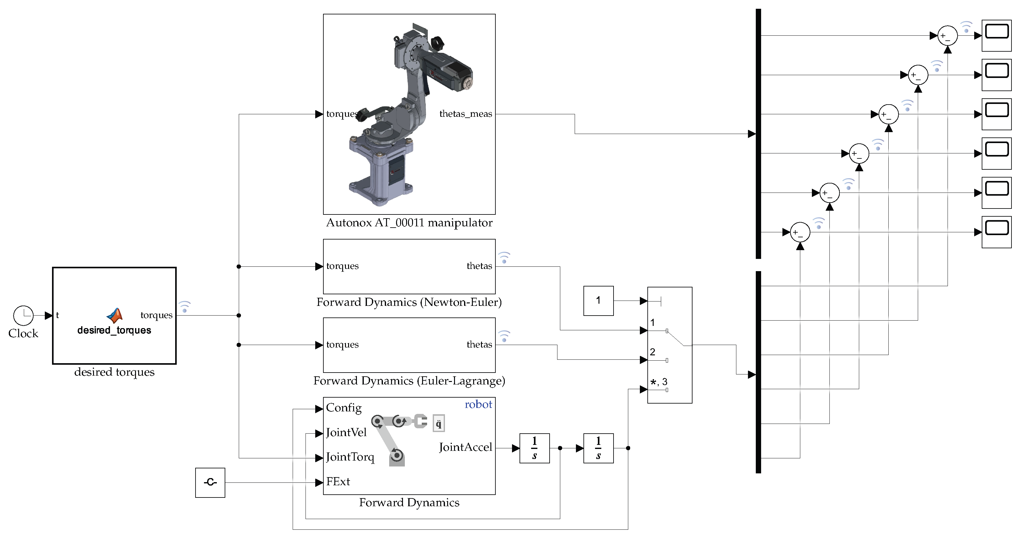
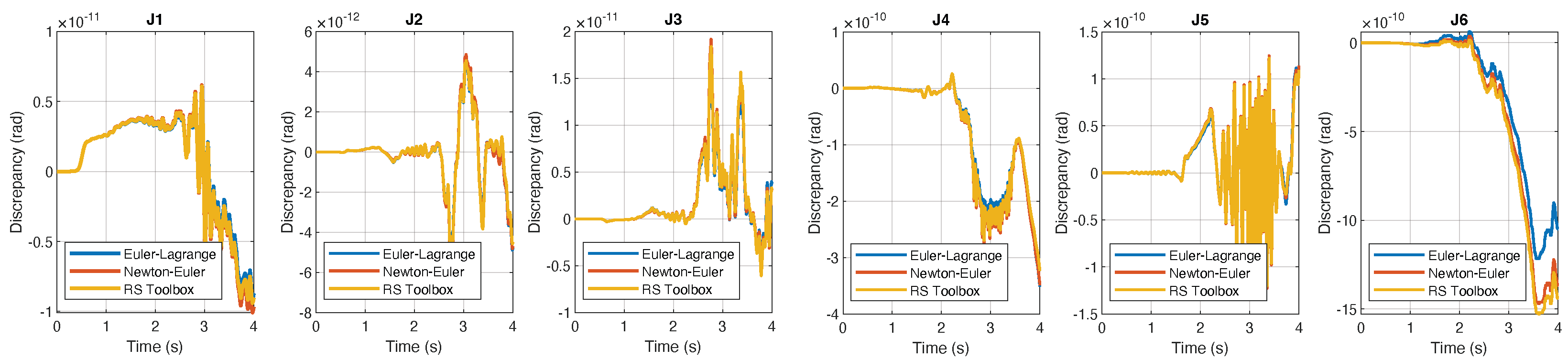
3.3. Simulation of the Forward Dynamics

The dynamic model of the 6 DOF anthropomorphic robot has been derived following both the Euler-Lagrange approach and the Newton-Euler approach, as described in the previous sections. We then compared the results of the Simscape model with those of the mathematical models, to verify the accuracy of the Simscape model. In addition, we extended this comparison to the forward dynamics calculated using the relative Robotic System Toolbox block. We specified a sinusoidal input torque for each joint as:

$${\tau }_i\left(t\right)={\tau }_{0_i}sin\left(t\frac{2\pi }{T}\right)$$

(22)

where ${\tau }_{0_i}=5$ Nm, $T=2 \mathrm{s}$ and the total simulation time was $4 \mathrm{s}$ and then compared the output of the three models. In fact, this test is similar to the one carried out in [9], but in their case the torques came from the inverse dynamics and the forward dynamics was only calculated following the Euler-Lagrange approach. The Simulink scheme used for this comparison is shown in Figure 8, while the discrepancy between the models’ output is reported in Figure 9. Under the act of the same input torque, Figure 9 shows that the responses of the four blocks are closely matched, with errors of the order of ${10}^{-10}$, due to numerical truncations. Therefore, under ideal conditions, the Simscape model can be reliably used instead of mathematical models. This also proves the correctness of the forward dynamics calculated by the Robotics System Toolbox, which does not require an explicit derivation of the robot dynamic model. In addition, the average elapsed time of the simulations using the three different algorithms for the computation of forward dynamics is reported in

Table 3. Elapsed time of the forward dynamics simulation using the three different algorithms.

	Newton-Euler	Euler-Lagrange	Robotics System Toolbox
Average elapsed time	$14.59 \mathrm{s}$	$8.95 \mathrm{s}$	$649.54 \mathrm{s}$

: the elapsed time for the forward dynamics computed through the Euler-Lagrange algorithm is slightly more efficient than the one computed through the Newton-Euler algorithm, while the simulation that uses the Forward Dynamics block provided by the Robotic System Toolbox requires a much longer simulation time than the previous two.

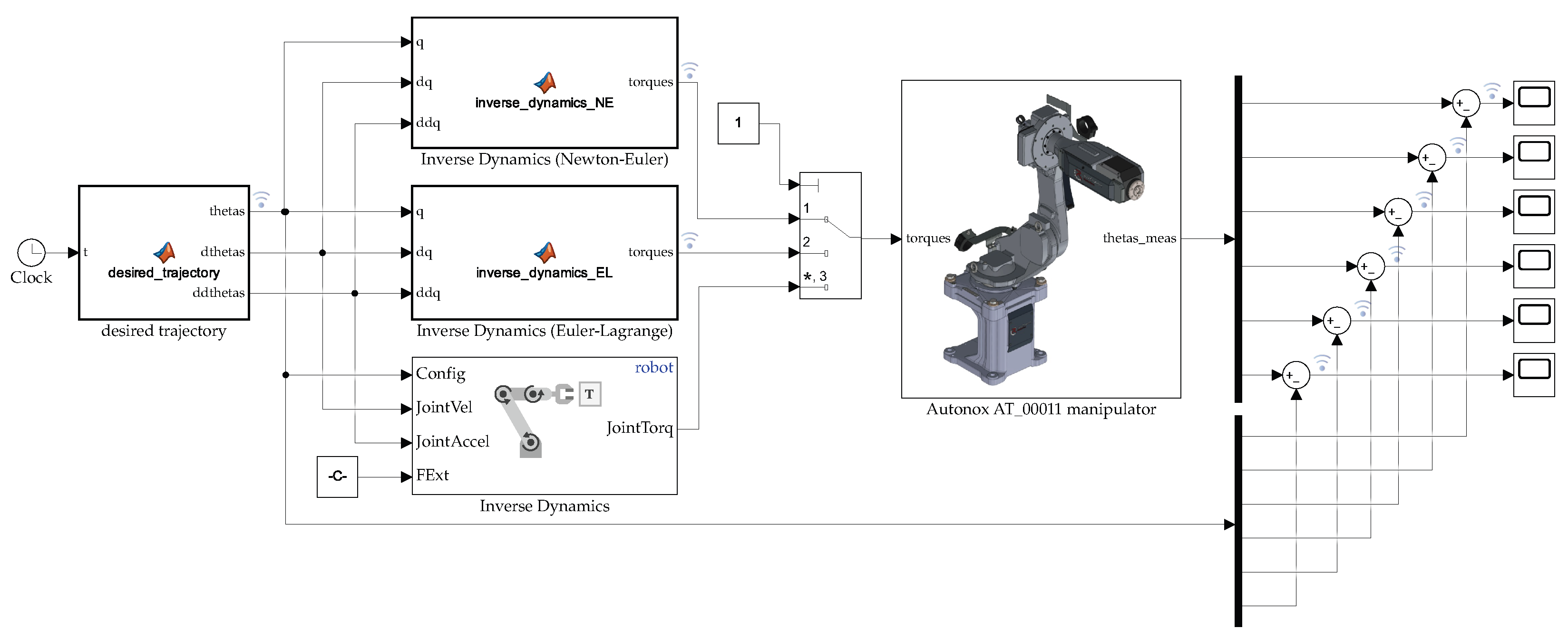
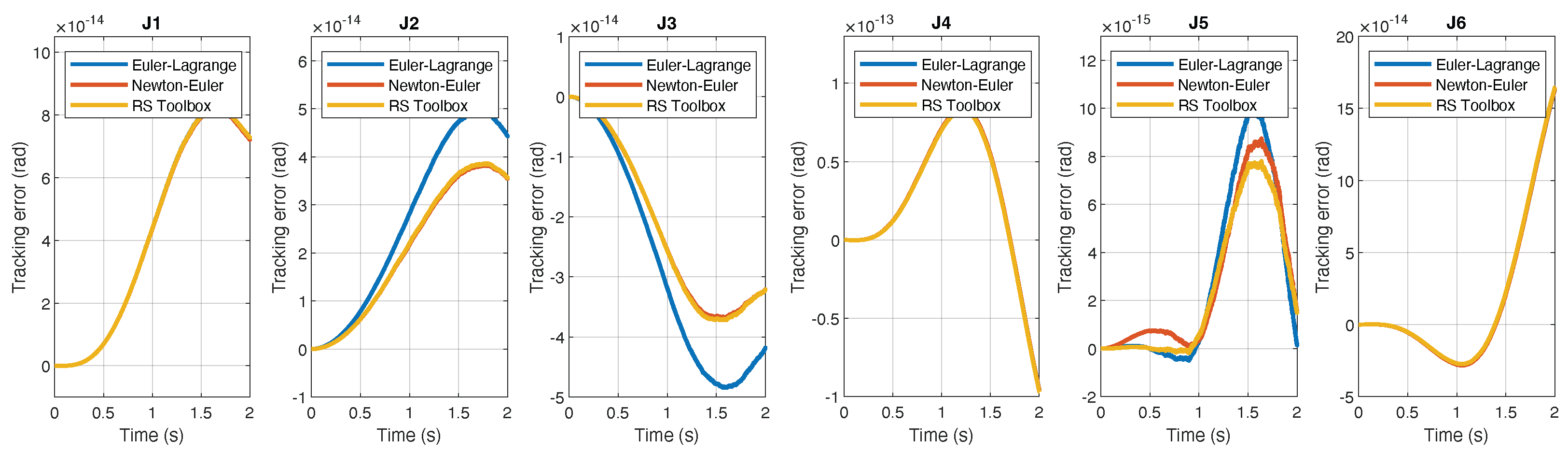
3.4. Inverse Dynamics Control of the Manipulator

After assessing the accuracy of the Simscape model, we implemented a scheme for the inverse dynamics control of the manipulator under ideal conditions. In particular, we defined a trajectory in the joint space, performed inverse dynamics using three different blocks, and provided the computed torques as input to the Simscape model. We then measured the actual joint positions and compared them with the desired ones. The Simulink scheme that we used to perform the inverse dynamics control is shown in Figure 10. For each joint, the desired sinusoidal trajectory is defined as follows:

$${\theta }_i\left(t\right)={\theta }_{i_0}+{\theta }_{i_r}\left[\frac{t-t_0}{T}-\frac{1}{2\pi }sin\left(2\pi \frac{t-t_0}{T}\right)\right],$$

(23)

where ${\theta }_{i_0}$ is the initial joint displacement, ${\theta }_{i_r}$ is the required joint displacement, $t_0$ is the initial time and T is the total time of motion. The initial time is set as $t_0=0 \mathrm{s}$, the total time of motion is set as $T=2 \mathrm{s}$, the initial joint displacement is set as ${\theta }_{i_0}=0^{\circ }$ for each joint while the required joint displacement for each joint is set as ${\theta }_{i_r}={10}^{\circ }$. The resulting trajectory error is shown in Figure 11: the tracking error is on the order of ${10}^{-14}$ and, in the three considered cases, is closely matched. The average elapsed time of the simulations using the three different algorithms for the computation of inverse dynamics is reported in

Table 4. Elapsed timeof the inverse dynamics simulation using the three different algorithms.

	Newton-Euler	Euler-Lagrange	Robotics System Toolbox
Average elapsed time	$4.31 \mathrm{s}$	$4.71 \mathrm{s}$	$177.81 \mathrm{s}$

: the simulations showed, in fact, that the Newton-Euler inverse dynamics is computationally more efficient, while, on the other hand, the use of inverse dynamics block of the Robotic System Toolbox requires a longer simulation time.

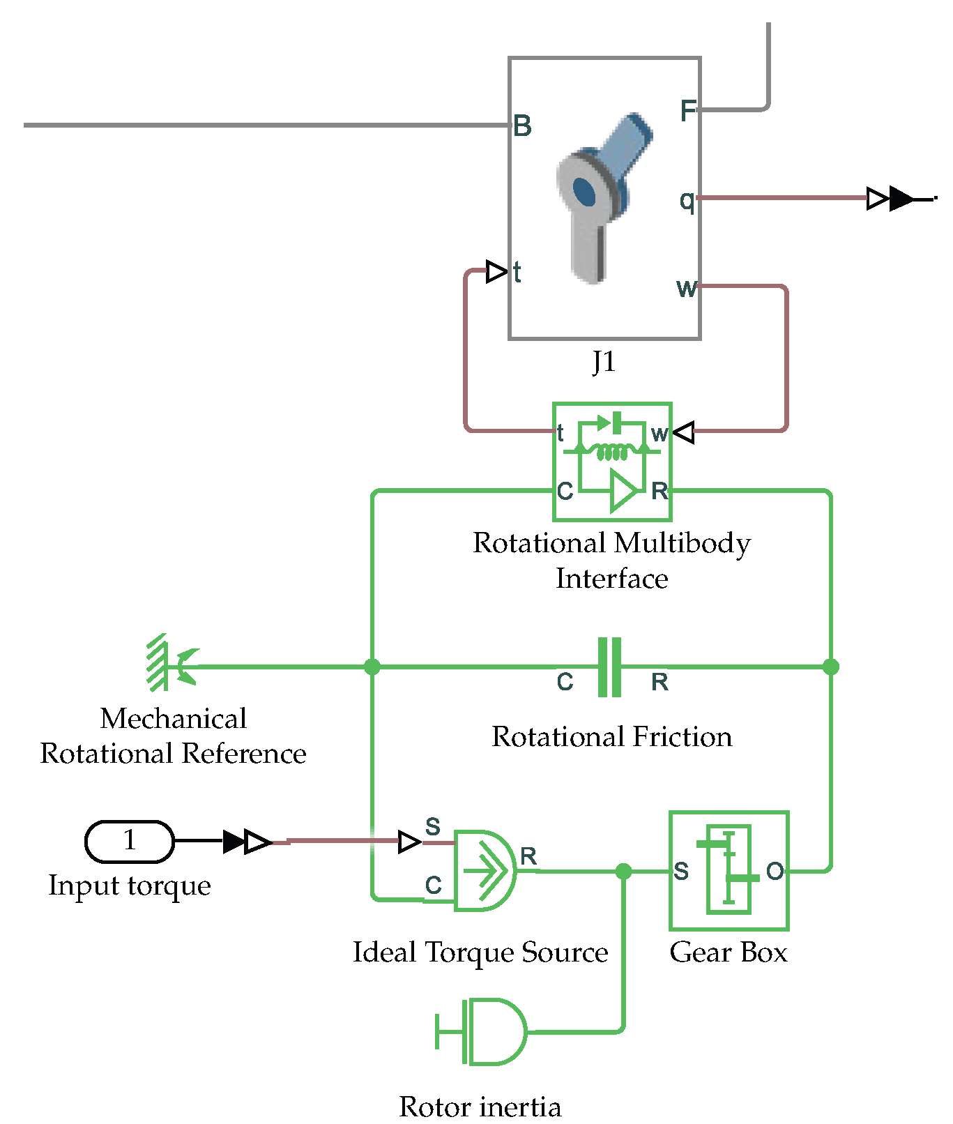
4. Inclusion of Friction, Reduction Gears and Actuators Dynamics

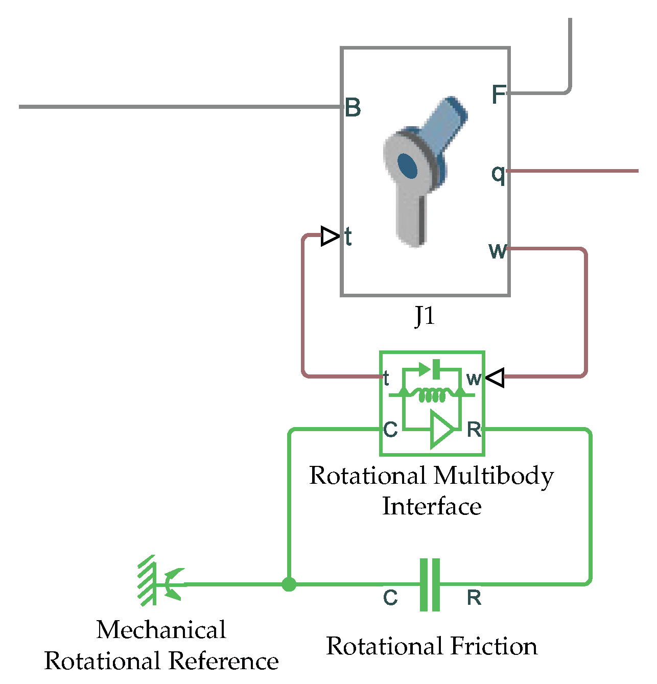
To test robot control strategies, the inclusion of non-idealities such as joint rotational friction, reduction gears and actuators dynamics is of paramount importance. While adding these non-idealities in the mathematical models derived using the Euler-Lagrange or Newton-Euler approach is nontrivial, they can be easily added to the Simscape model.

4.1. Friction

Friction is the result of complex interactions between the surfaces of joints at the microscopic level, and it is rather complex to model [37,38,39]. For this reason, simplified models are typically employed in dynamic modeling of robot joints, the most used being the Lu-Gre model [40]: this model takes into account Coloumb friction $T_C$ (constant at any velocity), viscous friction $T_V$ (directly proportional to the relative velocity), and Stribeck friction $T_S$ (which occurs at low speeds). The sum of Coulomb and Stribeck frictions at the vicinity of zero velocity is often referred to as the breakaway friction $T_{brk}$. However, as Stribeck friction is difficult to model and identify, usually only Coloumb and viscous friction are considered. Taking into account these two dissipative effects, the dynamic model of a manipulator in Equation (5) becomes:

$$\mathit{M}\left(\mathit{\theta }\right)\ddot{\mathit{\theta }}+\mathit{c}(\mathit{\theta },\dot{\mathit{\theta }})+\mathit{g}\left(\mathit{\theta }\right)=\mathit{u}-{\mathit{F}}_C\mathrm{sign}\left(\dot{\mathit{\theta }}\right)-{\mathit{F}}_V\dot{\mathit{\theta }}$$

(24)

where ${\mathit{F}}_C$ and ${\mathit{F}}_V$ are diagonal matrices of Coulomb and Viscous friction parameters. As friction depends on lubrication and temperature, these coefficients depend on operating conditions.

However, friction can be easily included in the Simscape model by expoiting Simscape Fundation Library, as previously done in [9,11]. In particular, a Rotational Friction block can be added to each joint, as in Figure 12. The friction torque is simulated as a function of relative velocity and is assumed to be the sum of the Stribeck, Coulomb, and viscous components, and is approximated by the following equation:

$$T=\sqrt{2e}(T_{brk}-T_C)·exp\left(-\left(\frac{\omega }{{\omega }_{St}}\right)\right)·\frac{\omega }{{\omega }_{St}}+T_C·tanh\left(\frac{\omega }{{\omega }_{Coul}}\right)+f\omega ,$$

(25)

where ${\omega }_{St}$ is the Stribeck velocity threshold, ${\omega }_{Coul}$ is Coulomb velocity threshold and f is the viscous friction coefficient. Both ${\omega }_{St}$ and ${\omega }_{Coul}$ can be derived from the breakaway friction velocity ${\omega }_{brk}$ as:

$${\omega }_{St}={\omega }_{brk}\sqrt{2},{\omega }_{Coul}=\frac{{\omega }_{brk}}{10}.$$

(26)

In fact, the rotational friction block in the Simulink environment requires the definition of only four parameters: the breakaway friction torque $T_{brk}$, the breakaway friction velocity ${\omega }_{brk}$, the Coloumb friction torque $T_C$ and the viscous friction coefficient f. In the Simscape model of the 6 DOF anthropomorphic robot, we added a rotational friction block to every joint, as in Figure 12, specifying the following parameters: $T_{brk}=13$ Nm, ${\omega }_{brk}=0.1$ rad/s, $T_C=10$ Nm and $f=0.001$ Nm/rad.

4.2. Reduction Gears and Motors

Reduction gears are widely used in robotics, as they reduce the speed of the motor and increase its torque. Let us call ${\dot{\theta }}_{mi}$ the angular velocity of the motor that moves the link i (typically mounted on the link $i-1)$, ${\tau }_{m_i}$ its torque produced and $n_{r_i}$ the gear ratio. These quantities are related to the link’s velocity and torque as follows:

$$\left\{\begin{array}{c}{\dot{\theta }}_{m_i}=n_{r_i}{\dot{\theta }}_i\hfill \\ {\tau }_i=n_{r_i}{\tau }_{m_i}\hfill \end{array}\right.$$

(27)

As transmission gears with large reduction ratios are often used in robotics, their presence drastically changes the dynamic model of a robot manipulator in Equation (5). Using the Euler-Lagrange approach, the kinetic energy of motor i, considering only the spin rotor velocity, can be written as:

$${\mathcal{T}}_{m_i}=\frac{1}{2}{I}_{m_i}{\dot{\theta }}_{m_i}^2=\frac{1}{2}{I}_{m_i}{n}_{r_i}^2{\dot{\theta }}_i^2=\frac{1}{2}{B}_{m_i}{\dot{\theta }}_i^2,$$

(28)

where $I_{m_i}$ is the inertia on the motor axis while $B_{m_i}$ is the inertia of the rotor reflected through the reduction ratio. Therefore, the total kinetic energy of the motors is

$${\mathcal{T}}_m=\sum _{i=1}^n{\mathcal{T}}_{m_i}=\frac{1}{2}{\dot{\mathit{\theta }}}^T{\mathit{B}}_m{\dot{\mathit{\theta }}}^{\mathit{T}},$$

(29)

where ${\mathit{B}}_m$ is a diagonal matrix. Including all added terms, the robot dynamics described by Equation (5) can be rewritten as:

$$(\mathit{M}\left(\mathit{\theta }\right)+{\mathit{B}}_m)\ddot{\mathit{\theta }}+\mathit{c}(\mathit{\theta },\dot{\mathit{\theta }})+\mathit{g}\left(\mathit{\theta }\right)+{\mathit{F}}_C\mathrm{sign}\left(\dot{\mathit{\theta }}\right)+{\mathit{F}}_V\dot{\mathit{\theta }}=\mathit{u},$$

(30)

where the inertia matrix $\mathit{M}\left(\mathit{\theta }\right)$ and $\mathit{g}\left(\mathit{\theta }\right)$ are computed including the masses of the motors in the link masses. The dynamic model of the robot can also be written looking from the motor side:

$$\left({\mathit{I}}_m+\mathrm{diag}\left(\frac{m_{ii}\left(\mathit{\theta }\right)}{n_{r_i}^2}\right)\right){\ddot{\mathit{\theta }}}_m+\mathrm{diag}\left(\frac{1}{n_{r_i}}\right)\left(\sum _{j=1}^n{\overline{\mathit{M}}}_j\left(\mathit{\theta }\right){\ddot{\theta }}_j+\mathit{f}(\mathit{\theta },\dot{\mathit{\theta }})\right)={\mathit{\tau }}_m,$$

(31)

where ${\mathit{\tau }}_m$ are the motor torques before reduction gears, ${\overline{\mathit{M}}}_j$ is the jth column of the inertia matrix except the term $m_{ij}$ and

$$\mathit{f}(\mathit{\theta },\dot{\mathit{\theta }})=\mathit{c}(\mathit{\theta },\dot{\mathit{\theta }})+\mathit{g}\left(\mathit{\theta }\right)+{\mathit{F}}_C\mathrm{sign}\left(\dot{\mathit{\theta }}\right)+{\mathit{F}}_V\dot{\mathit{\theta }}.$$

(32)

Equation (31) shows that if the reduction ratios are large, the inertial part of the model becomes almost diagonal. In fact, in industrial practice, robot controllers are typically designed considering only the inertia on the motor side in a decentralized way.

Rotor inertia and transmission gears can be easily added to the Simscape model, as shown in Figure 13. In particular, the gear box block represents an ideal, nonplanetary, fixed gear ratio gear box, while the inertia block can be used to model rotor inertia. Following this approach, we added a gear box to every rotational joint of the our model, specifying the following reduction ratios:

$$\begin{array}{cccccc}\hfill n_{r_1}& =80,\hfill & \hfill n_{r_2}& =50,\hfill & \hfill n_{r_3}& =50,\hfill \\ \hfill n_{r_4}& =30,\hfill & \hfill n_{r_5}& =30,\hfill & \hfill n_{r_6}& =15.\hfill \end{array}$$

(33)

However, we did not use the inertia block, as we modeled the inertia of the motors as described in Section 4.3.

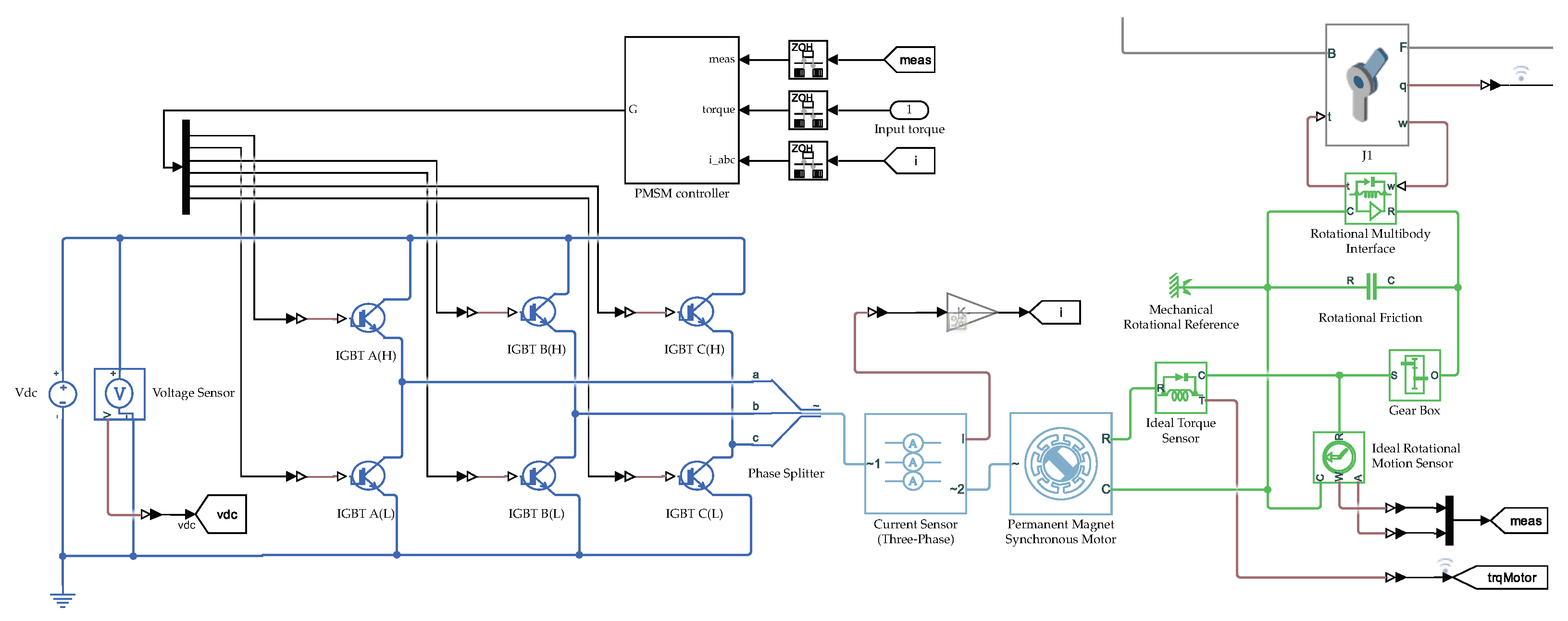
4.3. Actuators Dynamics

Industrial and collaborative robots typically use Permanent Magnets AC Synchronous Motors (PMSMs) for joint control. A detailed robot digital twin should also take into account that motors are not ideal torque generators, but they have their own dynamics (though much faster than the mechanical dynamics) and their saturation limits.

The Simscape Electrical library provides a number of blocks that are particularly useful for the simulation of PMSM motors and three-phase inverters that can be easily added to the Simscape model of the manipulator. However, to the best of our knowledge, no previous study modeled the manipulator’s motors using their scheme provided by Simscape Electrical. In [11] authors modeled the six PMSMs that move the Universal Robot UR5 through their simplified equivalent DC monophase mathematical models, while in [30] brushless DC servomotors were modeled. Figure 14 shows how a PMSM motor can be easily added to the Simscape multibody model. In particular, its whole control scheme, which computes the three-phase inverter IGBTs inputs, can be simulated: this allows to comprehensively simulate the control of the actuators. In addition, PMSM Simulink block also allows to specify the inertia of the rotor.

In our Simscape model, we modeled each joint as in Figure 14 and the input torque of the PMSMs controller is the commanded torque of the manipulator’s control algorithm. It is worth mentioning that if we want to fully take into account the actuators dynamics in the Simscape model, the Simulink solver configuration should be adjusted according to the PWM switching frequency and motor control sample time.

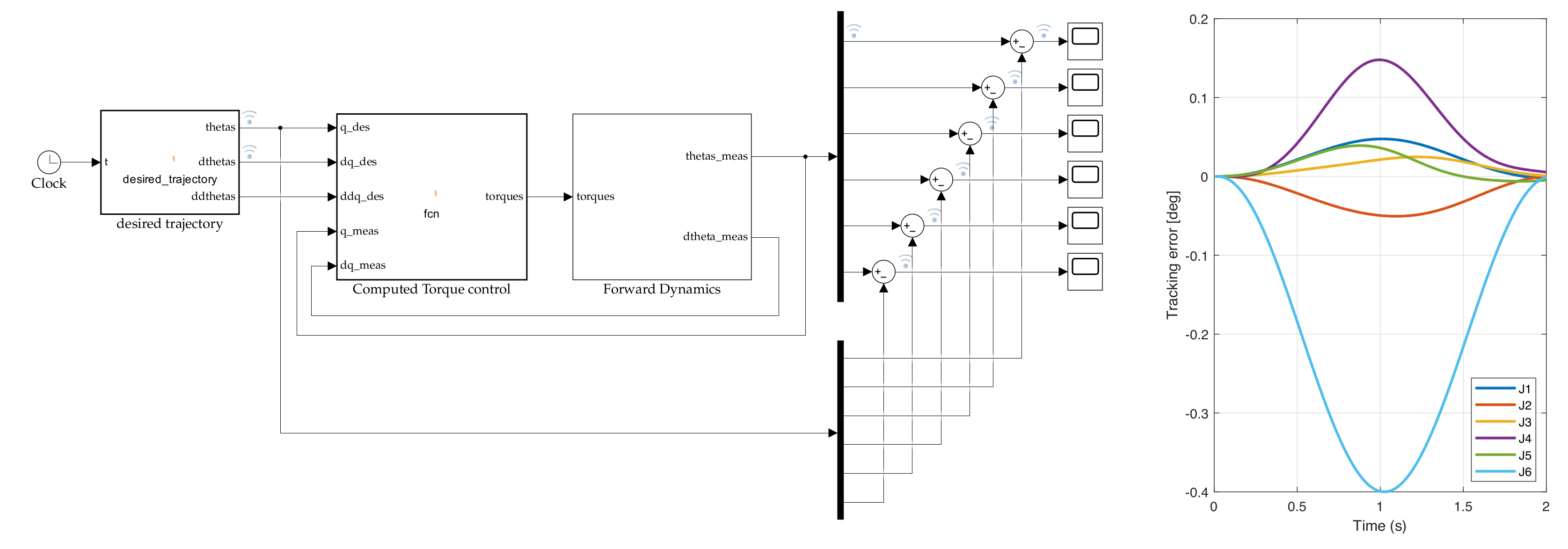
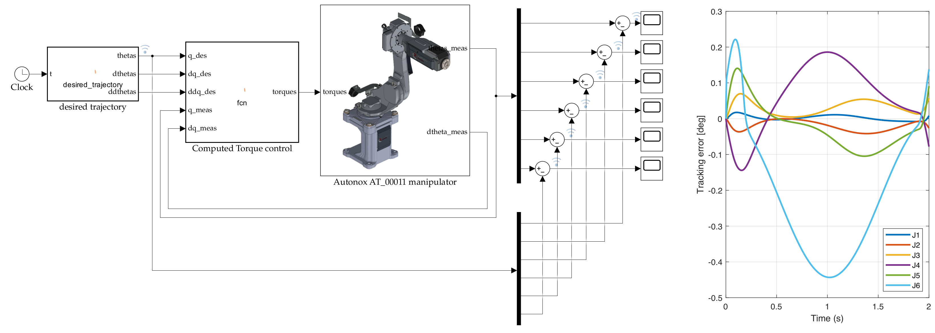
5. Simulation of a Computed Torque Control Scheme

Finally, we used the Simscape robot model with joint friction, reduction gears, and actuator dynamics to test a computed torque control scheme [41,42]. In addition, we compared the result obtained with the Simscape model with those obtained using the mathematical model described by Equation (5), under the same input torques.

Following the well-known computed control scheme (often referred to as feedback linearization), the input torque is calculated as:

$$\mathit{\tau }=\mathrm{diag}\left(\frac{1}{n_{r_i}}\right)\mathit{M}\left({\mathit{\theta }}_{me}\right)\left[{\ddot{\mathit{\theta }}}_d+{\mathit{K}}_P\left({\mathit{\theta }}_d-{\mathit{\theta }}_{me}\right)+{\mathit{K}}_D\left({\dot{\mathit{\theta }}}_d-{\dot{\mathit{\theta }}}_{me}\right)\right]+\mathrm{diag}\left(\frac{1}{n_{r_i}}\right)\mathit{f}({\mathit{\theta }}_{me},{\dot{\mathit{\theta }}}_{\mathit{me}})$$

(34)

where ${\mathit{\theta }}_{me}$ are the measured joint positions, ${\dot{\mathit{\theta }}}_{me}$ are the measured joint velocities (typically estimated by numerical differentiation of the encoder measurements), ${\mathit{\theta }}_d$ are the desired joint positions, ${\dot{\mathit{\theta }}}_d$ are the desired joint velocities and ${\ddot{\mathit{\theta }}}_d$ are the desired joint accelerations. In addition, ${\mathit{K}}_P$ and ${\mathit{K}}_D$ are the diagonal proportional and derivative gain matrices: global stabilization is ensured for any positive definite ${\mathit{K}}_P$ and ${\mathit{K}}_D$, provided that the dynamic parameters of the robot are accurately known [32].

The Simulink scheme of the computed torque algorithm implemented is shown on the left in Figure 15 and Figure 16. More in detail, we specified a sinusoidal trajectory for each joint as in Equation (23), where ${\theta }_{i_0}=0^{\circ }$ for each joint, $t_0=0$ s, $T=2$ s and:

$$\begin{array}{cccccc}\hfill {\theta }_{1_r}& ={90}^{\circ },\hfill & \hfill {\theta }_{2_r}& =-{90}^{\circ },\hfill & \hfill {\theta }_{3_r}& ={30}^{\circ },\hfill \\ \hfill {\theta }_{4_r}& =-{90}^{\circ },\hfill & \hfill {\theta }_{5_r}& ={90}^{\circ },\hfill & \hfill {\theta }_{6_r}& ={90}^{\circ }.\hfill \end{array}$$

(35)

PD gains are usually selected for critical damping ($\epsilon =1$): in this case $K_{P_i}={\omega }_{n_i}^2$ and $K_{D_i}=2\sqrt{K_{P_i}}$, where ${\omega }_{n_i}$ is the natural frequency of joint error i. In our model, after some iterations, we selected the following gain matrices:

$${\mathit{K}}_P=\mathrm{diag}\left(100\right),{\mathit{K}}_D=\mathrm{diag}\left(20\right).$$

(36)

The resulting tracking error for each joint is shown on the right in Figure 15 and Figure 16. Even though the tracking error of the two models is similar, the Simscape model includes a more complex friction model and PMSMs dynamics, which results in a higher tracking error at the beginning and at the end of the motion (where the velocity is close to zero). These simulations prove that the Simscape model can be efficiently employed to test control strategies more reliably, as it is easier to include complex models of non-idealities.

6. Conclusions

In this work, we presented the design of high-fidelity digital twins of robots using Simscape Multibody. In particular, we first created a model of a six DOF articulated robot under ideal conditions and then compared the output of the Simscape model with the dynamic mathematical model of the manipulator (derived using both the Euler-Lagrange and Newton-Euler approach), proving its accuracy. We also used the Simscape model in conjunction with the well-established Robotic System Toolbox to assess its capabilities: even though this toolbox allows performing kinematic and dynamic robotic simulations without requiring advanced robotic knowledge, its use significantly slows down the simulation. Subsequently, we added non-idealities to the model, including joint rotational friction, transmission gears, and actuator dynamics, exploiting other Simscape libraries, such as Simscape Electrical to model PMSM motors. The resulting high-fidelity robot model can be reliably used in simulations with different objectives, such as designing and testing different control strategies, generating data for learning-based approaches, and optimizing power consumption. Here, we expolited the Simscape model to test a computed torque control scheme. Future works should aim to include additional non-idealities, such as flexibility introduced by belts and harmonic drives.

References

1. Garg, G.; Kuts, V.; Anbarjafari, G. Digital twin for fanuc robots: Industrial robot programming and simulation using virtual reality. Sustainability 2021, 13, 336. [Google Scholar] [CrossRef]
2. Automation Control Environment (ACE) Version 4 User Manual. Available online: https://assets.omron.eu/downloads/manual/en/v4/i633_ace_4.0_users_manual_en.pdf (accessed on 29 February 2024).
3. Borangiu, T.; Răileanu, S.; Anton, F.; Lențoiu, I.; Negoiță, R. Cloud-Based Digital Twin for Robot Health Monitoring and Integration in Cyber-Physical Production Systems. Mech. Mach. Sci. 2023, 127, 261–269. [Google Scholar] [CrossRef]
4. Connolly, C. Technology and applications of ABB RobotStudio. Ind. Robot 2009, 36, 540–545. [Google Scholar] [CrossRef]
5. Kaczmarek, W.; Panasiuk, J.; Borys, S.; Banach, P. Industrial robot control by means of gestures and voice commands in off-line and on-line mode. Sensors 2020, 20, 6358. [Google Scholar] [CrossRef] [PubMed]
6. Collins, J.; Chand, S.; Vanderkop, A.; Howard, D. A review of physics simulators for robotic applications. IEEE Access 2021, 9, 51416–51431. [Google Scholar] [CrossRef]
7. Simscape Multibody. Available online: https://www.mathworks.com/products/simscape-multibody.html (accessed on 29 February 2024).
8. Robotic System Toolbox. Available online: https://www.mathworks.com/products/robotics.html (accessed on 29 February 2024).
9. Truc, L.N.; Lam, N.T. Quasi-physical modeling of robot IRB 120 using Simscape Multibody for dynamic and control simulation. Turk. J. Electr. Eng. Comput. Sci. 2020, 28, 1949–1964. [Google Scholar] [CrossRef]
10. Truc, L.N.; Quang, N.P.; Quang, N.H. Impact analysis of actuator torque degradation on the IRB 120 robot performance using simscape-based model. Int. J. Electr. Comput. Eng. 2021, 11, 4850–4864. [Google Scholar] [CrossRef]
11. Raviola, A.; Guida, R.; Bertolino, A.C.; De Martin, A.; Mauro, S.; Sorli, M. A Comprehensive Multibody Model of a Collaborative Robot to Support Model-Based Health Management. Robotics 2023, 12, 71. [Google Scholar] [CrossRef]
12. Gouasmi, M.; Ouali, M.; Fernini, B.; Meghatria, M. Kinematic modelling and simulation of a 2-R robot using solidworks and verification by matlab/simulink. Int. J. Adv. Robot. Syst. 2012, 9, 245. [Google Scholar] [CrossRef]
13. Ibrahim, B.; Zargoun, A.M. Modelling and control of SCARA manipulator. Procedia Comput. Sci. 2014, 42, 106–113. [Google Scholar] [CrossRef]
14. Zhang, Z.; Zhang, C.; Deng, Z.; Feng, H. Modelling and Dynamic Simulation of Palletizing Robot System Based on Multibody. In Proceedings of the 2023 IEEE 6th Information Technology, Networking, Electronic and Automation Control Conference (ITNEC), Chongqing, China, 24–26 February 2023; pp. 583–587. [Google Scholar] [CrossRef]
15. Lee, K.; Lee, J.; Woo, B.; Lee, J.; Lee, Y.J.; Ra, S. Modeling and Control of a Articulated Robot Arm with Embedded Joint Actuators. In Proceedings of the 2018 International Conference on Information and Communication Technology Robotics (ICT-ROBOT), Busan, Republic of Korea, 6–8 September 2018. [Google Scholar] [CrossRef]
16. Bârsan, A.; Racz, S.G.; Breaz, R.; Crenganiș, M. Dynamic analysis of a robot-based incremental sheet forming using Matlab-Simulink Simscape™ environment. Mater. Today Proc. 2022, 62, 2538–2542. [Google Scholar] [CrossRef]
17. Racz, S.G.; Crenganiș, M.; Breaz, R.E.; Bârsan, A.; Gîrjob, C.E.; Biriș, C.M.; Tera, M. Integrating Trajectory Planning with Kinematic Analysis and Joint Torques Estimation for an Industrial Robot Used in Incremental Forming Operations. Machines 2022, 10, 531. [Google Scholar] [CrossRef]
18. Olaya, J.; Pintor, N.; Avilés, O.F.; Chaparro, J. Analysis of 3 RPS robotic platform motion in simscape and MATLAB GUI environment. Int. J. Appl. Eng. Res. 2017, 12, 1460–1468. [Google Scholar]
19. Noskievic, P.; Walica, D. Design and Realisation of the Simulation Model of the Stewart Platform using the MATLAB-Simulink and the Simscape Multibody Library. In Proceedings of the 2020 21th International Carpathian Control Conference (ICCC), High Tatras, Slovakia, 27–29 October 2020. [Google Scholar] [CrossRef]
20. Khnissi, K.; Jabeur, C.B.; Seddik, H. 3D Simulator for Navigation of a Mobile Robot Using Simscape-SIMULINK. In Proceedings of the 2019 International Conference on Control, Automation and Diagnosis (ICCAD), Grenoble, France, 2–4 July 2019. [Google Scholar] [CrossRef]
21. Siwek, M.; Baranowski, L.; Panasiuk, J.; Kaczmarek, W. Modeling and simulation of movement of dispersed group of mobile robots using Simscape multibody software. AIP Conf. Proc. 2019, 2078, 020045. [Google Scholar] [CrossRef]
22. Eldirdiry, O.; Zaier, R. Modeling biomechanical legs with toe-joint using simscape. In Proceedings of the 2018 11th International Symposium on Mechatronics and its Applications (ISMA), Sharjah, United Arab Emirates, 4–6 March 2018; pp. 1–7. [Google Scholar] [CrossRef]
23. Aldair, A.A.; Al-Mayyahi, A.; Jasim, B.H. Control of Eight-Leg Walking Robot Using Fuzzy Technique Based on SimScape Multibody Toolbox. Mater. Sci. Eng. 2020, 745, 012015. [Google Scholar] [CrossRef]
24. Nguyen, N.T.; Nguyen, T.N.T.; Tong, H.N.; Truong, H.V.A.; Tran, D.T. Dynamic Parameter Identification based on the Least Squares method for a 6-DOF Manipulator. In Proceedings of the 2023 International Conference on System Science and Engineering (ICSSE), Ho Chi Minh, Vietnam, 27–28 July 2023; pp. 301–305. [Google Scholar] [CrossRef]
25. Du, N.; Yan, L.; Gao, X.; Xiang, P.; Bu, S. Simulation Analysis of Discrete Admittance Control of Manipulator. In Proceedings of the 2022 IEEE 17th Conference on Industrial Electronics and Applications (ICIEA), Chengdu, China, 16–19 December 2022; pp. 926–930. [Google Scholar] [CrossRef]
26. Truc, L.N.; Vu, L.A.; Thoan, T.V.; Thanh, B.T.; Nguyen, T.L. Adaptive Sliding Mode Control Anticipating Proportional Degradation of Actuator Torque in Uncertain Serial Industrial Robots. Symmetry 2022, 14, 957. [Google Scholar] [CrossRef]
27. Nguyen, V.C.; Thi, H.L.; Nguyen, T.L. A Lyapunov-based model predictive control strategy with a disturbances compensation mechanism for dual-arm manipulators. Eur. J. Control 2023, 75, 100913. [Google Scholar] [CrossRef]
28. Othman, Z.H.; Mahfouz, D.M.; Shehata, O.M. Analysis and Development of a Hybrid Position/Force Control for a N-DoF Robotic Manipulator. In Proceedings of the 2022 4th Novel Intelligent and Leading Emerging Sciences Conference (NILES), Giza, Egypt, 22–24 October 2022; pp. 90–94. [Google Scholar] [CrossRef]
29. Pozzi, M.; Achilli, G.M.; Valigi, M.C.; Malvezzi, M. Modeling and Simulation of Robotic Grasping in Simulink Through Simscape Multibody. Front. Robot. AI 2022, 9, 873558. [Google Scholar] [CrossRef] [PubMed]
30. Grazioso, S.; Di Maio, M.; Di Gironimo, G. Conceptual design, control, and simulation of a 5-DoF robotic manipulator for direct additive manufacturing on the internal surface of radome systems. Int. J. Adv. Manuf. Technol. 2019, 101, 2027–2036. [Google Scholar] [CrossRef]
31. Craig, J.J. Introduction to Robotics: Mechanics and Control, 2nd ed.; Addison-Wesley Longman Publishing Co., Inc.: Upper Saddle River, NJ, USA, 1989. [Google Scholar]
32. Siciliano, B.; Sciavicco, L.; Villani, L.; Oriolo, G. Robotics: Modelling, Planning and Control, 3rd ed.; Springer: London, UK, 2009. [Google Scholar]
33. Autonox Robotics GmbH. Available online: https://www.autonox.com/en (accessed on 29 February 2024).
34. Denavit, J.; Hartenberg, R. A Kinematic Notation for Lower-Pair Mechanisms Based on Matrices. J. Appl. Mech. Trans. ASME 1955, 22, 215–221. [Google Scholar] [CrossRef]
35. de Jalón, J.; Bayo, E. Kinematic and Dynamic Simulation of Multibody Systems: The Real-Time Challenge; Mechanical Engineering Series; Springer: Berlin/Heidelberg, Germany, 1994. [Google Scholar]
36. Corke, P.I. A robotics toolbox for MATLAB. IEEE Robot. Autom. Mag. 1996, 3, 24–32. [Google Scholar] [CrossRef]
37. Bittencourt, A.C.; Gunnarsson, S. Static friction in a robot joint-modeling and identification of load and temperature effects. J. Dyn. Syst. Meas. Control. Trans. ASME 2012, 134, 051013. [Google Scholar] [CrossRef]
38. Zhang, L.; Wang, J.; Chen, J.; Chen, K.; Lin, B.; Xu, F. Dynamic modeling for a 6-DOF robot manipulator based on a centrosymmetric static friction model and whale genetic optimization algorithm. Adv. Eng. Softw. 2019, 135, 102684. [Google Scholar] [CrossRef]
39. Bittencourt, A.C.; Wernholt, E.; Sander-Tavallaey, S.; Brogårdh, T. An extended friction model to capture load and temperature effects in robot joints. In Proceedings of the 2010 IEEE/RSJ International Conference on Intelligent Robots and Systems, Taipei, Taiwan, 18–22 October 2010; pp. 6161–6167. [Google Scholar] [CrossRef]
40. Haessig, D.; Friedland, B. On the modeling and simulation of friction. J. Dyn. Syst. Meas. Control. Trans. ASME 1991, 113, 354–362. [Google Scholar] [CrossRef]
41. Falkenhahn, V.; Hildebrandt, A.; Neumann, R.; Sawodny, O. Model-based feedforward position control of constant curvature continuum robots using feedback linearization. In Proceedings of the 2015 IEEE International Conference on Robotics and Automation (ICRA), Seattle, WA, USA, 26–30 May 2015; pp. 762–767. [Google Scholar] [CrossRef]
42. Kali, Y.; Saad, M.; Benjelloun, K. Optimal super-twisting algorithm with time delay estimation for robot manipulators based on feedback linearization. Robot. Auton. Syst. 2018, 108, 87–99. [Google Scholar] [CrossRef]
Figure 1. 6 DOF anthropomorphic robot with attached DH frames.
Robotics 13 00062 g001
Figure 2. Simscape Multibody model of the 6 DOF anthropomorphic robot.
Robotics 13 00062 g002
Figure 3. (left) Subsystem of each link that composes the 6 DOF anthropomorphic robot and (right) 3D visualization of the manipulator generated by Simscape Multibody.
Robotics 13 00062 g003
Figure 4. Kinematic control of the manipulator using user-defined Matlab functions.
Robotics 13 00062 g004
Figure 5. Kinematiccontrol of the manipulator robot using Robotic System Toolbox functions.
Robotics 13 00062 g005
Figure 6. Measuredjoint positions and velocities during the kinematic control of the manipulator though user-defined Matlab functions.
Robotics 13 00062 g006
Figure 7. Measuredjoint positions and velocities during the kinematic control of the manipulator though Robotic System Toolbox blocks.
Robotics 13 00062 g007
Figure 8. Simulink scheme of the forward dynamics of the manipulator using the Simscape Multibody model, the Newton-Euler model, the Euler-Lagrange model and the Robotics System Toolbox block.
Robotics 13 00062 g008
Figure 9. Discrepancy between the output of the Simulink Multibody model, the Newton-Euler or Euler-Lagrange model and the Robotics System Toolbox block.
Robotics 13 00062 g009
Figure 10. Inverse dynamics control of the manipulator using user-defined Matlab functions or the inverse dynamics block provided by Robotic System Toolbox.
Robotics 13 00062 g010
Figure 11. Trajectory tracking error for each joint when the manipulator is controlled through inverse dynamics in Simscape Multibody.
Robotics 13 00062 g011
Figure 12. Simscape multibody revolute joint with rotational friction.
Robotics 13 00062 g012
Figure 13. Torque-controlled Simscape multibody revolute joint with rotational friction, reduction gear and rotor inertia.
Robotics 13 00062 g013
Figure 14. Simscapemultibody revolute joint with rotational friction, reduction gear and PMSM motor.
Robotics 13 00062 g014
Figure 15. (left) Simulation of a computed torque scheme using the robot’s mathematical model (including reduction gears, viscous and Coulomb friction) and (right) resulting tracking error for each joint.
Robotics 13 00062 g015
Figure 16. (left) Simulation of a computed torque scheme using the Simscape model (including reduction gears, a complete model of friction and actuators dynamics) and (right) resulting tracking error for each joint.
Robotics 13 00062 g016