Continuous Online Semantic Implicit Representation for Autonomous Ground Robot Navigation in Unstructured Environments

Abstract

While mobile ground robots have now the physical capacity of travelling in unstructured challenging environments such as extraterrestrial surfaces or devastated terrains, their safe and efficient autonomous navigation has yet to be improved before entrusting them with complex unsupervised missions in such conditions. Recent advances in machine learning applied to semantic scene understanding and environment representations, coupled with modern embedded computational means and sensors hold promising potential in this matter. This paper therefore introduces the combination of semantic understanding, continuous implicit environment representation and smooth informed path-planning in a new method named COSMAu-Nav. It is specifically dedicated to autonomous ground robot navigation in unstructured environments and adaptable for embedded, real-time usage without requiring any form of telecommunication. Data clustering and Gaussian processes are employed to perform online regression of the environment topography, occupancy and terrain traversability from 3D semantic point clouds while providing an uncertainty modeling. The continuous and differentiable properties of Gaussian processes allow gradient based optimisation to be used for smooth local path-planning with respect to the terrain properties. The proposed pipeline has been evaluated and compared with two reference 3D semantic mapping methods in terms of quality of representation under localisation and semantic segmentation uncertainty using a Gazebo simulation, derived from the 3DRMS dataset. Its computational requirements have been evaluated using the Rellis-3D real world dataset. It has been implemented on a real ground robot and successfully employed for its autonomous navigation in a previously unknown outdoor environment.

1. Introduction

Navigation of autonomous vehicles has been the subject of growing interest since the development of self-driving cars and robots for various applications from industrial logistics to extraterrestrial exploration. The robot capacities as well as the context and goal of its navigation greatly affects the development and choice of methods to efficiently guide it towards its objective. The work presented in this paper focuses on the domain of ground robot navigation in unknown and unstructured outdoor environments. In this context, autonomous robots should rely only on their embedded sensors to perceive the surroundings in order to build a model allowing to navigate. While most existing methods performing robot navigation from sensor measurements rely solely on geometric information, recent advances in the domain showed that the inclusion of the semantic understanding of the environment can greatly improve the robot navigation safety and efficiency. In the given context, semantic understanding can be seen as the ability to densely label sensor data with semantic classes (e.g., types of objects or terrains) and to exploit this labeling to extract valuable information. Previously developed methods usually rely on explicit discrete 3D mapping as an intermediate representation between sensor measurements and the navigation space. While this has the advantage of producing a visualisation of the navigated environment to a remote operator, it constrains the navigation space to be derived from this visual representation. Moreover, the discrete aspect of the mapping process introduces limitations on navigation flexibility and completeness as their employment for such tasks implicates a trade-off between resolution and computation costs in addition to the fact that their design does not directly allow to perform requests and optimisation for smooth informed planning. Finally, the growing availability of modern and powerful computational means such as GPUs and TPUs can allow algorithms and methods that were previously considered unpractical for online embedded usage on a ground robot.

In an effort to tackle current limitations, we introduce the COSMAu-Nav (Continuous Online Semantic iMplicit representation for Autonomous Navigation) method, which combines modern computational means for UGV navigation in unstructured environments by the use of semantic segmentation, implicit continuous representation of the navigation space in the form of Gaussian process Regression (GPR) and gradient based optimisation for smooth path-planning. The computation of navigation-relevant variables from semantic 3D point clouds and their compression and fusion before integration make it possible to build a continuous and differentiable implicit environment representation with lighter storage requirements. Two different algorithms for data compression and fusion are proposed and compared: a grid-based clustering algorithm and a two-step k-means clustering algorithm. The resulting regression and associated uncertainty modeling can then be exploited for informative robot navigation. Its continuous and differentiable properties have been leveraged to perform smooth path planning using gradient descent Bézier curve optimisation from a coarse prior path computed with the T-RRT [1] sampling based planner.

A previously developed modular semantic mapping and navigation ROS architecture [2] named SMaNA (Semantic Mapping and Navigation Architecture) has been used as reference to compare mapping accuracy and computational performances. The advantages of this new methodology are highlighted through the evaluation of the resulting GPR environment representation and its comparison against two commonly-used 3D semantic mapping methods integrated in SMaNA in a simulated Gazebo (https://gazebosim.org, accessed on 1 May 2024) environment built from the 3DRMS dataset [3]. Computational and memory requirements have been compared using the Rellis-3D real-world dataset [4]. The COSMAu-Nav architecture has been implemented on board a real mobile ground robot to perform a navigation mission in an outdoor environment.

Related work and the main contributions are given in Section 2. Section 3 describes a new methodology for GPR environment representation, which is exploited by the proposed COSMAu-Nav architecture for smooth path-planning in Section 4. Section 5 presents the comparative evaluations in the simulated environment and real-world dataset with respect to the SMaNA architecture. Section 6 describes COSMAu-Nav implementation onboard a ground robot, its adaptation for a global navigation mission and experimental results.

2. Related Work

In line with the objectives of this work, this section describes existing methods for online mapping from embedded sensor data, employed for robot navigation. The main characteristics of the most representative methods, with respect to identified application requirements, are summarized in

Table 1. Comparative study of online robot mapping and navigation methods (MLG: Multi-Layer Grid, MLP: Multi-Layer Perceptron).

Method	Navigation Structure	Intermediate Representation	Representation Storage	Domain	Scale	Employ Semantics	Uncertainty Measurement
Wermelinger et al. [5]	2D MLG	Ø	Ø	Discrete	Global	no	no
SMaNA [2] with [6]	2D MLG	Octomap	Explicit	Discrete	Global	yes	no
SMaNA [2] with [7]	2D MLG	TSDF	Semi-Implicit	Discrete	Global	yes	no
Maturna et al. [8]	2D MLG	Ø	Ø	Discrete	Local	yes	yes
Ewen et al. [9]	2.5D Triangle Mesh	Ø	Ø	Discrete	Local	yes	no
Sznaier et al. [10]	Sampled SDF	Local MLPs	Implicit	Continuous	Global	no	no
Ghaffari et al. [11]	2D MLG	GPR	Implicit	Continuous	Global	no	yes
Morelli et al. [12]	Sampled 2D Graph	Hilbert Map	Implicit	Continuous	Global	no	no
COSMAu-Nav (ours)	GPR	Compressed Points	Implicit	Continuous	Hybrid	yes	yes

and compared to our proposed solution. These characteristics are the following:

• The presence and nature of an intermediate representation between sensor data and navigation structure, which impacts scalability and computational performances.
• The continuous or discrete aspect of the navigation structure, which defines the characteristics and modalities of the planning methods that can be applied.
• Whether it can be applied to large scale navigation tasks or for local planning.
• Whether semantics are employed to enrich the environment understanding and improve navigation.
• Whether an uncertainty measurement is provided, which we consider a key aspect to guarantee robot safety.

2.1. Semantic Mapping for Robot Navigation

Geometric mapping methods have been proven successful to guide robots through challenging environments [5,13] and developments are still pursued in the domain such as in [14,15]. Nonetheless, complex outdoor environments are populated with various types of terrain with different properties in terms of mobile robot locomotion, which cannot be efficiently classified using geometrical information alone. In the past years, several reliable and fast semantic segmentation of images and point clouds have been made available thanks to the continuous improvement of neural networks, e.g., [16,17]. The growing interest of the community for the inclusion of semantics in the environment representation for navigation suggests that it can greatly improve safety and efficiency, notably while navigating in unstructured environments [18]. The adaptation of existing mapping methods to include semantic information, such as Octomap in [6] and TSDF in [7], has shown improvement in the quality and usability of robot mapping as well as in SLAM [19], human-robot interaction and navigation in structured environments [20]. In [2,21], the Octomap and TSDF semantic mapping methods have been interfaced to build a global 2D multi-layer grid on which A* path-planning weighted by terrain classes traversability factors can be performed. A combination of semantic Octrees, 2D multi-layered grids and semantic classes traversability factor association to perform legged robot motion planning on natural terrains has also been presented in [22]. However, all these methods rely on a discrete and explicit mapping representation as the interface between the robot perception and navigation layers, which presents inherent limitations in terms of flexibility, computational efficiency and memory usage. As an alternative, the direct integration of measurements in a navigation structure has been studied. In [8,23], the semantic segmentation of embedded camera images is projected onto an horizontal 2D plane with an associated traversability coefficient, then a fusion of these observations produces a sliding robot-centered 2.5D traversability grid which can be used by path planning algorithms. In [9], a robot-centered surface mesh enriched with semantic labels and a study of friction coefficients between legged-robot feet and different terrains has been proposed, where height and labels of the mesh elements were allocated using Bayesian fusion. While these methods offer significant computational cost reduction, the direct projection of measurements in a grid or a mesh still limits the accuracy and prediction capability of these local representations for navigation purposes.

2.2. Implicit Representations for Robot Navigation

In order to tackle the limitations highlighted in the previous section, implicit representations have been studied as the interface between robotic perception and navigation. Methods based on Deep learning allow to produce such implicit scene representation, lighter to store than raw data or explicit representations while capturing the scene accurately and allowing to make predictions for reconstruction completion. Multi-layer perceptrons (MLP) were used for occupancy modelling in [10]. Neural Radiance Fields (NeRFs [24]) are able to produce high quality and realistic 3D reconstructions, however their training and rendering requires heavy computation and cannot be performed online. An adaptation of NeRFs presented in [25] and the Gaussian splatting methodology presented in [26] have demonstrated the ability to render radiance fields online, however their online training still remains cumbersome. Implicit Mapping and Positioning (IMAP [27]) is able to reconstruct scenes in real time, but its application is yet limited in scale. Statistical Regression methods require less computational requirements and can thus attain better scalability. In this category, Bayesian regression functions known as Hilbert maps [28] perform regression of sparse sensor data and are one of the first implicit representation methods used for mapping a robot space for large-scale navigation [12]. This category of methods is mostly adapted to binary classification and does not provide a confidence measure, which prevents their usage for uncertainty-aware navigation.

Gaussian process regression (GPR), which yields a variance of the resulting inference, has been applied for robot mapping e.g., in [11,29]. A drawback is the cubical scaling of their computational cost with the number of training points. Their real-time usage thus requires sensor data compression before training. In [30], sparse pseudo-points capturing the distribution of the real data as inputs for the GPR training were introduced. Online implicit representations with the inclusion of semantics have been proposed recently in [31,32]. In these works, Gaussian processes are employed to provide a continuous 3D semantic classifier which is not convenient for robot navigation as this information must be interpreted as a navigation related metric (e.g., traversability or occupancy) posterior to the environment representation process. Neural processes [33] are a Deep learning based alternative to Gaussian processes displaying the same statistical properties, producing variance on inference but relying on the online training of a small neural network instead of a kernel-based regression. While this permits lower computational cost, they offer no theoretical guarantee as opposed to GPR.

2.3. Summary of Contributions

The proposed method builds upon these previous compression and regression methods to include semantic information and provide a multivariate informative continuous and differentiable implicit representation as the direct interface between perception and navigation. Its characteristics allow to employ gradient descent optimisation to plan smooth paths for the robot to follow while taking terrain properties into account. Two compression methods (grid clustering and k-means) have been employed and compared to allow online regression of the relevant navigation variables with limited computational load. The characteristics of the presented method have been compared to 2 state-of-the art discrete semantic mapping solutions (semantic Octomap and Kimera) integrated in a previously developed navigation architecture (SMaNa) using a simulated environment and reference datasets. The proposed GPR architecture has also been evaluated on-board of a UGV in a real-world autonomous navigation experiment.

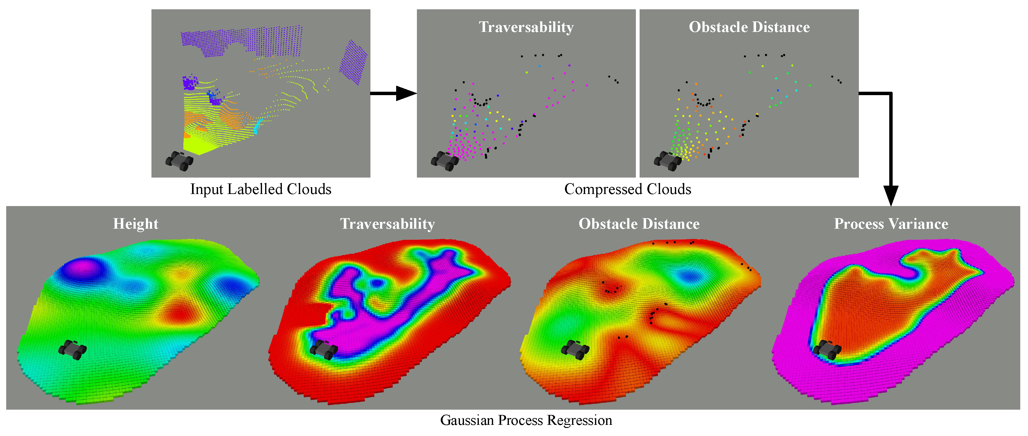
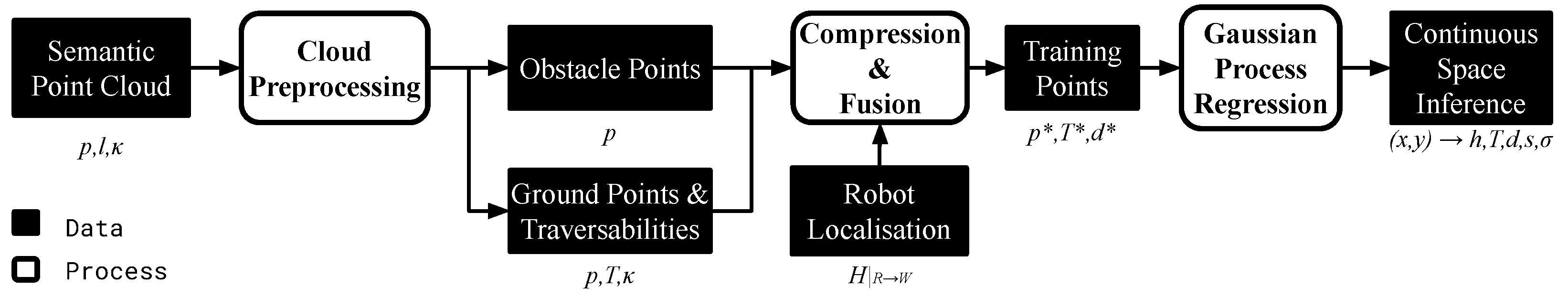
3. GPR Online Implicit Environment Representation

The proposed methodology aims to provide an online differentiable regression of the robot environment from semantic point clouds (see Figure 1 and Figure 2). Inspired by recent literature [9,34], a selection of four variables were deemed relevant for robot navigation: the traversability T associated to the terrain class, the distance d between the robot and obstacles, the terrain height h and its slope s. Online regression is performed with the use of a statistical implicit representation providing variance on inference, after compression of the input clouds. Gaussian processes are employed here but can be replaced by other methods with similar statistical properties. The output of this pipeline is a regression of the T, d and h variables that can be inferred in a continuous 2D space for informative robot navigation. The terrain slope s is calculated by differentiating the height regression. Input clouds are expressed in a frame $R_t$ linked to the robot at the current time t and regression is performed in the fixed world frame W. The GPR method presented in this section can be used for local or small scale environment representations, due to computational constraints. A possible adaptation of this method for global large scale environment representation is given later in Section 6.2.3.

3.1. Input Data and Preprocessing

Camera images and depth maps or LiDAR clouds can be used to produce the required semantic point clouds thanks to the use of a semantic segmentation Convolutional Neural Network (CNN) such as [35,36]. The latter are usually employed to allocate semantic labels to sensor data (typically image pixels or 3D points) after learning such associations by training from data annotated with labels belonging to a pre-defined set. These predictions are commonly associated with a network confidence value. The resulting semantic cloud S is a set of 3D points p of coordinates $(x,y,z)$ with each point associated to a label l belonging to a fixed set L of labels and a classification confidence $\kappa$.

$$p={\left[\begin{array}{ccc}x& y& z\end{array}\right]}^T\in {\mathbb{R}}^3,l\in L,\kappa \in [0,1]$$

(1)

It is assumed that the robot localisation is handled by an external system. A state-of-the-art LiDAR SLAM was used in the experiments. The relative transform between a fixed referential and the robot must be provided at least at the same rate as the semantic clouds. For each received semantic point, T is obtained from its label using a conversion function f based on the robot locomotion modality and the terrain traversability. In our case, a coefficient lookup table, inspired from the analysis presented in [34] is employed. Classes considered as obstacles are associated to a traversability equal to 0.

$$T=f\left(l\right)\in [0,1]$$

(2)

At time t, the cloud points are then separated between ground $G_t$ and obstacles $O_t$ using their traversability values. The first will be used to represent the surface on which the robot will be able to navigate whereas the second will be used to estimate the distance to obstacles from any coordinate on that surface:

$$O_t=\left\{p_i\right\},T_i=0G_t=\left\{p_i\right\},T_i>0$$

(3)

3.2. Point Clouds Compression and Fusion

As GPR inference classically scales in $O\left(n^3\right)$ with the size of its training set, the number of points that can be used for its online training must be limited in order to satisfy the real-time constraints of its targeted applications. A compression and fusion of the information contained in the pre-processed semantic clouds is consequently proposed. In this section, we describe two different algorithms employable for this purpose: a grid clustering (Section 3.2.1) and a two-step k-means clustering (Section 3.2.2). They are evaluated and compared in Section 5.2.

3.2.1. Grid Clustering Compression

Grid clustering is a widely used method for point cloud compression and down-sampling. It presents the advantage of being fairly simple and produces clusters that are uniformly distributed. Moreover, since clusters are associated to cell coordinates, they can be recursively fused over time with newly acquired points. The pre-treated ground cloud $G_t$ and obstacle cloud $O_t$ resulting from the previously described treatment performed at time t are expressed in the current robot frame $R_t$. They are transformed to the world frame using the homogeneous transform matrix ${H|}_{R_t\to W}$ between the two frames.

$$G_t{{|}_W=\{H{|}_{R_t\to W}·p\},p\in G_t|}_{R_t}$$

(4)

$$O_t{{|}_W=\{H{|}_{R_t\to W}·p\},p\in O_t|}_{R_t}$$

A 2D grid of chosen cell resolution r is drawn on the $(x,y)$ plane. All points of $G_t{|}_W$ falling within the boundaries of the same cell c of center $(x_c,y_c)$ are considered as part of the same cluster ${\mu }_{c,t}$.

$${\mu }_{c,t}=\left\{p\right\}\subset G_t{|}_W,\begin{array}{c}x\in [x_c-{\displaystyle \frac{r}{2}},x_c+{\displaystyle \frac{r}{2}}]\\ y\in [y_c-{\displaystyle \frac{r}{2}},y_c+{\displaystyle \frac{r}{2}}]\end{array}$$

(5)

One compressed point $p_{c,t}^{\ast }$ per cell is then computed as the recursive mean of the 3D coordinates of all points of the cell cluster. A traversability value $T_{c,t}^{\ast }$ is computed from the recursive mean of the cluster points traversabilities weighted by their network confidence. $w_{c,t}^p$ denotes the weight of the compressed coordinates stored in the cell and $w_{c,t}^T$ denotes the weight of its traversability value at time t. $|{\mu }_{c,t}|$ denotes the cell cluster cardinality.

$$w_{c,t}^p=w_{c,t-1}^p+\left|{\mu }_{c,t}\right|p_{c,t}^{\ast }={\displaystyle \frac{1}{w_{c,t}^p}}·\left(p_{c,t-1}^{\ast }·w_{c,t-1}^p+\sum _{i=1}^{|{\mu }_c|}{p}_i\in {\mu }_{c,t}\right)$$

(6)

$$w_{c,t}^T=w_{c,t-1}^T+\sum _{i=1}^{|{\mu }_c|}{\kappa }_i{T}_{c,t}^{\ast }={\displaystyle \frac{1}{w_{c,t}^T}}·\left(T_{c,t-1}^{\ast }·w_{c,t-1}^T+\sum _{i=1}^{|{\mu }_c|}{T}_i.{\kappa }_i\right)$$

(7)

A similar processing is applied to the points of the obstacle cloud $O_t{|}_W$: a compressed obstacle point $o_{c,t}^{\ast }$ is computed as the recursive mean of all obstacle points falling within the cell boundaries, as in the following two equations. ${\nu }_{c,t}$ is the cluster of obstacles associated to c and $w_{c,t}^O$ the weight for the cell compressed obstacle coordinates at time t.

$${\nu }_{c,t}=\left\{p\right\}\subset O_t{|}_W,\begin{array}{c}x\in [x_c-{\displaystyle \frac{r}{2}},x_c+{\displaystyle \frac{r}{2}}]\\ y\in [y_c-{\displaystyle \frac{r}{2}},y_c+{\displaystyle \frac{r}{2}}]\end{array}$$

(8)

$$w_{c,t}^O=w_{c,t-1}^O+\left|{\nu }_c\right|o_{c,t}^{\ast }={\displaystyle \frac{1}{w_{c,t}^O}}·\left(o_{c,t-1}^{\ast }·w_{c,t-1}^O+\sum _{i=1}^{|{\nu }_{c,t}|}{p}_i\in {\nu }_{c,t}\right)$$

(9)

The set of compressed ground and obstacle points coordinates resulting from this process are respectively denoted by $G_t^{\ast }$ and $O_t^{\ast }$.

A filtering algorithm is then employed to ensure that the obstacle distance field produced by the GPR includes a confidence measure on occupancy with respect to successive observations. For this purpose, each cell stores an obstacle observation counter that is increased every time an obstacle is observed inside the cell and decreased when no obstacle is observed but a ground point is. If the counter falls to 0, the compressed obstacle is removed. In order to limit the GPR training set maximum size, grid compression is applied locally around the robot, and compressed points and obstacles are discarded once they are further than a fixed distance $d_{max}$ from the robot position.

3.2.2. Two-Steps k-Means Clustering Compression

K-means clustering is another vastly employed method for data compression. As opposed to grid clustering, it allows to preserve the input data distribution after compression. In order to allow fusion between successively produced compressed points while remaining computationally efficient, we propose to use a two-step spatio-temporal compression of the received clouds using k-means clustering. First, a spatial compression is performed on $G_t$ at any given time instant using k-means clustering $\mathcal{K}(.)$ [37] over the 3D points with a parameterised number $k_{\mathcal{S}}$ of clusters ${\mu }_i$ whose cardinality is denoted by $|{\mu }_i|$, as

$$\underset{\phantom{(}i\in \{1,..,k_{\mathcal{S}}\}}{\left\{{\mu }_i\right\}}=\mathcal{K}\left(G_t\right),{\mu }_i=\underset{\phantom{(}j\in \{1,\cdots ,|{\mu }_i\left|\right\}}{\left\{p_j\right\}}$$

(10)

Pseudo-points $p^{\#}$ are then created as the mean 3D coordinates of all points associated to each cluster ${\mu }_i$ and a traversability $T^{\#}$ is computed from the average of the cluster points traversabilities weighted by their network confidence.

$$p_i^{\#}={\displaystyle \frac{1}{|{\mu }_i|}}·\sum _{j=1}^{|{\mu }_i|}{p}_j\in {\mu }_i{T}_i^{\#}={\displaystyle \frac{1}{{\sum }_{j=1}^{|{\mu }_i|}{c}_j}}·\sum _{j=1}^{|{\mu }_i|}{T}_j.{\kappa }_j$$

(11)

The pseudo-point and obstacle clouds generated at instant t are respectively denoted $G_t^{\#}$ and $O_t$. These clouds, expressed in their current robot frame $R_t$, are transformed to the world frame using the homogeneous transform matrix ${H|}_{R_t\to W}$ between the two frames.

$$G_t^{\#}{{|}_W=\{H{|}_{R_t\to W}·p\},p\in G_t^{\#}|}_{R_t}$$

(12)

$$O_t{{|}_W=\{H{|}_{R_t\to W}·p\},p\in O_t|}_{R_t}$$

A second k-means clustering operation $\mathcal{K}(.)$ is performed on the union of the n last pseudo-point clouds with a parameterised number of clusters $k_{\mathcal{T}}$ for temporal compression.

$$\underset{\phantom{(}i\in \{1,..,k_{\mathcal{T}}\}}{\left\{{\mu }_i^{\#}\right\}}=\mathcal{K}\left(\bigcup _{k=t-n}^t{G}_k^{\#}{|}_W\right),{\mu }_i^{\#}=\underset{\phantom{(}j\in \{1,\cdots ,|{\mu }_i^{\#}\left|\right\}}{\left\{p_j^{\prime }\right\}}$$

(13)

The new compressed points coordinates $p^{\ast }$ and traversability values $T^{\ast }$ are computed as the average of the coordinates and traversabilities of pseudo points associated to each cluster ${\mu }_i^{\#}$ weighted by their respective cardinality.

$$p_i^{\ast }={\displaystyle \frac{1}{{\Sigma }_{j=1}^{|{\mu }_i^{\#}|}\left|{\mu }_j\right|}}·\sum _{j=1}^{|{\mu }_i^{\#}|}{p}_j^{\prime }·|{\mu }_j|T_i^{\ast }={\displaystyle \frac{1}{{\Sigma }_{j=1}^{|{\mu }_i^{\#}|}\left|{\mu }_j\right|}}·\sum _{j=1}^{|{\mu }_i^{\#}|}{T}_j^{\prime }·\left|{\mu }_j\right|$$

(14)

The set of compressed point coordinates is denoted by $G_t^{\ast }$. The set of considered obstacle points $O_t^{\ast }$ is the union of the n last received obstacle clouds.

3.2.3. Obstacle Distance Computation

Posterior to the compression process, regardless of the chosen method, the 2D obstacle distances are calculated for all compressed points of $G_t^{\ast }$ with respect to all points of $O_t^{\ast }$ as follows.

$$\forall p_i^{\ast }\in G_t^{\ast }\forall o_j\in O_t^{\ast },d_i^{\ast }=\underset{j}{min}∥p_i^{\ast },o_j∥$$

(15)

The resulting compressed points $p^{\ast }=\left[\begin{array}{ccc}{x}^{\ast }& y^{\ast }& z^{\ast }\end{array}\right]$ associated to their traversabilities $T^{\ast }$ and their distances to obstacles $d^{\ast }$ can then be used to train the GPR.

3.3. Gaussian Process Regression

As the goal of this process is to provide an implicit representation of the ground surface height, traversability and distance to obstacles, the compressed points produced by each of the previously described processes can be used as training points for the calculation of a GPR [38] of these variables over a 2D horizontal plane. A correlation matrix $K(X,X)$ is computed on the set X of compressed 2D point coordinates $X_i=[x_i^{\ast },y_j^{\ast }]$ where each element of the matrix stores the correlation between two points $X_i$ and $X_j$ defined by the correlation kernel $\mathit{k}$ such that ${K(X,X)|}_{i,j}=\mathit{k}(X_i,X_j)$. The correlation vector $K(q,X)$ between any 2D query point q and the training points is calculated as ${K(q,X)|}_i=\mathit{k}(q,X_i)$. The latter are used to infer the values of T, d and h at the query point coordinates as shown in Equation (16), where ${\mathit{T}}^{\ast }$, ${\mathit{z}}^{\ast }$ and ${\mathit{d}}^{\ast }$ respectively denote the vectors of all training outputs $T^{\ast }$, $z^{\ast }$ and $d^{\ast }$ corresponding to the training points in X.

$$\begin{array}{c}\hfill \widehat{T}\left(q\right)=K{(q,X)}^T·{[K(X,X)+o_n^2·I]}^{-1}·{\mathit{T}}^{\ast }\\ \hfill \widehat{h}\left(q\right)=K{(q,X)}^T·{[K(X,X)+o_n^2·I]}^{-1}·{\mathit{z}}^{\ast }\\ \hfill \widehat{d}\left(q\right)=K{(q,X)}^T·{[K(X,X)+o_n^2·I]}^{-1}·{\mathit{d}}^{\ast }\end{array}$$

(16)

The observation noise variance $o_n^2$ is an hyperparameter of the process (see Section 4.1). The terrain slope norm regression $\widehat{s}$ can be easily computed at any query coordinates thanks to the availability of the differentiable closed form expression of the GPR as follows:

$$\widehat{s}\left(q\right)=\sqrt{{\left({\displaystyle \frac{\partial \widehat{h}}{\partial x}}\right)}^2+{\left({\displaystyle \frac{\partial \widehat{h}}{\partial y}}\right)}^2}$$

(17)

Finally, the process variance at coordinates contained in q is given as follows:

$${\widehat{\sigma }}^2\left(q\right)=K(q,q)-K{(q,X)}^T·{[K(X,X)+o_n^2·I]}^{-1}·K(q,X)$$

(18)

This inference process can be used on the fly for short horizon planning or stored in a global structure for large-scale environments. The flexibility induced by this continuous representation allows various kind of planning algorithms to be used and the availability of a process variance can be taken in account to improve safety when planning or as a knowledge metric for exploration purposes.

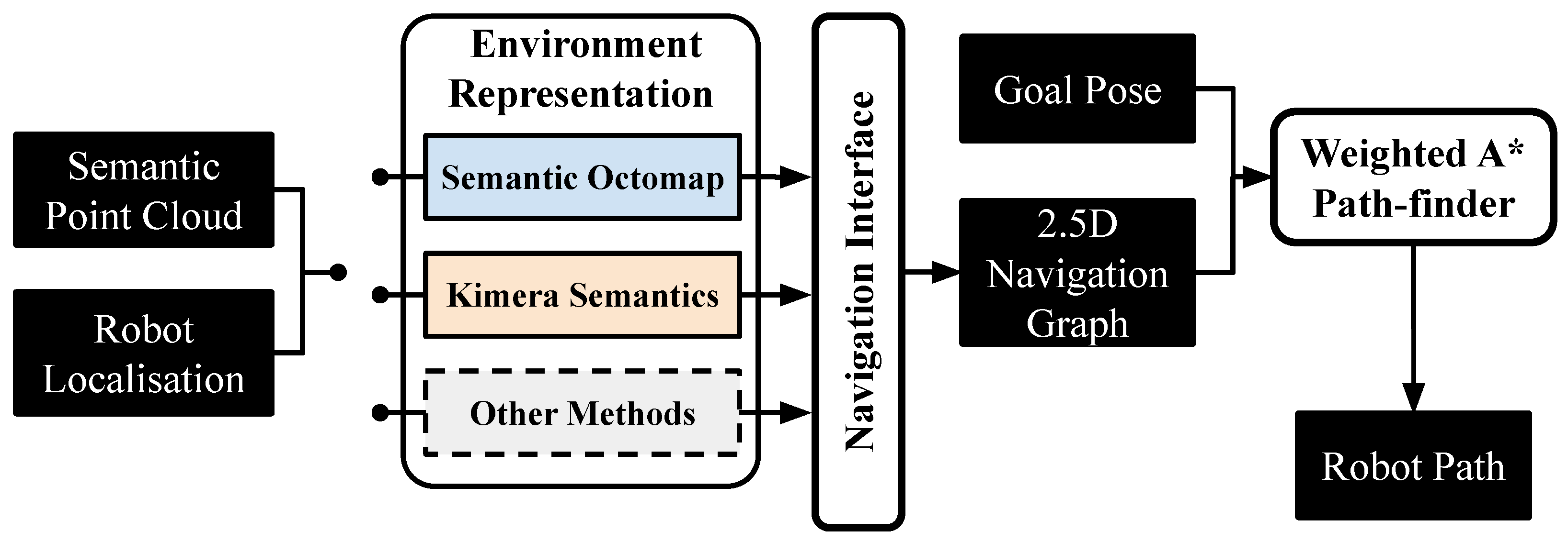
4. The COSMAu-Nav Architecture

This section introduces the Continuous Online iMplicit representation for Autonomous Navigation COSMAu-Nav architecture that relies on the above-described GPR environment representation to perform online path-planning both at a fine level on a local scale and at a coarse level on a global scale. The COSMAu-Nav architecture has been developed using ROS, it is intended to be publicly released. The architecture is illustrated in Figure 3. It comprises a cloud preprocessing step, filtering ground and obstacles and allocating traversability values to semantic labels, followed by one of the cloud compression methods presented in Section 3.2. The produced compressed points are then given as training inputs to a local GPR, used by a local planner to produce coarse priors and smooth paths for the robot to follow. The outputs of the compression process can be used by an auxiliary global environment representation and navigation module to produce local navigation goals. The latter will not be addressed in this section but such an applicative use-case is described in Section 6.2.3.

4.1. Implementation of the GPR Environment Representation Method

The following section describes the implementation choices that allowed the GPR environment representation method to run online on a computer equipped with a desktop GPU that can be mounted on a ground robot.

Grid clustering compression: The grid clustering has been efficiently implemented thanks to the binned statistics functionality of the SciPy library [39].

K-means clustering compression: The spatial k-means clustering is implemented in a mini-batch form [37]. This form of k-means clustering introduces stochasticity in the process but allows fast and economical convergence. While the size of the clouds resulting from this first compression can be controlled to be limited and allow the second k-means temporal clustering to be exhaustive, it has been decided to implement the latter with GPU acceleration as this step could represent one of the limitations for high-rate processing.

GPR training and inference: GPR was implemented using GPyTorch [40], a PyTorch based GPU-accelerated Gaussian process regression library. Fast GPR inference for large batches of query points is allowed thanks to the exploitation of the LOVE posterior covariance estimation [41] implemented in GPyTorch. Note that a GPJax (JAX based library for Gaussian process applications) implementation has been tested as well but turned out to be less efficient as JAX strength lies in its ability to pre-compile operations on fixed sized data, which is not always the case with our GPR training set. A Radial Basis Function (RBF) has been chosen as correlation kernel $\mathit{k}$ where the length-scale $L_k$ and the variance ${\sigma }_k^2$ are the kernel hyperparameters.

$$\mathit{k}(X_i,X_j)=L_k·exp-{\displaystyle \frac{\left(\right|x_i-x_j|+|y_i-y_j{\left|\right)}^2}{2{\sigma }_k^2}}$$

(19)

This kernel is well suited to model smoothly changing environments such as natural hills and presents the advantage of having a small number of hyperparameters. Any other correlation kernel can be used depending on the context of application and the available computational capacity. The hyperparameters ${\sigma }_k^2$, $L_k$ and $o_n^2$ are trained with GPyTorch on initialisation using the GP marginal log-likelihood as loss function and the ADAM optimiser, after receiving the first compressed cloud.

4.2. Smooth Path Planning in the GPR Environment Representation

The robot safety and its locomotion efficiency being a primary concern in the context of a navigation task in an outdoor environment, great care must be taken into designing a path-planning algorithm that employs the environment representation at best to satisfy these requirements. As the GPR environment representation presented in Section 3.3 exhibits continuous and differentiable properties, the latter can be put to use by employing gradient-based optimisation for smooth path planning. The exploitation of such environment representations to perform smooth path planning has been introduced in [42] and is summarized in the following for completness. The planned paths are represented as 2D Bézier curves, which are flexible parametric functions defined for $t\in [0,1]$ by a set of control points $P=\left\{P_i\right\},i\in [0,\cdots ,n-1]$ with $P_i=(x_i,y_i)$ as follows:

$$B(t,P)=\sum _{i=0}^{n-1}{\displaystyle \frac{n!}{i!(n-i)!}}{t}^i{(1-t)}^{n-i}{P}_i$$

(20)

The position of these control points can be optimised to satisfy certain requirements on the robot motion by searching for the minimum of a differentiable loss function:

$$\underset{P\in {\mathbb{R}}^{2n}}{min}L\left(B(t,P)\right)$$

(21)

This loss function consists in a sum of differentiable criteria on each aspect of the terrain and robot locomotion deemed significant for its navigation, each term weighted by a given coefficient.

$$L\left(B(t,P)\right)=f_l.L_l+f_T.L_T+f_{\sigma }.L_{\sigma }+f_o.L_o+f_c.L_c$$

(22)

With:

• $L_l$ and $f_l$ the loss term and coefficient relating to the path length
• $L_T$ and $f_T$ the loss term and coefficient relating to terrain traversability
• $L_{\sigma }$ and $f_{\sigma }$ the loss term and coefficient relating to the process variance
• $L_o$ and $f_o$ the loss term and coefficient relating to obstacle collision
• $L_c$ and $f_c$ the loss term and coefficient relating to the path curvature

These terms are explicited in the dedicated article [42] and are kept unchanged in this application, at the exception of the traversability loss term $L_T$ that has been adapted to take the terrain slope into account as follows:

$$L_T={\int }_0^1(1-\widehat{T}(x,y))(1+\widehat{s}(x,y))dt$$

(23)

To prevent the optimisation to fall in unpractical local minima and to speed up the optimisation process, the initial position of the Bézier curve control points is given by a prior sampling-based planner using the T-RRT algorithm as described in [1]. This complete operation allows to generate paths that satisfy requirements in terms of robot safety, compliance to the robot kinematics and locomotion capacities with respect to the terrain properties, as demonstrated in the simulated experiments pursued in [42].

5. Experimental Evaluations

As a mean to evaluate the quality of the environment representation produced by the COSMAu-Nav architecture, experiments have first been carried out in a simulated Gazebo environment. The objectives and metrics of these evaluations are presented in Section 5.1. Aiming to select the most suitable compression method for embedded online usage in COSMAu-Nav, Section 5.2 presents a comparative study between the compression algorithms described in Section 3.2. Subsequently, the robustness of the environment representation quality produced by COSMAu-Nav to localisation noise and semantic segmentation errors has been measured and compared against the previously developed SMaNA architecture, briefly described in Section 5.3. The results of these evaluations are displayed and discussed in Section 5.4. Both architectures have been applied to produce environment representations with real-world sensor data from the Rellis-3D dataset, their computational performances and memory workloads have been compared in Section 5.5.

5.1. Gazebo Simulation Evaluation Setup

A Gazebo 3D simulation has been built for the evaluation and comparison of the methods (more details in [2]). It consists of a 12 m × 12 m environment built from the 3DRMS synthetic outdoor navigation dataset [3]. It includes a wheeled differential-drive UGV (Wifibot) model with a footprint radius of 0.125 m and a height of 0.25 m equipped with a camera module producing depth maps and semantic images of resolution $200\times 200$ at a 10 Hz rate. Points further than 3 m from the robot are cut out. The latter are used to produce a 3D semantic cloud thanks to a geometric projection module. The ground truth robot pose is available. The simulated robot has been set to follow a 50 m path at a speed of 0.4 m/s inside this environment. The ground surface of the simulated environment is composed of two different terrain classes: dirt and grass, their respective traversabilities have been set to 1.0 and 0.25. The different elements of this simulation are illustrated in Figure 4 and the association between semantic classes labels, colors and traversabilities are presented in

Table 2. Colors and traversabilities associated to semantic classes contained in the simulation.

class	sky	grass	terrain	hedge	topiary	rose	obstacle	tree
color
traversability	0	0.2	1	0	0	0	0	0

. The environment mesh has been used to produce ground-truth navigation grids at multiple resolutions from 0.1 m to 0.25 m whose cells store a height value, a traversability value and an obstacle occupancy. In order to build these reference grids, the 3D mesh is first converted to a labelled point cloud of uniform high density, traversability values are then calculated for each point belonging to the ground. Each cell of the grid is granted a height value corresponding to the average height of the ground points within its 2D borders. The distance to the closest obstacle is calculated from each cell centre and the nodes with obstacle distances smaller than the safety threshold are marked as occupied. The traversability of each cell is calculated as the average traversability of all points within the robot footprint around the cell centre. This choice allows to take the robot footprint into account and conveys a preference to travel in the middle of a path rather than on the side of it, thus penalising the edges of high traversability zones bordering lower traversability zones. These reference grids are used to evaluate the quality of each presented method environment representation with four different metrics.

The occupancy classification accuracy $\mathit{OA}$ was calculated with ${\mathit{TP}}_o$, ${\mathit{FP}}_o$, ${\mathit{TN}}_o$, ${\mathit{FN}}_o$ respectively being the true and false positive and negative for obstacle occupancy classification in the reference grids.

$$\mathit{OA}={\displaystyle \frac{{\mathit{TP}}_o+{\mathit{TN}}_o}{{\mathit{TP}}_o+{\mathit{FP}}_o+{\mathit{TN}}_o+{\mathit{FN}}_o}}$$

(24)

For each following evaluation, the traversability and height cell-wise errors $ϵ\left(h\right)$ and $ϵ\left(T\right)$ have been computed for cells existing in the reference grids and considered observed by the environment representation methods. The error distributions are represented as box plots, with the center line of each box representing the mean, the edges the first and third quartiles and the whiskers the 95% confidence interval of their Gaussian fit. The map discovery recall ($\mathit{DR}$) is computed for each evaluated method as the ratio of cells existing in the reference grid and considered observed by the environment representation methods over the total number of cells in the reference grid.

For every evaluation, the CPU and GPU consumption as well as the RAM usage have been recorded. The average update rate of the environment representation has been measured. The dispersion of these variables being very low for all performed experiments, only their average value is displayed. All experiments were performed on an Intel Xeon(R) W-2123 8 core 3.60 GHz CPU with 16 GB of RAM and a NVIDIA GeForce GTX 1080 GPU with 8 GB of RAM.

5.2. Comparison of Point Cloud Compression Methods

In order to identify the most suitable point cloud compression method for embedded usage in the COSMAu-Nav architecture and to understand the influence of their parameters, an ablation study has been performed on the two methods presented in Section 3.2. Both have been evaluated in terms of mapping quality and computational load in the above-described simulated context. They have been employed to process the data gathered by the simulated robot sensors along its trajectory for the GPR to produce a representation of the observed environment, compare it to the reference navigation grids and measure its computational performances. Compressed points produced by each method are kept in memory for the duration of the entire trajectory. Local GPR inference is performed at compressed points production rate for visualisation on a grid of selected resolution $ir$ in the convex envelop of the compressed points within a 3 m radius from the robot position. When reaching the end of the trajectory, inference is performed once in the entire environment boundaries with all produced compressed points as training data. The nominal parameters of each compression method and of the GPR environment representation are given in

Table 3. Summary of the compression methods and GPR nominal parameters for their application in simulation.

Parameter	Value
Grid Clustering Compression
Point integration max distance	3.0 m
Resolution of the clustering grid	0.25 m
Distance from the robot beyond which a cluster is discarded	15 m
K-means Clustering Compression
Number of clusters for k-means spatial compression	100
Number of clusters for k-means temporal compression	200
Number of scans in the temporal integration window	10
GPR
Safety radius: threshold distance from obstacles below which a point is considered as occupied	0.25 m
Inference resolution for online visualisation	0.1 m
Threshold process variance above which the space is considered unobserved	2.5 × 10−3
Distance from the robot up to which inference is performed for visualisation	3.0 m

. The parameters are fixed to these values when the influence of the others is evaluated as follows:

• The grid resolution for grid clustering compression r at 0.2 m, 0.25 m, 0.3 m, 0.35 m and 0.4 m.
• The number of clusters for the k-means spatial compression step $k_{\mathcal{S}}$ at 50, 100, 150, 200 and 250.
• The number of clusters for the k-means temporal compression step $k_{\mathcal{T}}$ at 50, 100, 150 and 200.
• The GPR inference resolution $ir$ at 0.0 m (no local inference), 0.05 m, 0.1 m, 0.15 m, 0.2 m and 0.25 m.

Ten runs have been conducted for each evaluation with the k-means clustering, as it includes statistical treatments.

As the main objective of this study is to obtain the best ratio between the produced environment representation quality and its computational requirements, a summary of its results is presented in Figure 5 which displays the average obstacle accuracy ($OA$), absolute average terrain traversability error ($ϵ\left(T\right)$) and absolute average terrain height error ($ϵ\left(h\right)$) in function of the average induced CPU and GPU loads for all the evaluated parameter values. Figure A1 displays the detailed influence of grid clustering resolution and k-means number of clusters for spatial and temporal compression over all representation quality and computational performance metrics.

The presented result show a clear superiority of the grid clustering method in terms of computational performances, requiring less CPU and GPU processing power than k-means clustering for every evaluated parameter value, with an average reduction of the CPU load of 36% and of GPU load of 50%. It allows to process point clouds at their production rate of 10 Hz against a best processing rate of 4.4 Hz for k-means clustering. It also requires 43% less RAM capacity in average. Moreover, over all evaluations, the obstacle accuracy of the GPR environment representation produced with grid clustering compression are higher (10% improvement in average) and their terrain traversability error lower than with k-means clustering compression. K-means clustering seems however to provide a slight improvement in terms of terrain height error.

The influence of the process variance threshold $t_{{\sigma }^2}$ on the environment representation accuracy produced by both methods is displayed in Figure 6. The process variance threshold evaluation clearly indicates that the higher we set the threshold, the more space we can consider as observed at the cost of representation accuracy. Its value must thus be selected accordingly to a trade-off between exhaustiveness and accuracy of the representation.

The results and conclusions drawn from this evaluation led us to choose grid clustering over k-means clustering for point cloud compression in COSMAu-Nav following applications, as its implementation appears more computationally efficient while improving the environment representation quality.

5.3. Baseline Discrete Semantic Mapping and Navigation Architecture (SMaNA)

For evaluation and comparison purposes, the previously developed general-purpose Semantic Mapping and Navigation Architecture (SMaNA) [2], which features a generic navigation grid interface has been used as reference. Two reference discrete explicit semantic mapping methods, described in Section 5.3.1 below have been implemented in the architecture. It employs a weighted A* path-planner as a simple and commonly used method for semantic-aware navigation [23,43,44]. The SMaNA ROS architecture can use a variety of methods for semantic mapping to build a 2.5D 8-connected navigation graph. The latter consists of a 2D grid with parameterised resolution where each node contains an occupancy counter $o\left(n\right)$, a height value $h\left(n\right)$ and a traversability value $T\left(n\right)$. The interface between the mapping methods and the graph building is specific to each method, but the graph data structure and usage are unified for all methods (Figure 7).

An informative A* path-planning algorithm is applied, with a cost of transition from a parent node p to a node n of its neighbourhood consisting of a weighted sum of the distance between their centres, its traversability $T\left(n\right)$ weighted by a factor $T_f$ and the slope $s(n,p)$ between them, weighted by a factor $S_f$.

$$c(p\to n)=\left|[p,n]\right|+T_f·T\left(n\right)+S_f·s(n,p)$$

(25)

The slope between 2 neighbouring nodes $s(n1,n2)$ can be calculated using numerical differentiation of their height over the distance between them.

$$s(n1,n2)={\displaystyle \frac{\left|h\right(n2)-h(n1\left)\right|}{\left|\right[n1,n2\left]\right|}}$$

(26)

The total node cost $c\left(n\right)$ considered by the A* planner is defined as the sum of the transition cost from its parent, its parent total cost and its distance to the goal node g.

$$c\left(n\right)=c\left(p\right)+\left|\right[g,n\left]\right|+c(p\to n)$$

(27)

5.3.1. Discrete 3D Semantic Mapping Methods

The application of COSMAu-Nav has been compared with semantic Octomap [6] and Kimera Semantics [7] in the SMaNA framework.

Semantic Octomap [6]: This method builds an explicit 3D volumic map by allocating occupancy and labels to voxels using max fusion of multiple observations. Voxels are stored in an octree structure for faster access and lighter storage. The updated voxels are incorporated by the SMaNA graph building process and projected in 2D. For each graph node, the voxel of greatest height value under a fixed threshold $t_h$ is selected among the set of voxels of centre coordinates within the node borders. Its height value $h_i$ and traversability $T_i$ associated to its label are allocated to the corresponding node n of the graph. The following equation describes this process, with r being the graph resolution.

$$\begin{array}{c}T\left(n\right)=T_i\\ h\left(n\right)=h_i\end{array},h_i=\underset{j}{max}(h_j<t_h),\begin{array}{c}{x}_j\in [x\left(n\right)-{\displaystyle \frac{r}{2}},x\left(n\right)+{\displaystyle \frac{r}{2}}]\\ y_j\in [y\left(n\right)-{\displaystyle \frac{r}{2}},y\left(n\right)+{\displaystyle \frac{r}{2}}]\end{array}$$

(28)

Since obstacle distance is not directly available in the Octomap representation, it is handled in the navigation graph. Each node contains an obstacle counter, which is incremented if an occupied voxel is closer than a safety distance threshold. This counter is decremented if surrounding nodes are later estimated as traversible.

Kimera Semantics [7]: This method based on [45] applies the TSDF methodology [46] to populate a 3D voxel grid with signed distances to surfaces using ray-casting and associate semantic labels to voxels along the rays using Bayesian fusion of observations. A marching cubes algorithm is used to produce a semantic 3D surfacic mesh representing the robot environment. The semantic TSDF voxels are stored in blocks that are hashed for lighter storage and faster transfer. These blocks are deserialised and the retrieved TSDF voxels of absolute distance values smaller than the mapping resolution are integrated into the navigation graph in the exact same fashion as Octomap voxels.

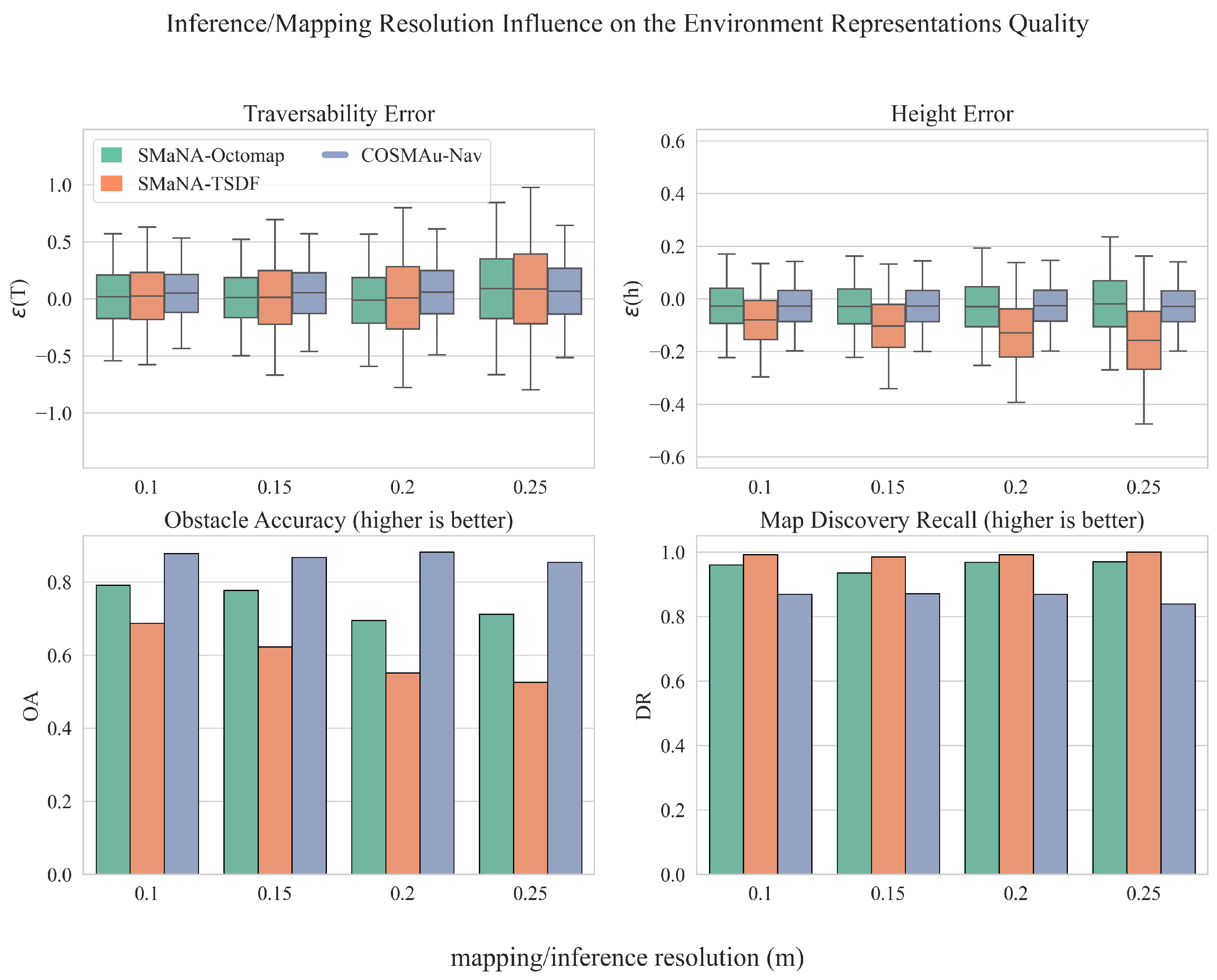
5.4. Comparison of the GPR Environment Representation with the SMaNA Baseline

The influence of mapping and inference resolution on the previously described metrics has been evaluated for four different resolution values (10 cm, 15 cm, 20 cm and 25 cm).

Synthetic degradation of input localisation is applied by adding a zero-mean Gaussian noise of parameterised standard deviation to the robot position and yaw angle. Three values for the standard deviations of localisation and yaw angle noise have been selected for this evaluation: (5 cm, 0.05 rad), (10 cm, 0.1 rad) and (20 cm, 0.2 rad).

To carry out a controlled evaluation of the influence of classification errors, semantic segmentation ground truth images have been artificially degraded. They were segmented in super-pixels [47] and each super-pixel has been assigned a probability to be misclassified according to a confusion matrix between semantic classes, inspired by the confusion of a CNN in real-life settings. Three segmentation misclassification probabilities have been selected for this evaluation: 0.05, 0.25 and 0.45.

The main nominal parameters of the methods described in Section 5.3 are presented in

Table 4. Summary of the main nominal parameters of Semantic Octomap, Kimera Semantics and the SMaNA navigation graph builder for their application in simulation.

Parameter	Value
Semantic Octomap
Maximum point integration range	3.0 m
Resolution of the octree leaf voxels	0.1 m
Ray casting range	3.0 m
Occupancy threshold	0.5
Kimera Semantics
Maximum point integration range	3.0 m
Voxel size	0.1 m
Voxels per bloc side	16
Voxel update method	“fast”
Navigation Graph Building
Safety radius: threshold distance from obstacles below which a cell is considered as occupied	0.25 m
Navigation graph grid cell resolution	0.1 m

. The nominal parameters used for COSMAu-Nav grid clustering compression and GPR are the same as presented in Table 3.

A visualisation of the environment representation for robot navigation produced by the compared methods with nominal parameters and of the trajectory followed by the robot in the simulated environment is given in Figure 8. The GPR environment representation has been inferred on an uniform 2D grid of same resolution as the other evaluated methods to produce the displayed visualisation.

Figure 9 displays the influence of the inference and mapping resolution over the representation quality metrics for the three evaluated methods. No degradation was applied to input data for this experiment. The GPR representation outputs an absolute improvement over all accuracy metrics ($OA$, $ϵ\left(T\right)$, $ϵ\left(h\right)$). Its discovery recall is however lower, this is due to the restrictive threshold set on process variance that can be tuned to consider more space as observed at the cost of accuracy (see Figure 6). These results also highlight the fact that the GPR inference resolution has a much less significant impact on the generated map accuracy than for both other methods. For example, the absolute mean traversability error is increased by 40% between inference resolutions of 10 and 25 cm against 250% and 400% for TSDF and Octomap and its standard deviation is increased by 19% against 47% and 36% respectively.

Figure 10 displays the influence of the robot localisation noise over the representation quality metrics for the three evaluated methods. These results demonstrate the robustness of the GPR environment representation to localisation noise, with a drop of the obstacle accuracy of 12% between its lowest and highest levels against 34% and 35% for TSDF and Octomap. The influence of localisation noise over traversability accuracy is similar for all methods with an increase of the absolute error bias of 94%, 95% and 104% for the GPR, TSDF and Octomap. GPR height regression seems more robust to such degradation with an 8% error mean and 30% standard deviation increase against 75% and 39% for TSDF and 265% and 101% for Octomap. The robot localisation noise seems to have a low impact on the discovery rate of the GPR and Kimera Semantics and affects Semantic Octomap discovery rate only at its highest level.

Figure 11 displays the influence of the semantic segmentation degradation over the obstacle accuracy and traversability error for the three evaluated methods. The discovery rate and height error metrics have been discarded for this evaluation since the impact of semantic segmentation over these metrics is considered of few meaning and influence. Similarly to the previous evaluation, the GPR environment representation appears to be more robust to semantic segmentation error than both other methods with changes in obstacle accuracy and absolute traversability error mean and standard deviation of respectively 2%, 67% and 56% between the lowest and highest semantic segmentation degradation levels against 25%, 870% and 86% for Semantic Octomap and of 7%, 923% and 59% for Kimera Semantics.

The evaluations results displayed in this section show the interest of the Gaussian process regression (GPR) provided by COSMAu-Nav against the Semantic Octomap (Octomap) and Kimera Semantics (TSDF) regarding multiple aspects. Indeed, most evaluated metrics show an absolute performance improvement when using the GPR instead of the other two methods. Indeed, over all evaluation settings, the GPR shows an average terrain traversability accuracy and precision improvement of 15% and 17% against the Octomap and of 35% and 22% against the TSDF. It displays an average terrain height accuracy and precision improvement of 35% and 29% against the Octomap and of 77% and 32% against the TSDF as well as an average obstacle accuracy improvement of 27% against the Octomap and 40% against the TSDF. Furthermore, COSMAu-Nav appears simultaneously more robust to robot localisation noise and semantic segmentation degradation than both Octomap and TSDF, with a significantly lesser impact of the latter on the environment representation metrics.

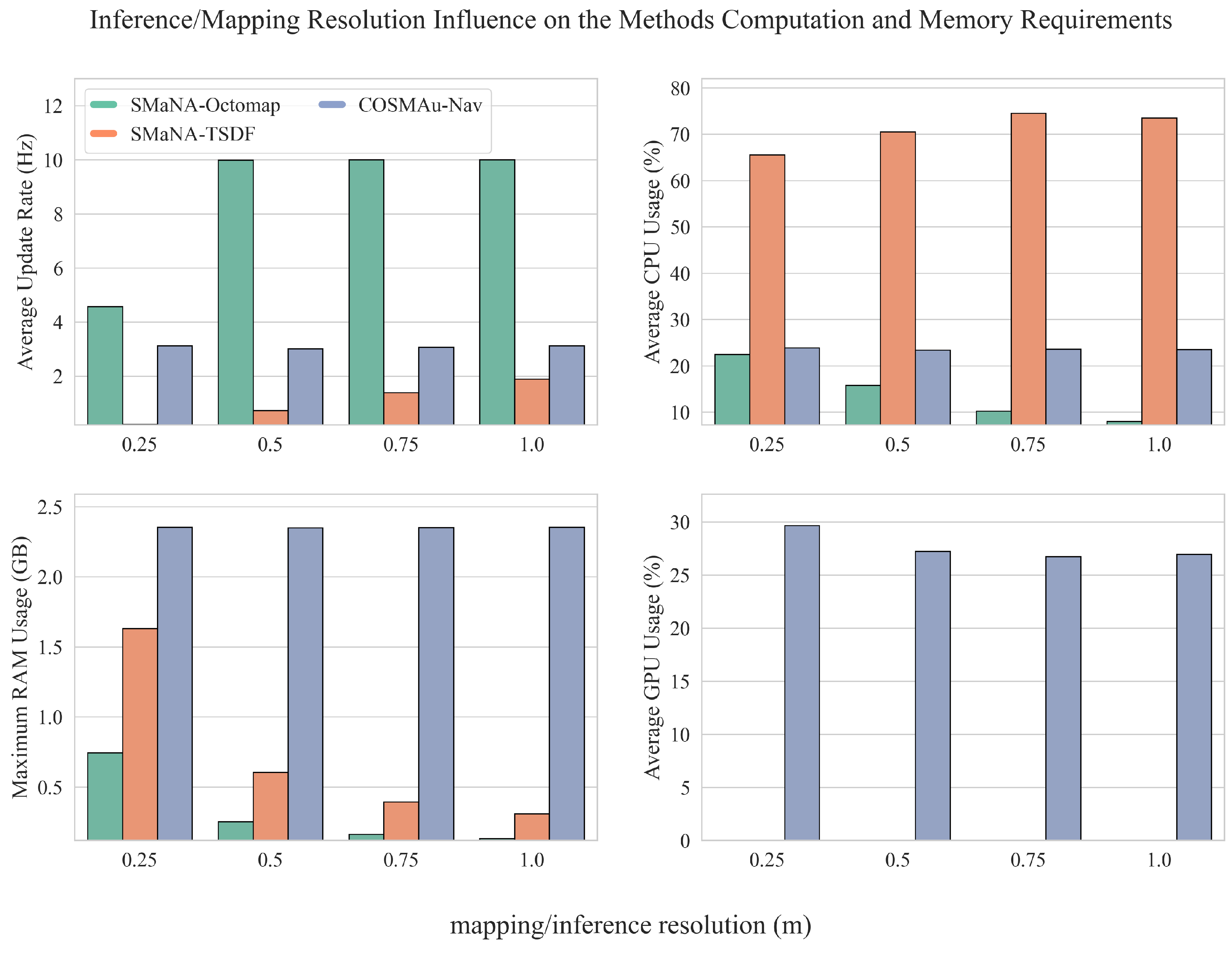
5.5. Analysis of Computational Performances on the Rellis-3D Real-World Dataset

The computational performances of COSMAu-Nav GPR environment representation with grid clustering compression as well as the integration of Semantic Octomap and Kimera Semantics in SMaNA have been measured on the real-world Rellis-3D outdoor UGV dataset [4]. Each has been used to process in real time the sequence 00 of the Rellis-3D dataset. The latter consists of robot poses associated with 3D point-clouds produced at 10 Hz by a LiDAR mounted on a mobile ground robot along a 176 s long trajectory and annotated in post-process. The max point integration distance has been fixed to 12 m and the robot safety radius (R) to 1.0 m for all three methods. the Semantic Octomap ray-casting range has been set to 5 m. COSMAu-Nav grid clustering resolution (r) has been set to 0.5 m, its cluster discard distance ($d_{max}$) and its inference distance for visualisation to 12.0 m. All other parameters remain unchanged from the previous evaluation.

Figure 12 presents the comparative results of this evaluation: the environment representation update rate, total RAM consumption and CPU usage for all methods, and GPU usage for GPR. This evaluation shows that COSMAu-Nav is in fact more expensive to run in terms of memory consumption than both other methods but requires less CPU load than Kimera. It produces updates of the environment representation at a lower rate than the Octomap but higher than Kimera and is still suitable for online usage. In overall, the RAM, CPU and GPU load measured during these evaluations remain in a manageable scope for the employed computer and allow COSMAu-Nav to be used alongside other processes that can be needed in a robot navigation mission such as SLAM or semantic segmentation.

6. Application to a Real-World Autonomous Navigation Mission

The experiments in simulation and on dataset suggested that the proposed architecture achieve a better trade-off between accuracy and computational load than discrete methods for uncertainty-aware navigation in a simulated setting. COSMAu-Nav is able to function online with a desktop computer CPU and GPU and the BCO planning methodology has shown to produce paths of high value for ground robot navigation. Therefore, real embedded tests have been conducted onboard a mobile ground robot for autonomous and safe navigation in a natural, unstructured environment.

6.1. Embedding COSMAu-Nav Onboard a Ground Robot

This section describes the development of a sensor data processing pipeline for the application of COSMAu-Nav on a ground robot for a real-world navigation mission in a natural environment. A representation of this pipeline is given in Figure 13.

For these experiments, a Robotnik Summit-XL differential drive field robot has been employed. It was equipped with an Intel i5-10500 6 core 3.10 GHz CPU with 16 GB of RAM and an NVIDIA GeForce GTX 1650 GPU with 4 GB of RAM. In terms of sensors, an OS0-128 3D LiDAR and a Luxonis OAK-D camera were mounted on the robot. The ROS middleware was used to enable communication between the robot hardware and algorithmic components and between the robot and a remote operator.

Semantic segmentation is performed by the BiseNetV2 CNN [35], which is able to process the camera images at a rate of 5 Hz on the robot embedded GPU. It should exhibit a good level of segmentation in the target context, i.e., an unstructured outdoor environment, for which few datasets or simulated environments are available yet. It has thus been trained with both the Rellis-3D [4] and the RUGD [48] datasets, containing annotated images gathered onboard a ground robot travelling in natural forest and field environments. Geometrical projection of the semantic segmentation image produced by BiseNetV2 onto the 3D LiDAR points is performed so as to obtain the required annotated point clouds. The camera geometric model was provided but can be estimated using calibration methods such as [49]. The precise relative transform between the two sensors has been obtained through the application of the LiDAR-camera calibration tool presented in [50].

The remainder of the architecture is based on the combination of state-of-the-art methods. The open-source implementation of the HDL Graph SLAM method [51] was selected for localisation; it relies on the Normal Distribution Transform (NDT) [52] for LiDAR scan matching. It must be noted that the map built by the SLAM is only used for localisation and that the GPR environment representation is only used for path-planning. Additionally, since the semantic segmentation provided by the CNN is prone to errors, a geometric ground filtering process is applied on the point clouds posterior to the semantic segmentation projection. It is based on an implementation of the CSF ground filtering method [53] and allows the detection of obstacles in the 3D clouds geometry. For safety concerns, it has been decided to rely on both the semantic segmentation and the CSF filtering for obstacle detection. The latter are defined as the union of the obstacle classes identified by the CNN and the obstacles identified by the CSF filtering. The complete pipeline, from sensor data acquisition to path planning, has been integrated and tested on the robot. Illustrations of the data produced by the components described in this paragraph are given in Figure 14.

6.2. Adapting GPR Representation for Multi-Scale Navigation

While GPR in itself can be used for online inference on a controlled number of training points, it is known to scale badly with large training sets. In order to be able to perform global path-planning in large scale environments, a system of keyframe storage and fusion of multiple local GPR inferences has been designed.

6.2.1. Keyframe Storage

The grid clustering compression method presented in Section 3.2, coupled with the GPR inference as described in Section 3.3 allow to obtain online a sliding local regression of the terrain topography, traversability, slope and obstacle distance field. It has been decided to store the points produced by the compression process in a keyframe map, with each keyframe being a collection of compressed ground points associated to the robot pose at the time of the keyframe recording. A distance criterion $d_{kf}$ from the last produced keyframe has been set for the grid clustering method to store the current compressed points as a new keyframe. To prevent information loss and redundancy, it has been fixed to the same value as the compressed point discard range $d_{max}$. Each keyframe pose is associated to the closest graph SLAM keypose, while this feature is not demonstrated here, it allows to propagate the graph SLAM corrections produced by loop-closure detection and pose graph optimisation to the global GPR map.

6.2.2. Global GPR Inference

As explained above, in order to guarantee a controlled computational load and time, GPR regression must be performed on a reasonable number of points at once. Thus, in order to perform inference on a global scale from the keyframe map, a fusion of local GPR inferences is applied. When performing inference in the global map, each 2D query point $q_g$ is associated to a fixed number $n_k$ of its closest stored keyframes and each value ${\widehat{v}}_g$ of the navigation related variables in the global map at those coordinates is estimated as the mean of the inference of the local GPR ${\widehat{v}}_i\left(q_g\right)$ computed with each of these keyframes, weighted by the inverse their process variances ${\widehat{\sigma }}_i^2\left(q_g\right)$. The global process variance at $q_g$ is computed as follows.

$${\widehat{v}}_g\left(q_g\right)={\displaystyle \frac{1}{{\sum }_{i=0}^{n_k}1/{\widehat{\sigma }}_i^2\left(q_g\right)}}\sum _{i=0}^{n_k}{\widehat{v}}_i\left(q_g\right)/{\widehat{\sigma }}_i^2\left(q_g\right)$$

(29)

$${\widehat{\sigma }}_g^2\left(q_g\right)={\displaystyle \frac{1}{{\sum }_{i=0}^{n_k}1/{\widehat{\sigma }}_i^2\left(q_g\right)}}$$

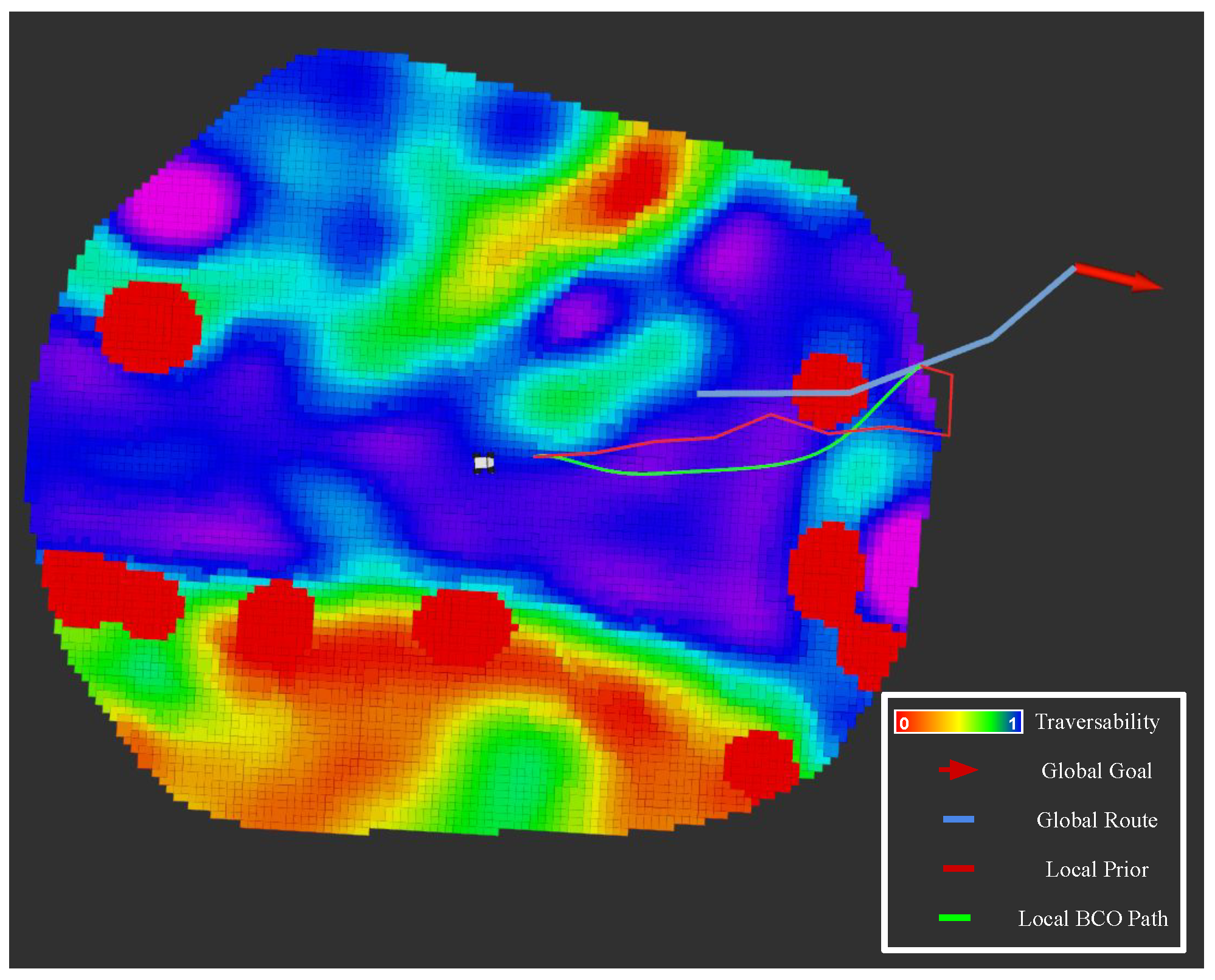
6.2.3. Navigation in the Global Environment Representation

While the method presented in Section 4.2 allows for smooth path-planning with respect to the environment properties, it requires dense queries of the GPR over multiple steps of the planner optimisation. Moreover, when planning long-horizon paths in the global environment, such a level of planning granularity can be superfluous. Therefore, we propose to couple the local proposed planner with a coarse sampling-based global route planning. As the prior planner presented in Section 4.2, it is based on the application of the T-RRT sampling planning methods, its functioning and properties are similar to the latter, with the few following adaptations. First of all, its queries of the environment representation are performed at a global scale, as described in the previous section. The global process variance threshold $t_{{\sigma }^2}$ is employed to allow paths to be planned in the unobserved space. When queries performed in the global map output a process variance superior to this given threshold, the T-RRT transition cost only depends on the distance between their coordinates and the global navigation goal.

6.3. Experiments and Results

The objective of this navigation mission was to demonstrate that the robot is able to reach successive arbitrary way-points given by a remote operator in a previously unknown outdoor environment. A ground-truth point-cloud map of the experiment environment was built by carrying a LiDAR to gather point-clouds, assembled offline with scan-matching and pose graph optimisation available in [51]. This map was used to draw safeguards for the robot to limit its speed or to stop it when entering certain areas and as a visual guide for remote operators during the navigation mission. Collisions with obstacles along the current path are checked at a fixed rate $ccr$, local planning is recalculated from the current robot position at rate $Lr$ and global route planning at rate $Gr$. Parameters chosen for the COSMAu-Nav components embedded on the robot computer are given in

Table 5. Main parameters of the COSMAu-Nav architecture components chosen for its online embedded application in a real navigation mission.

Parameter	Value
Grid Clustering Compression
Point integration max distance	12.0 m
Resolution of the clustering grid	0.5 m
Distance from the robot beyond which a compressed point is discarded	12.0 m
Distance from the last key-pose at which a new keyframe is created	12.0 m
GPR
Safety radius: threshold distance from obstacles below which a point is considered as occupied	1.0 m
Inference resolution for online visualisation	0.25 m
Threshold process variance above which the space is considered unobserved	2 × 10−2
Distance from the robot up to which inference is performed for visualisation	12.0 m
Planning
Prior T-RRT step size	1.0 m
Resolution of the sampling along the path for optimisation	0.25 m
Minimum accepted path curvature radius	1.0 m
ADAM optimiser initial learning rate	0.1
Path length cost factor	1
Terrain traversability cost factor	25
Process variance cost factor	1 × 105
Obstacle collision avoidance cost factor	1 × 106
Path curvature cost factor	100
Number of closest keyframes for global inference	3
Global route planning step size	5.0 m
Max robot speed	0.5 m/s
Path collision check rate	1 Hz
Local planning update rate	0.5 Hz
Global planning update rate	0.1 Hz

.

Five successive way-points were given to the robot that successfully reached them, travelling a total of 285 m. Figure 15 displays an illustration of a COSMAu-Nav local GPR map, global route, local T-RRT prior and local optimised path followed by the robot in order to reach a given way-point in previously unknown space during the mission. During the mission, the clustering compression process manages to produce updates at an average rate of 4.3 Hz and the visualisation of the GPR local representation is updated at an average rate of 3.0 Hz. The complete robot trajectory, given way-points and ground truth point-cloud map are shown in the left hand side of Figure 16. The global GPR map reconstructed by COSMAu-Nav at the end of the robot mission as well as the position of its keyframes for global environment representation are displayed in the right hand side of Figure 16.

The results of this experiment demonstrate that COSMAu-Nav can be embedded on a mobile robot to provide an online representation of its environment from its sensors measurement enriched with semantic segmentation. This representation is shown to be usable for global coarse route planning and local smooth planning while taking the characteristics of the terrain into account. It successfully ensured safe and efficient navigation of the robot when rallying way-points in a previously unknown outdoor unstructured environment.

7. Conclusions and Perspectives

The proposed combination of semantic understanding, point cloud compression and GPR provides an accurate representation of the environment characteristics for robot navigation while remaining computationally suitable for embedded processing on a mobile ground robot. The produced environment representation has been evaluated as more accurate in a simulated setting than the outputs of both the semantic Octomap and Kimera TSDF methods integration in the SMaNA architecture. It is also shown to be more robust to both localisation noise and semantic segmentation errors. It has been combined with local smooth planning and with global route planning using a global keyframe and inference system to build the COSMAu-Nav architecture. The development of a sensor data pre-treatment pipeline and COSMAu-Nav integration onboard a mobile ground robot has led to the successful realisation of an autonomous way-point rallying mission. These results highlight the adequacy of the proposed environment representation and planning methodology and foster further developments in their application to improve robot autonomy and safety in navigation tasks.

Many improvements can be considered regarding the computation of additional meaningful variables for navigation from the terrain segmentation. Instead of a single traversability factor, this method can be extended to integrate any other indicator calculable from sensor measurements or semantic segmentation (e.g., terrain–robot friction coefficient, terrain roughness, expected sensor data degradation, interest for the mission, ⋯) and should also take into account weather conditions and the robot locomotion capacities when estimating a terrain class traversability. As for now, the architecture requires an external localisation but the exploitation of the produced GPR maps could also be used for SLAM as in [54]. The replacement of Gaussian processes by neural processes could be considered as an alternative implicit environment representation, which could reduce the computational complexity while maintaining the desired statistical properties. Finally, the proposed mapping and navigation architecture could be extended to other applications such as 3D reconstruction or in other contexts with different sensor modalities e.g., for aerial or underwater robotics applications.

References

1. Jaillet, L.; Cortes, J.; Simeon, T. Transition-based RRT for path planning in continuous cost spaces. In Proceedings of the 2008 IEEE/RSJ International Conference on Intelligent Robots and Systems, Nice, France, 22–26 September 2008; pp. 2145–2150. [Google Scholar]
2. Serdel, Q.; Moras, J.; Marzat, J. SMaNA: Semantic Mapping and Navigation Architecture for Autonomous Robots. In Proceedings of the 20th International Conference on Informatics in Control, Automation and Robotics (ICINCO), Rome, Italy, 13–15 November 2023. [Google Scholar]
3. Tylecek, R.; Sattler, T.; Le, H.A.; Brox, T.; Pollefeys, M.; Fisher, R.B.; Gevers, T. 3D Reconstruction Meets Semantics: Challenge Results Discussion; Technical report, ECCV Workshops; 2018; Available online: https://openaccess.thecvf.com/content_eccv_2018_workshops/w18/html/Tylecek_The_Second_Workshop_on_3D_Reconstruction_Meets_Semantics_Challenge_Results_ECCVW_2018_paper.html (accessed on 1 May 2024).
4. Jiang, P.; Osteen, P.; Wigness, M.; Saripalli, S. RELLIS-3D dataset: Data, benchmarks and analysis. In Proceedings of the IEEE international Conference on Robotics and Automation (ICRA), Xi’an, China, 30 May–5 June 2021; pp. 1110–1116. [Google Scholar]
5. Wermelinger, M.; Fankhauser, P.; Diethelm, R.; Krüsi, P.; Siegwart, R.; Hutter, M. Navigation planning for legged robots in challenging terrain. In Proceedings of the IEEE/RSJ International Conference on Intelligent Robots and Systems (IROS), Daejeon, Republic of Korea, 9–14 October 2016; pp. 1184–1189. [Google Scholar] [CrossRef]
6. Xuan, Z.; David, F. Real-Time Voxel Based 3D Semantic Mapping with a Hand Held RGB-D Camera. 2018. Available online: https://github.com/floatlazer/semantic_slam (accessed on 1 May 2024).
7. Rosinol, A.; Abate, M.; Chang, Y.; Carlone, L. Kimera: An Open-Source Library for Real-Time Metric-Semantic Localization and Mapping. In Proceedings of the IEEE International Conference on Robotics and Automation (ICRA), Paris, France, 31 May–31 August 2020. [Google Scholar]
8. Maturana, D.; Chou, P.W.; Uenoyama, M.; Scherer, S. Real-time Semantic Mapping for Autonomous Off-Road Navigation. In Proceedings of the 11th International Conference on Field and Service Robotics (FSR), Zurich, Switzerland, 12–15 September 2017; pp. 335–350. [Google Scholar]
9. Ewen, P.; Li, A.; Chen, Y.; Hong, S.; Vasudevan, R. These Maps Are Made For Walking: Real-Time Terrain Property Estimation for Mobile Robots. IEEE Robot. Autom. Lett. 2022, 7, 7083–7090. [Google Scholar] [CrossRef]
10. Camps, G.S.; Dyro, R.; Pavone, M.; Schwager, M. Learning Deep SDF Maps Online for Robot Navigation and Exploration. In Proceedings of the IEEE International Conference on Robotics and Automation (ICRA), Philadelphia, PA, USA, 23–27 May 2022. [Google Scholar]
11. Jadidi, M.G.; Miro, J.V.; Dissanayake, G. Gaussian processes autonomous mapping and exploration for range-sensing mobile robots. Auton. Robot. 2017, 42, 273–290. [Google Scholar] [CrossRef]
12. Morelli, J.; Zhu, P.; Doerr, B.; Linares, R.; Ferrari, S. Integrated Mapping and Path Planning for Very Large-Scale Robotic (VLSR) Systems. In Proceedings of the International Conference on Robotics and Automation (ICRA), Montreal, QC, Canada, 20–24 May 2019; pp. 3356–3362. [Google Scholar] [CrossRef]
13. Liu, J.; Chen, X.; Xiao, J.; Lin, S.; Zheng, Z.; Lu, H. Hybrid Map-Based Path Planning for Robot Navigation in Unstructured Environments. arXiv 2023, arXiv:2303.05304. [Google Scholar]
14. Lombard, C.D.; van Daalen, C.E. Stochastic triangular mesh mapping: A terrain mapping technique for autonomous mobile robots. Robot. Auton. Syst. 2020, 127, 103449. [Google Scholar] [CrossRef]
15. Fankhauser, P.; Bloesch, M.; Hutter, M. Probabilistic Terrain Mapping for Mobile Robots with Uncertain Localization. IEEE Robot. Autom. Lett. 2018, 3, 3019–3026. [Google Scholar] [CrossRef]
16. Poudel, R.P.K.; Liwicki, S.; Cipolla, R. Fast-SCNN: Fast Semantic Segmentation Network. arXiv 2019, arXiv:1902.04502. [Google Scholar]
17. Qi, C.R.; Su, H.; Mo, K.; Guibas, L.J. PointNet: Deep learning on point sets for 3D classification and segmentation. In Proceedings of the IEEE conference on Computer Vision and Pattern Recognition (CVPR), Honolulu, HI, USA, 21–26 July 2017; pp. 652–660. [Google Scholar]
18. Maturana, D. Semantic Mapping for Autonomous Navigation and Exploration. Ph.D. Thesis, Carnegie Mellon University, Pittsburgh, PA, USA, 2022. [Google Scholar]
19. Zaganidis, A.; Magnusson, M.; Duckett, T.; Cielniak, G. Semantic-assisted 3D normal distributions transform for scan registration in environments with limited structure. In Proceedings of the IEEE/RSJ International Conference on Intelligent Robots and Systems (IROS), Vancouver, BC, Canada, 24–28 September 2017; pp. 4064–4069. [Google Scholar] [CrossRef]
20. Crespo, J.; Castillo, J.C.; Mozos, O.M.; Barber, R. Semantic Information for Robot Navigation: A Survey. Appl. Sci. 2020, 10, 497. [Google Scholar] [CrossRef]
21. Chen, D.; Zhuang, M.; Zhong, X.; Wu, W.; Liu, Q. RSPMP: Real-Time Semantic Perception and Motion Planning for Autonomous Navigation of Unmanned Ground Vehicle in off-Road Environments. Appl. Intell. 2022, 53, 4979–4995. [Google Scholar] [CrossRef]
22. Belter, D.; Wietrzykowski, J.; Skrzypczyński, P. Employing Natural Terrain Semantics in Motion Planning for a Multi-Legged Robot. J. Intell. Robot. Syst. 2019, 93, 723–743. [Google Scholar] [CrossRef]
23. Ono, M.; Fuchs, T.J.; Steffy, A.; Maimone, M.; Yen, J. Risk-aware planetary rover operation: Autonomous terrain classification and path planning. In Proceedings of the IEEE Aerospace Conference, Big Sky, MT, USA, 7–14 March 2015; pp. 1–10. [Google Scholar] [CrossRef]
24. Mildenhall, B.; Srinivasan, P.P.; Tancik, M.; Barron, J.T.; Ramamoorthi, R.; Ng, R. NeRF: Representing Scenes as Neural Radiance Fields for View Synthesis. Commun. ACM 2021, 65, 99–106. [Google Scholar] [CrossRef]
25. Hedman, P.; Srinivasan, P.P.; Mildenhall, B.; Barron, J.T.; Debevec, P. Baking Neural Radiance Fields for Real-Time View Synthesis. In Proceedings of the IEEE/CVF International Conference on Computer Vision (ICCV), Montreal, QC, Canada, 10–17 October 2021. [Google Scholar]
26. Kerbl, B.; Kopanas, G.; Leimkühler, T.; Drettakis, G. 3D Gaussian Splatting for Real-Time Radiance Field Rendering. ACM Trans. Graph. 2023, 42, 139:1–139:14. [Google Scholar] [CrossRef]
27. Sucar, E.; Liu, S.; Ortiz, J.; Davison, A. iMAP: Implicit Mapping and Positioning in Real-Time. In Proceedings of the IEEE/CVF International Conference on Computer Vision (ICCV), Montreal, QC, Canada, 10–17 October 2021. [Google Scholar]
28. Ramos, F.; Ott, L. Hilbert maps: Scalable continuous occupancy mapping with stochastic gradient descent. Int. J. Robot. Res. 2016, 35, 1717–1730. [Google Scholar] [CrossRef]
29. Jin, L.; Rückin, J.; Kiss, S.H.; Vidal-Calleja, T.; Popović, M. Adaptive-resolution field mapping using Gaussian process fusion with integral kernels. IEEE Robot. Autom. Lett. 2022, 7, 7471–7478. [Google Scholar] [CrossRef]
30. Snelson, E.; Ghahramani, Z. Sparse Gaussian Processes using Pseudo-inputs. In Advances in Neural Information Processing Systems; Weiss, Y., Schölkopf, B., Platt, J., Eds.; MIT Press: Cambridge, MA, USA, 2005; Volume 18. [Google Scholar]
31. Jadidi, M.G.; Gan, L.; Parkison, S.A.; Li, J.; Eustice, R.M. Gaussian Processes Semantic Map Representation. arXiv 2017, arXiv:1707.01532. [Google Scholar] [CrossRef]
32. Zobeidi, E.; Koppel, A.; Atanasov, N. Dense incremental metric-semantic mapping for multiagent systems via sparse Gaussian process regression. IEEE Trans. Robot. 2022, 38, 3133–3153. [Google Scholar] [CrossRef]
33. Garnelo, M.; Schwarz, J.; Rosenbaum, D.; Viola, F.; Rezende, D.; Eslami, S.; Teh, Y. Neural Processes. In Proceedings of the Theoretical Foundations and Applications of Deep Generative Models Workshop, International Conference on Machine Learning (ICML), Stockholm, Sweden, 10–15 July 2018. [Google Scholar]
34. Eder, M.; Prinz, R.; Schöggl, F.; Steinbauer-Wagner, G. Traversability analysis for off-road environments using locomotion experiments and earth observation data. Robot. Auton. Syst. 2023, 168, 104494. [Google Scholar] [CrossRef]
35. Yu, C.; Gao, C.; Wang, J.; Yu, G.; Shen, C.; Sang, N. BiSeNet V2: Bilateral Network with Guided Aggregation for Real-Time Semantic Segmentation. Int. J. Comput. Vis. 2020, 129, 3051–3068. [Google Scholar] [CrossRef]
36. Zürn, J.; Burgard, W.; Valada, A. Self-supervised visual terrain classification from unsupervised acoustic feature learning. IEEE Trans. Robot. 2020, 37, 466–481. [Google Scholar] [CrossRef]
37. Sculley, D. Web-Scale k-Means Clustering. In Proceedings of the 19th International Conference on World Wide Web, Raleigh, NC, USA, 26–30 April 2010; pp. 1177–1178. [Google Scholar] [CrossRef]
38. Neal, R.M. Monte Carlo Implementation of Gaussian Process Models for Bayesian Regression and Classification; Technical Report 9702; Department of Statistics, University of Toronto: Toronto, ON, Canada, 1997. [Google Scholar]
39. Virtanen, P.; Gommers, R.; Oliphant, T.E.; Haberland, M.; Reddy, T.; Cournapeau, D.; Burovski, E.; Peterson, P.; Weckesser, W.; Bright, J.; et al. SciPy 1.0: Fundamental Algorithms for Scientific Computing in Python. Nat. Methods 2020, 17, 261–272. [Google Scholar] [CrossRef]
40. Gardner, J.R.; Pleiss, G.; Bindel, D.; Weinberger, K.Q.; Wilson, A.G. GPyTorch: Blackbox Matrix-Matrix Gaussian Process Inference with GPU Acceleration. In Proceedings of the Advances in Neural Information Processing Systems, Montréal, QC, Canada, 3–8 December 2018. [Google Scholar]
41. Pleiss, G.; Gardner, J.R.; Weinberger, K.Q.; Wilson, A.G. Constant-Time Predictive Distributions for Gaussian Processes. arXiv 2018, arXiv:1803.06058. [Google Scholar]
42. Serdel, Q.; Marzat, J.; Moras, J. Smooth Path Planning Using a Gaussian Process Regression Map for Mobile Robot Navigation. In Proceedings of the 13th International Workshop on Robot Motion and Control (RoMoCo), Poznań, Poland, 2–4 July 2024. [Google Scholar]
43. Achat, S.; Marzat, J.; Moras, J. Path Planning Incorporating Semantic Information for Autonomous Robot Navigation. In Proceedings of the 19th International Conference on Informatics in Control, Automation and Robotics (ICINCO), Lisbon, Portugal, 14–16 July 2022. [Google Scholar]
44. Bartolomei, L.; Teixeira, L.; Chli, M. Perception-aware Path Planning for UAVs using Semantic Segmentation. In Proceedings of the IEEE/RSJ International Conference on Intelligent Robots and Systems (IROS), Las Vegas, NV, USA, 24 October–24 January 2020; pp. 5808–5815. [Google Scholar] [CrossRef]
45. Oleynikova, H.; Taylor, Z.; Fehr, M.; Siegwart, R.; Nieto, J. Voxblox: Incremental 3D Euclidean Signed Distance Fields for On-Board MAV Planning. In Proceedings of the IEEE/RSJ International Conference on Intelligent Robots and Systems (IROS), Vancouver, BC, Canada, 24–28 September 2017. [Google Scholar]
46. Nießner, M.; Zollhöfer, M.; Izadi, S.; Stamminger, M. Real-time 3D Reconstruction at Scale using Voxel Hashing. ACM Trans. Graph. (TOG) 2013, 32, 169. [Google Scholar] [CrossRef]
47. Achanta, R.; Shaji, A.; Smith, K.; Lucchi, A.; Fua, P.; Susstrunk, S. SLIC Superpixels Compared to State-of-the-Art Superpixel Methods. IEEE Trans. Pattern Anal. Mach. Intell. 2012, 34, 2274–2282. [Google Scholar] [CrossRef] [PubMed]
48. Wigness, M.; Eum, S.; Rogers, J.G.; Han, D.; Kwon, H. A RUGD Dataset for Autonomous Navigation and Visual Perception in Unstructured Outdoor Environments. In Proceedings of the 2019 IEEE/RSJ International Conference on Intelligent Robots and Systems (IROS), Macau, China, 3–8 November 2019. [Google Scholar]
49. Furgale, P.; Rehder, J.; Siegwart, R. Unified temporal and spatial calibration for multi-sensor systems. In Proceedings of the 2013 IEEE/RSJ International Conference on Intelligent Robots and Systems, Tokyo, Japan, 3–7 November 2013; pp. 1280–1286. [Google Scholar] [CrossRef]
50. Koide, K.; Oishi, S.; Yokozuka, M.; Banno, A. General, Single-shot, Target-less, and Automatic LiDAR-Camera Extrinsic Calibration Toolbox. arXiv 2023, arXiv:2302.05094. [Google Scholar]
51. Koide, K.; Miura, J.; Menegatti, E. A portable three-dimensional LIDAR-based system for long-term and wide-area people behavior measurement. Int. J. Adv. Robot. Syst. 2019, 16, 1729881419841532. [Google Scholar] [CrossRef]
52. Biber, P.; Strasser, W. The normal distributions transform: A new approach to laser scan matching. In Proceedings of the Proceedings 2003 IEEE/RSJ International Conference on Intelligent Robots and Systems (IROS 2003) (Cat. No.03CH37453), Las Vegas, NV, USA, 27–31 October 2003; Volume 3, pp. 2743–2748. [Google Scholar] [CrossRef]
53. Zhang, W.; Qi, J.; Wan, P.; Wang, H.; Xie, D.; Wang, X.; Yan, G. An Easy-to-Use Airborne LiDAR Data Filtering Method Based on Cloth Simulation. Remote Sens. 2016, 8, 501. [Google Scholar] [CrossRef]
54. Torroba, I.; Chella, M.; Teran, A.; Rolleberg, N.; Folkesson, J. Online Stochastic Variational Gaussian Process Mapping for Large-Scale SLAM in Real Time. arXiv 2022, arXiv:2211.05601. [Google Scholar] [CrossRef]
Figure 1. Example visualisation of the proposed data treatment pipeline producing the simultaneous regression of variables of interest for robot navigation, with an intermediate data compression step.
Robotics 13 00108 g001
Figure 2. Scheme of the GPR environment representation pipeline. p denotes 3D points coordinates, l semantic labels, κ network confidences, T terrain traversability values, d distances to closest obstacles, s the terrain slope and σ the GPR standard deviation. x , y are 2D coordinates. Variables marked with * are products of the compression and fusion process, H | R W is the transform between the robot sensor frame and the world frame.
Robotics 13 00108 g002
Figure 3. Scheme of the COSMAu-Nav architecture performing online smooth local path-planning from semantic point clouds and robot localisation. The local planner goal can be given by an external global navigation module such as the one described in Section 6.2.3.
Robotics 13 00108 g003
Figure 4. Visualisation of the Gazebo simulation (reproduced from [2]) showing the 3D environment mesh derived from the 3DRMS dataset, the mobile robot model and its camera module outputs.
Robotics 13 00108 g004
Figure 5. Comparative evaluation of the clustering compression methods and their parameters on the ratio between GPR environment representation accuracy and computational load.
Robotics 13 00108 g005
Figure 6. Comparative evaluation of the impact of the process variance threshold t σ 2 on the GPR environment representation quality for both compression methods.
Robotics 13 00108 g006
Figure 7. Diagram of the baseline SMaNA architecture [2] with different candidate environment representation methods.
Robotics 13 00108 g007
Figure 8. Visualisation of the environment representations produced by the compared methods from sensor data gathered along a trajectory inside the described simulation environment with no input data degradation and nominal parameters. Robot trajectory is displayed in white in all 4 figures. Top left displays the reference navigation grid built from the simulator ground-truth. Top right and bottom left display the navigation graphs built by SMaNA respectively using Semantic Octomap and Kimera-Semantics. Bottom left displays the inference of the GPR environment representation on a 2D uniform grid of same resolution.
Robotics 13 00108 g008
Figure 9. Results of the comparative evaluation of COSMAu-Nav environment representation process with the application of Semantic Octomap and Kimera Semantics in SMaNA in terms of environment representation quality in function of the mapping and inference resolution.
Robotics 13 00108 g009
Figure 10. Results of the comparative evaluation of COSMAu-Nav environment representation process with the application of Semantic Octomap and Kimera Semantics in SMaNA in terms of environment representation quality in function of the robot localisation noise.
Robotics 13 00108 g010
Figure 11. Results of the comparative evaluation of COSMAu-Nav environment representation process with the application of Semantic Octomap and Kimera Semantics in SMaNA in terms of environment representation quality in function of the semantic segmentation error level.
Robotics 13 00108 g011
Figure 12. Results of the comparative evaluation of COSMAu-Nav environment representation process against the integration of Semantic Octomap and Kimera Semantics in SMaNA in terms of computational performances when processing real-time data from the sequence 00 of the Rellis-3D dataset.
Robotics 13 00108 g012
Figure 13. Scheme of the sensor data treatment pipeline generating the robot localisation and 3D point clouds enriched with semantic labels from data produced by a 3D LiDAR and an RGB camera mounted on a ground robot.
Robotics 13 00108 g013
Figure 14. Example data produced by the online pre-treatment pipeline embedded on the robot.
Robotics 13 00108 g014
Figure 15. Visualisation of COSMAu-Nav local GPR environment representation and its different planning outputs during the robot autonomous navigation mission.
Robotics 13 00108 g015
Figure 16. Visual result of the presented navigation task outcome. Left: aerial view of the reference map cloud with the trajectory followed by the robot and the given successive way-points. Right: global navigation environment reconstructed by COSMAu-Nav with the recorded robot key-poses.
Robotics 13 00108 g016