Assembly Modes and Workspace Analysis of a 3-RRR Planar Manipulator ^†

Abstract

This paper examines the influence of the eight assembling modes of the 3-RRR planar manipulator on its workspace. The workspace is analyzed considering both first-type and second-type singularities. Understanding these issues is crucial in the process of designing such manipulators to avoid unfavorable cases. Additionally, a modular platform concept, suitable for experimental testing and informed by the numerical results presented here, is proposed. The outcomes of the experimental tests will be addressed in future work.

1. Introduction

In recent decades, parallel manipulators have become the subject of study for an increasing number of researchers [1,2,3]. According to some authors [4], serial manipulators have already reached their dynamic performance limits. Although they have a large workspace, high flexibility, and good maneuverability, these manipulators exhibit certain disadvantages, such as low precision, reduced stiffness, and limited power. Additionally, serial manipulators operate at low speeds to avoid excessive vibrations and deformations. Among the advantages of a parallel manipulator compared to a serial one, we can list the following: a higher payload-to-weight ratio, increased precision, good structural stiffness, and reduced inertia of moving components, considering their smaller masses [5]. Due to these advantages, parallel manipulators find applications in the automotive industry, the medical field [6,7], aviation and aerospace, the military industry, food production [8], the construction industry [9], shipbuilding, etc. However, most existing parallel manipulators have limited and complex workspaces, featuring singularities [10]. As a result, their performance can vary significantly throughout the workspace and depends on the direction of motion.

Considering the type of kinematic joints in the structure of planar parallel manipulators (PPMs) and their order in the kinematic chains that connect the end effector to the base, these manipulators can be grouped into the following seven categories [11,12]: revolute–revolute–revolute (3-RRR), revolute–revolute–prismatic (3-RRP), revolute–prismatic–revolute (3-RPR), prismatic–revolute–revolute (3-PRR), revolute–prismatic–prismatic (3-RPP), prismatic–revolute–prismatic (3-PRP), and prismatic–prismatic–revolute (3-PPR), as shown in Figure 1.

Singularity analyses of PPMs have been conducted both numerically and analytically. A numerical singularity analysis is generally performed by defining indices that predict how close the manipulator’s configuration is to a singular configuration [13]. These indices are derived from the Jacobian matrix. Analytical methods start by setting the determinant of the Jacobian matrix to zero, with an example being the implementation of such a method for a parallel manipulator with four degrees of freedom (DOF) [14]. Analytical methods are computationally expensive but enable the determination of all possible singular configurations. Singular configurations are mathematically expressed through a multivariable polynomial [15]. The singularity analysis of PPMs can be used to select their optimal architecture [16]. In [17], a classical method is presented for determining singular configurations without specifying the determinant of the Jacobian matrix and without defining the conditions under which it becomes zero.

In [18], a method for the singularity analysis of a 3-RRR PPM and its path planning with assembly mode conversion is proposed. First, the kinematic constraint equation of the mechanism is determined, obtaining the Jacobian matrix, and the singularity characteristics of the eight assembly modes are compared. Then, the authors propose an algorithm for singularity-free path planning that considers the assembly mode. Additionally, experimental results are presented for three scenarios: positioning the end effector near the singular configuration, crossing the singularity, and path planning with assembly mode conversion.

In [19], the singularity loci of 3DOF PPMs are presented and discussed in detail. Also, [20] introduces and discusses various types of singularities that occur in the 3-RRR and 3-RPR configurations of this type of manipulator. Compared to serial manipulators, PPM can admit multiple solutions not only for the inverse kinematics problem but also for direct kinematics. This leads to more complex kinematic models for PPMs but also allows greater flexibility in trajectory planning [21].

Compared to other possible configurations of PPMs, the 3-RRR configuration offers the advantage that it can be assembled easily. Its operation and motion control are also easier. For this configuration, three different actuation modes are possible: 3-RRR, 3-RRR, and 3-RRR, as shown in Figure 2. Among these three possible actuation modes, the most advantageous is the 3-RRR actuation mode because the masses of the actuators are fixed to the base, which leads to smaller inertial forces arising during the manipulator’s operation.

The influence of the assembly mode on the workspace of the 3-RRR PPM configuration (Figure 2a), considering both first-type and second-type singularities, will be discussed in this paper. The rest of the paper is presented as follows: Section 2 describes the assembly modes and manipulator workspace, Section 3 presents the singularities within the manipulator’s workspace taking into account the influence of each assembly mode, Section 4 describes the conceptual design and the first prototype of a proposed experimental platform, while Section 5 discusses the results. Section 6 concludes the paper.

2. Assembly Modes and Manipulator Workspace

The 3-RRR PPM configuration has eight possible assembly modes, as shown in Figure 3. In the specialized literature, as well as in a series of previous publications by the authors, issues related to kinematic analysis, workspace analysis, and the singularities of a 3-RRR-type PPM have been extensively addressed [22,23,24,25,26,27,28,29]. Therefore, in this paper, it is assumed that the mathematical equations used to calculate each parameter under consideration are known.

The scheme shown in Figure 4 allows for a kinematic and workspace analysis of the manipulator, as well as the study of its singularities. Without losing generality, in the study described in this paper, a specific set of dimensions for the PPM links was considered [26]. In Figure 4, the joints $O_i, i=1÷3$, form an equilateral triangle with a side length equal to L, while the joints $B_i, i=1÷3$ form another equilateral triangle with a side length of b. Additionally, $\parallel O_i{A}_i\parallel =l_1$, $\parallel A_i{B}_i\parallel =l_2$ and the characteristic point M of the end effector is located at the center of the triangle formed by joint $B_i$.

$M{x}_M{y}_M$ is a frame attached to the end effector, while Oxy is the reference frame attached to the base. The angle between the axis of the two frames is the orientation angle of the end effector, φ. The input data for the problem are the angular positions of the three rotational actuators, as components of the θ vector, $\theta =\left[{\theta }_1,{\theta }_2,{\theta }_3\right]$, while the output data are $q=\left[x,y,\phi \right]$, where x and y are the coordinates of the end effector in the reference frame, and φ represents the orientation angle of the end effector.

Starting from Figure 4, the next equations could be written as follows:

$$\overline{O_i{B}_i}=\overline{O_{i}O}+\overline{OM}+\overline{M{B}_i},$$

(1)

$$\overline{O_i{B}_i}=\overline{OM}+R·\overline{M{B}_i}-\overline{O{O}_i},$$

(2)

where $\overline{OM}=\left(\begin{array}{c}x\\ y\end{array}\right)$; $R=\left(\begin{array}{cc}\cos \phi & -\sin \phi \\ \sin \phi & \cos \phi \end{array}\right)$; $\overline{M{B}_i}=\left(\begin{array}{c}{x}_{M{B}_i}\\ y_{M{B}_i}\end{array}\right)$; $x_{M{B}_i} \mathrm{and} y_{M{B}_i}$ are the coordinates of the characteristic point M with respect to the $M{x}_M{y}_M$ frame; R is the rotation matrix expressed for the transformation from the $Oxy$ reference frame to the $M{x}_M{y}_M$ frame.

From Equation (2), we can obtain:

$${\parallel \overline{O_i{B}_i}\parallel }^2={\left[\left(\begin{array}{c}x\\ y\end{array}\right)+\left(\begin{array}{cc}\cos \phi & -\sin \phi \\ \sin \phi & \cos \phi \end{array}\right)·\left(\begin{array}{c}{x}_{M{B}_i}\\ y_{M{B}_i}\end{array}\right)-\left(\begin{array}{c}{x}_{O_i}\\ y_{O_i}\end{array}\right)\right]}^T·\left[\left(\begin{array}{c}x\\ y\end{array}\right)+\left(\begin{array}{cc}\cos \phi & -\sin \phi \\ \sin \phi & \cos \phi \end{array}\right)·\left(\begin{array}{c}{x}_{M{B}_i}\\ y_{M{B}_i}\end{array}\right)-\left(\begin{array}{c}{x}_{O_i}\\ y_{O_i}\end{array}\right)\right].$$

(3)

Equation (3) can be rewritten as follows:

$${\parallel \overline{O_i{B}_i}\parallel }^2={\left(x+x_{M{B}_i}\cos \phi -y_{M{B}_i}\sin \phi -x_{O_i}\right)}^2+{\left(y+x_{M{B}_i}\sin \phi +y_{M{B}_i}\cos \phi -y_{O_i}\right)}^2$$

(4)

or

$${\left(x-g_i\right)}^2+{\left(y-h_i\right)}^2={\parallel \overline{O_i{B}_i}\parallel }^2 ,$$

(5)

where $g_i=-x_{M{B}_i}\cos \phi +y_{M{B}_i}\sin \phi +x_{O_i}$; $h_i=-x_{M{B}_i}\sin \phi -y_{M{B}_i}\cos \phi +y_{O_i}$.

Relation (5) represents the equations for six circles with variable centers $\left(a_i, b_i\right) , i=1÷3,$ in the base’s $\left(x, y\right)$ plane, and with radii varying between the limits ${\parallel \overline{O_i{B}_i}\parallel }_{max}=\left|l_1+l_2\right|$ and ${\parallel \overline{O_i{B}_i}\parallel }_{min}=\left|l_1-l_2\right|$. The workspace of the 3-RRR manipulator represents the geometric location of points in the $\left(x, y\right)$ plane and points situated outside all three of the circles with the minimum radius and inside all three of the circles with the maximum radius. The results of the simulations performed, varying the parameters L, b, $l_1$, $l_2,$ and $\phi$, are presented in Figure 5.

3. Singularities Within the Manipulator’s Workspace

In this Section, the influence of the assembly mode on the singularities within the workspace of a 3-RRR-type PPM will be analyzed. To determine the singularities, an implicit function of three-dimensional variables $F\left(\theta ,q\right)=0$ was used. The variables of this function, $\theta$ and $q$, were presented above, in the previous Section. By differentiating the function F with respect to time, the relationship between the input velocities ($\dot{{\theta }_i}$ angular velocities of the actuators) and the output velocities ($\dot{x}$ and $\dot{y}$ linear velocities and $\dot{\phi }$ angular velocity of the end effector) is obtained [20,21,22,23,24,25].

$$J_q·\dot{q}+J_{\theta }·\dot{\theta }=0,$$

(6)

where $J$ denotes the Jacobian matrix.

Rewriting Equation (2) in matrix form and after some transformations, the following is obtained:

$$\begin{gathered} \overline{O_i{B}_i}=\overline{OM}+\overline{M{B}_i}-\overline{O_{i}O}, \\ \overline{O_i{A}_i}+\overline{A_i{B}_i}=\overline{OM}+\overline{M{B}_i}-\overline{O_{i}O}, \\ \overline{A_i{B}_i}=\overline{OM}+\overline{M{B}_i}-\overline{O_{i}O}-\overline{O_i{A}_i}. \end{gathered}$$

(7)

$$\left(\begin{array}{c}{x}_{B_i}\\ y_{B_i}\end{array}\right)=\left(\begin{array}{c}x\\ y\end{array}\right)+\left(\begin{array}{cc}\cos \phi & -\sin \phi \\ \sin \phi & \cos \phi \end{array}\right)·\left(\begin{array}{c}{x}_{M{B}_i}\\ y_{M{B}_i}\end{array}\right)-\left(\begin{array}{c}{x}_{A_i}\\ y_{A_i}\end{array}\right)-\left(\begin{array}{c}{x}_O\\ y_O\end{array}\right),$$

(8)

where $\left(\begin{array}{c}{x}_{M{B}_i}\\ y_{M{B}_i}\end{array}\right)=\left(\begin{array}{c}{s}_i·\cos {\psi }_i\\ s_i·\sin {\psi }_i\end{array}\right)$; $\left(\begin{array}{c}{x}_{A_i}\\ y_{A_i}\end{array}\right)=\left(\begin{array}{c}{x}_{O_i}+l_1·\cos {\theta }_i\\ y_{O_i}+l_1·\sin {\theta }_i\end{array}\right)$; $s_i=M{B}_i$; and ${\psi }_i$ represents the position angles of the segments $M{B}_i$ with respect to the $x_M$-axis.

Using Equation (8), the lengths of the links $A_i{B}_i$ can be expressed with the relation

$$l_2^2={\left(x_{B_i}-x_{A_i}\right)}^2+{\left(y_{B_i}-y_{A_i}\right)}^2,$$

(9)

or

$$l_2^2={\left(x+x_{M{B}_i}·\cos \phi -y_{M{B}_i}·\sin \phi -x_{O_i}-l_i·\cos {\theta }_i\right)}^2+{\left(y+x_{M{B}_i}·\sin \phi -y_{M{B}_i}·\cos \phi -y_{O_i}-l_i·\sin {\theta }_i\right)}^2.$$

(10)

Based on Equation (10), the function $F\left(\theta ,q\right)$ can be defined as follows:

$$F:{ℝ}^6\to {ℝ}^3, F=\left(f_1,f_2,f_3\right), i∊\left\{1,2,3\right\},$$

(11)

$$F\left(\theta ,q\right)=f_i\left(\theta ,q\right)={\left[x-x_{O_i}+s_i·\cos \left(\phi +{\psi }_i\right)-l_1·\cos {\theta }_i\right]}^2+{\left[y-y_{O_i}+s_i·\sin \left(\phi +{\psi }_i\right)-l_1·\sin {\theta }_i\right]}^2.$$

(12)

Using $F\left(\theta ,q\right)$, $J_{\theta }$ and $J_q$ can be calculated,

$$J_{\theta }=\left(\begin{array}{ccc}{\displaystyle \frac{\partial f_1}{\partial {\theta }_1}}& {\displaystyle \frac{\partial f_1}{\partial {\theta }_2}}& {\displaystyle \frac{\partial f_1}{\partial {\theta }_3}}\\ {\displaystyle \frac{\partial f_2}{\partial {\theta }_1}}& {\displaystyle \frac{\partial f_2}{\partial {\theta }_2}}& {\displaystyle \frac{\partial f_2}{\partial {\theta }_3}}\\ {\displaystyle \frac{\partial f_3}{\partial {\theta }_1}}& {\displaystyle \frac{\partial f_3}{\partial {\theta }_2}}& {\displaystyle \frac{\partial f_3}{\partial {\theta }_3}}\end{array}\right), J_q=\left(\begin{array}{ccc}{\displaystyle \frac{\partial f_1}{\partial x}}& {\displaystyle \frac{\partial f_1}{\partial y}}& {\displaystyle \frac{\partial f_1}{\partial \phi }}\\ {\displaystyle \frac{\partial f_2}{\partial x}}& {\displaystyle \frac{\partial f_2}{\partial y}}& {\displaystyle \frac{\partial f_2}{\partial \phi }}\\ {\displaystyle \frac{\partial f_3}{\partial x}}& {\displaystyle \frac{\partial f_3}{\partial y}}& {\displaystyle \frac{\partial f_3}{\partial \phi }}\end{array}\right).$$

(13)

where

$${\displaystyle \frac{\partial f_i}{\partial {\theta }_i}}=d_i=2·l_1·\left[\left(x-x_{O_i}+s_i·cos\left(\phi +{\psi }_i\right)\right)·sin{\theta }_i-\left(y-y_{O_i}+s_i·sin\left(\phi +{\psi }_i\right)\right)·cos{\theta }_i\right],$$

(14)

$${\displaystyle \frac{\partial f_i}{\partial x}}=a_i=2·\left[x-x_{O_i}+s_i·cos\left(\phi +{\psi }_i\right)-l_1·cos{\theta }_i\right] ,$$

(15)

$${\displaystyle \frac{\partial f_i}{\partial y}}=b_i=2·\left[y-y_{O_i}+s_i·\sin \left(\phi +{\psi }_i\right)-l_1·\sin {\theta }_i\right] ,$$

(16)

$${\displaystyle \frac{\partial f_i}{\partial \phi }}=c_i=s_i·\left[-a_i·\sin \left(\phi +{\psi }_i\right)+b_i·\cos \left(\phi +{\psi }_i\right)\right].$$

(17)

Based on these notations, the matrices $J_{\theta }$ and $J_q$ become:

$$J_{\theta }=\left(\begin{array}{ccc}{d}_1& 0& 0\\ 0& d_2& 0\\ 0& 0& d_3\end{array}\right), J_q=\left(\begin{array}{ccc}{a}_1& b_1& c_1\\ a_2& b_2& c_2\\ a_3& b_3& c_3\end{array}\right).$$

(18)

The determinants of these matrices are calculated using the relations:

$${\displaystyle \frac{\partial F}{\partial \theta }}=\mathbf{det}\left(J_{\theta }\right)=d_1·d_2·d_3,$$

(19)

$${\displaystyle \frac{\partial F}{\partial q}}=det\left(J_q\right)=a_1{b}_2{c}_3+a_3{b}_1{c}_2+a_2{b}_3{c}_1-a_3{b}_2{c}_1-a_1{b}_3{c}_2-a_2{b}_1{c}_3.$$

(20)

Multiplying Equation (6) by $J_{\theta }^{\mathbf{-}\mathbf{1}}$, we will obtain a Jacobian matrix that depicts the inverse transformation between the input ($\dot{\theta }$) and output ($\dot{q}$) velocities,

$$J=-J_{\theta }^{\mathbf{-}\mathbf{1}}·J_q,$$

(21)

with:

$$J_{\theta }^{-1}=\left(\begin{array}{ccc}1/d_1& 0& 0\\ 0& 1/d_2& 0\\ 0& 0& 1/d_3\end{array}\right), J=-J_{\theta }^{\mathbf{-}\mathbf{1}}·J_q=\left(\begin{array}{ccc}{a}_1/d_1& b_1/d_1& c_1/d_1\\ a_2/d_2& b_2/d_2& c_2/d_2\\ a_3/d_3& b_3/d_3& c_3/d_3\end{array}\right).$$

(22)

In this paper, a versatile methodology (Figure 6) has been proposed for conducting an integrated study of 3 RRR-type planar parallel manipulators (PPMs), which includes determining the workspace and solving inverse kinematics (IKP) and direct kinematics (DKP) problems, as well as identifying the conditions for avoiding type 2 singularities that occur within the prescribed workspace. The results of the simulations performed using the mentioned methodology, for all the eight assembly modes, are presented in Figure 7, Figure 8, Figure 9, Figure 10, Figure 11, Figure 12, Figure 13 and Figure 14.

4. Experimental Platform Concept and Prototype

The experimental platform, which enables the reconfiguration of the manipulator for all the three actuation modes shown in Figure 2, is presented in Figure 15. In Figure 15a, the following notations have been used: 1—manipulator base; 2—support piece for mounting the actuator to the base; 3—actuator; 4—end effector; 5—part for connecting the links $A_i{B}_i$ to the final effector; 6—kinematic chains connecting the end effector to the base. A modular concept was used for this platform, which enables its reconfiguration for all three actuation modes shown in Figure 2, by changing the position of the actuators (see Figure 16). Also, all the eight assembling modes depicted are possible with this platform, as shown in Figure 17, thanks to its modular design.

To allow for a more extensive experimental study, all the dimensional parameters considered above can take values between certain limits, as follows: link 6 allows for variation in the parameter $\parallel O_i{A}_i\parallel =l_1$ between the limits 108–133 [mm]; the parameter $\parallel A_i{B}_i\parallel =l_2$ can be adjusted within the range of 108–133 [mm]; support piece 2 allows the length L to vary between the limits 305–440 [mm]; piece 5 allows the adjustment, between the limits 75–160 [mm], of length b.

In Figure 18, the possibility of changing the constructive parameters $l_1$ and $l_2$ of the kinematic chain that connects the final effector to the base is demonstrated. The drawings are presented for the manipulator in the RRR version, but modification of these parameters is possible for all three actuation modes. The parameters $l_1$ and $l_2$ can have the same or different value, as can be seen in Figure 19. In Figure 19, different configurations of the proposed platform are shown, based on the limits of the above-mentioned constructive parameters. Thus, the configurations that offer a minimum or maximum workspace are presented, for situations where the constructive parameters $l_1$ and $l_2$ have the same values (minimum or maximum) or different values (with one parameter having a minimum value and the other a maximum value).

5. Discussion

It is well known that one of the major issues of this type of manipulator is the relatively small size of its workspace. The workspace of the 3-RRR-type PPM was defined, according to Arsenault M. and Bodreau R. [24], as the area located within the intersection of circular rings. Figure 5 illustrates, in a concentrated manner, the variation in this area (workspace) based on the design parameters of the mechanism, taking into account the simplifications introduced in the hypothesis section of this paper, to facilitate numerical calculation.

Thus, the following parameters were assumed to be equal: the distances between the centers of the joints $O_i, i=1÷3$, formed by the links $O_i{A}_i$ with the base; the lengths of the links $O_i{A}_i$; the lengths of the links $A_i{B}_i$; and the lengths of the sides of the triangle $B_1{B}_2{B}_3$.

A specific set of values for the mechanism’s design parameters was chosen to facilitate subsequent calculations. Except for the orientation angle $\phi$ of the end effector, whose values are real, all other values, while dimensioned in reality, were considered dimensionless in this work for the same reason. Each of the design parameter values was then discretized between two limits (minimum/maximum), and the workspace was graphically represented in a planar frame (Oxy). In each of the Figures above, Figure 5a–f, the workspace obtained by varying one design parameter, while keeping the others constant, is depicted. The specific variations are outlined below:

• In Figure 5a, the distance L between the joints $O_i$ was modified;
• In Figure 5b, the length b of the side of the equilateral triangle formed by the joints $B_i$ was modified, for an orientation angle of $\phi =\pi /10$;
• In Figure 5c, the same length b was modified, but for an orientation angle of $\phi =\pi /2$;
• In Figure 5d, the length $l_1$ of the links $O_i{A}_i$ was varied;
• In Figure 5e, the length $l_2$ of the links $A_i{B}_i$ was varied;
• In Figure 5f, the orientation angle φ of the end effector was modified.

By analyzing each of these representations, recommendations can be formulated for choosing certain values of the design parameters to achieve specific characteristics of the workspace in terms of size or position. Furthermore, from the analysis of these figures, it can be observed that the workspace is not influenced by the assembly or configuration of the mechanism but only by the values of the design parameters and the orientation angle of the end effector.

Another significant issue in analyzing the 3-RRR-type PPM is the presence of singular points within the workspace. These points are mathematically characterized by the vanishing of the determinants $det\left(J_{\theta }\right)$ or det(J_q), and physically, they result in the mechanism either becoming locked or having undetermined motion near these points. While the assembly configuration does not affect the size or arrangement of the workspace, it does influence the occurrence and placement of singularities. Thus, the positioning of singularities depends both on the design parameters of the mechanism and its assembly configuration. The determinant $det\left(J_{\theta }\right)$ mathematically defines the outer contour of the workspace, and in some cases, also some interior contours, while det(J_q) primarily characterizes the internal singularities.

The numerical results presented in this paper were obtained using a series of integrated program codes, as shown in the schematic in Figure 6. To avoid significant complications related to the mathematical modeling of the determinant det(J_q), it was represented as a spatial surface in an Oxyz reference frame, where Oxy is the mechanism’s motion plane, and the Oz axis represents the numerical value of the determinant calculated using the formulas presented earlier.

Figure 7, Figure 8, Figure 9, Figure 10, Figure 11, Figure 12, Figure 13 and Figure 14 highlight the results of these operations:

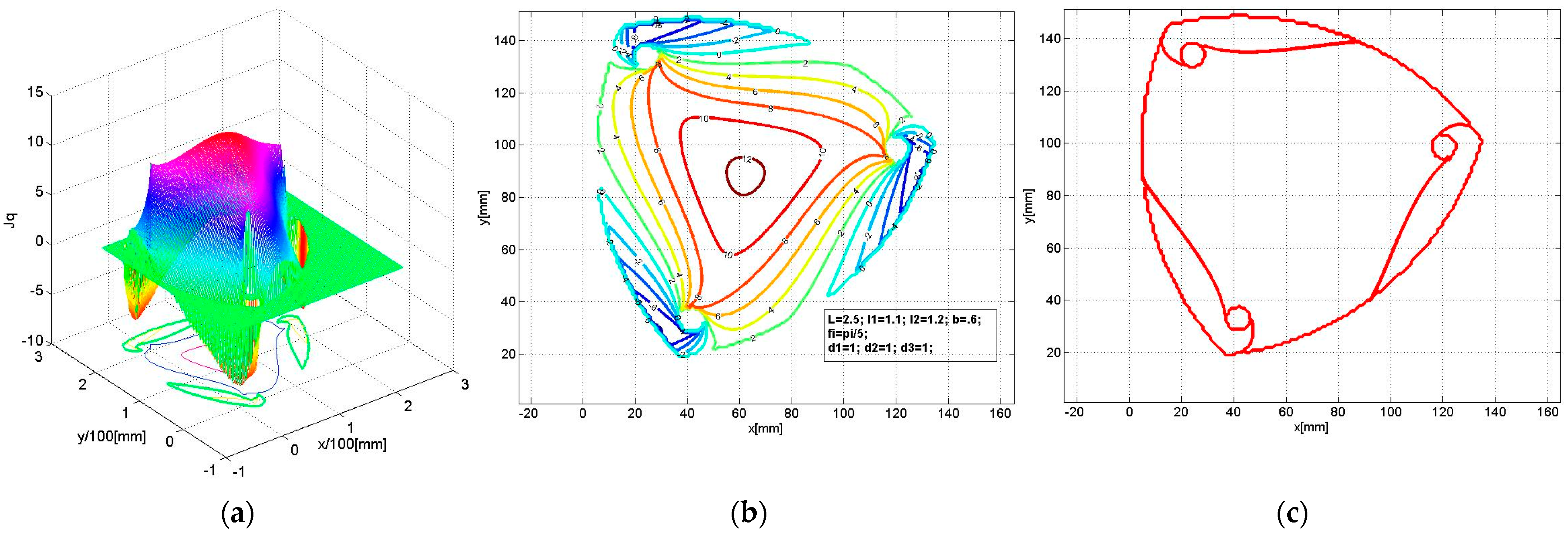
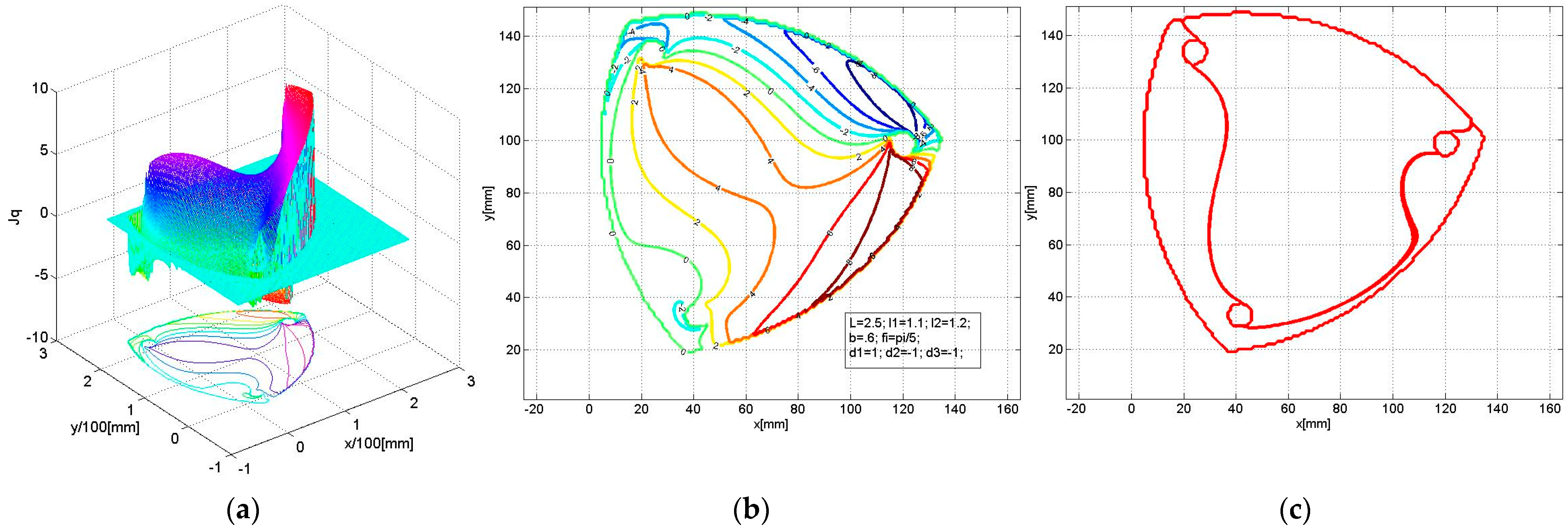
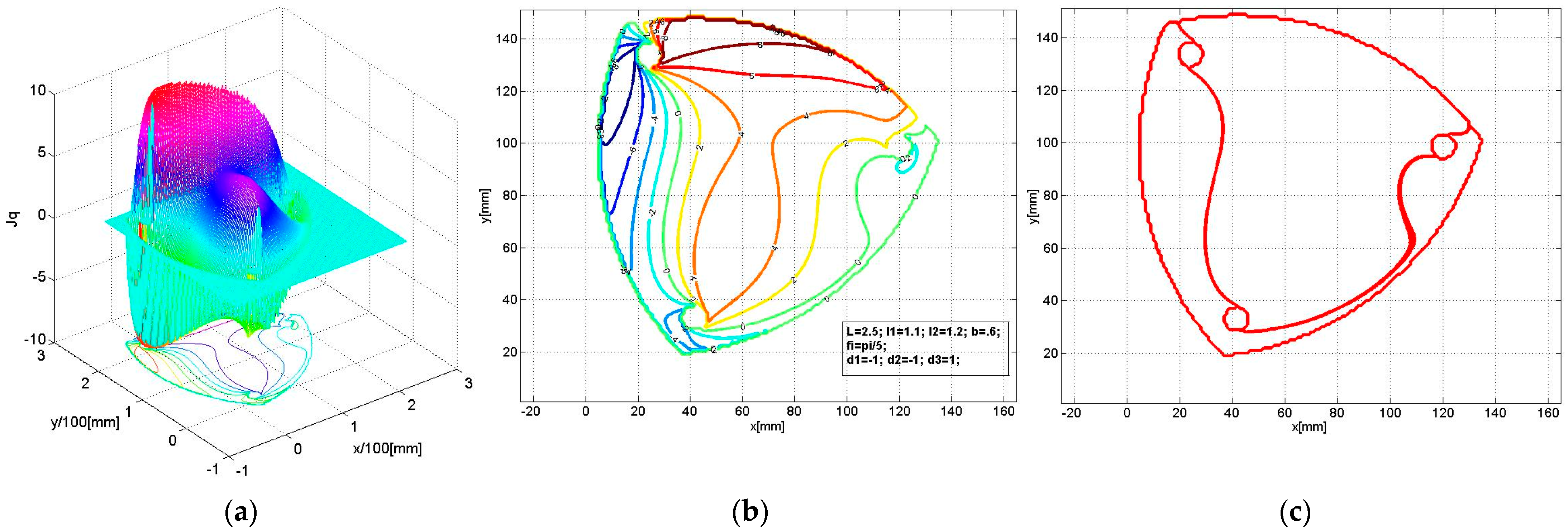
• In subfigures labeled (a), the determinant det(J_q) is illustrated as a 3D surface intersected by the plane det(J_q) = 0, which defines the singularities;
• In subfigures (b), the same surface is represented as contour lines, showing characteristic lines specific to singularities (level 0);
• In subfigures (c), only the singularity contours obtained by intersecting the surfaces with the 0-plane are shown.

Analyzing Figure 7, Figure 8, Figure 9, Figure 10, Figure 11, Figure 12, Figure 13 and Figure 14 provides important insights into the mechanism’s workspace and the singularities it exhibits. For instance, the influence of each design parameter on the presence and characteristics of singularity curves can be observed. Similarly, observations can be made regarding the eight assembly modes of the 3-RRR-type PPM, labeled in the previous section of the paper as assembly mode 1 (1, 1, 1); assembly mode 2 (1, 1, −1); assembly mode 3 (1, −1, 1); assembly mode 4 (−1, 1, 1); assembly mode 5 (1, −1, −1); assembly mode 6 (−1, 1, −1); assembly mode 7 (−1, −1, 1); and assembly mode 8 (−1, −1, −1). The influence of symmetry on these assembly modes is thus highlighted. Symmetrical assembly modes result in similar workspaces and contour curves, differing only in position, whereas asymmetrical assembly modes exhibit structural changes in both the workspace and contour curves.

6. Conclusions

This paper presents a study on the influence of the assembly mode of a 3-RRR-type PPM on its workspace, with the results representing a continuation of previous research. In this study, the authors’ work was focused on characterizing the workspace of this planar parallel manipulator, on the solutions to the inverse kinematics problem (IKP) and direct kinematics problem (DKP), as well as on the type 1 and type 2 singularities located within the workspace. All these analyses were conducted for each of the eight assembly modes of the 3-RRR-type PPM.

The results concerning the mechanism’s workspace and the solutions to the IKP and DKP problems are analytical, based on existing literature and on the authors’ prior research. The findings related to type 1 and type 2 singularities were obtained using numerical procedures.

Regarding the workspace of the 3-RRR-type PPM, it was demonstrated that the assembly mode does not influence the shape of this workspace in any way. On the contrary, the manipulator’s assembly mode has a strong influence on type 2 singularities and on the mechanism’s kinematics.

Additionally, this paper highlights the considerable variability of the workspace in relation to the dimensional characteristics of the manipulator.

A modular platform concept, suitable for experimental testing and informed by the numerical results presented here, is also proposed. The outcomes of the experimental tests will be addressed in future work.

References

1. Asada, H.; Slotine, J.J. Robot Analysis and Control; John Wiley & Sons: Hoboken, NJ, USA, 1986. [Google Scholar]
2. Fu, K.S.; Gonzalez, R.; Lee, C.S.G. Robotics: Control, Sensing, Vision, and Intelligence; McGraw-Hill: London, UK, 1987. [Google Scholar]
3. Craig, J.J. Introduction to Robotics: Mechanics and Control; Addison Wesley: Boston, UK, 1989. [Google Scholar]
4. Tsai, L.W. Robot Analysis, The Mechanics of Serial and Parallel Manipulators; John Wiley & Sons: Hoboken, NJ, USA, 1999. [Google Scholar]
5. Balan, R.; Maties, V.; Stan, S.; Lapusan, C. On the Control of a 3-RRR Planar Parallel Minirobot. J. Rom. Soc. Mechatron. 2005, 4, 20–23. [Google Scholar]
6. Racu, C.M.; Doroftei, I. Ankle rehabilitation device with two degrees of freedom and compliant joint. IOP Conf. Ser. Mater. Sci. Eng. 2015, 95, 012054. [Google Scholar] [CrossRef]
7. Racu, C.M.; Doroftei, I. An overview on ankle rehabilitation devices. Adv. Mater. Res. 2014, 1036, 781–786. [Google Scholar] [CrossRef]
8. Morar, C.A.; Doroftei, I.A.; Doroftei, I.; Hagan, M.G. Robotic applications on agricultural industry. A review. IOP Conf. Ser. Mater. Sci. Eng. 2020, 997, 12081. [Google Scholar] [CrossRef]
9. Doroftei, I.A.; Bujoreanu, C.; Doroftei, I. An overview on the applications of mechanisms in architecture. Part II: Foldable plate structures. IOP Conf. Ser. Mater. Sci. Eng. 2018, 444, 52019. [Google Scholar] [CrossRef]
10. Stewart, D. A Platform with Six Degrees of freedom. Proc. Inst. Mech. Enginners 1965, 180, 371–386. [Google Scholar] [CrossRef]
11. Dash, A.K.; Chen, I.-M.; Yeo, S.H.; Yang, G. Task-oriented configuration design for reconfigurable parallel manipulator systems. Int. J. Comput. Integr. Manuf. 2005, 18, 615–634. [Google Scholar] [CrossRef]
12. Kucuk, S. A dexterity comparison for 3-DOF planar parallel manipulators with two kinematic chains using genetic algorithms. Mechatronics 2009, 19, 868–877. [Google Scholar] [CrossRef]
13. Zhou, K.; Tao, Z.; Zhao, J.; Mao, D. Singularity loci research on high-speed travelling type of double four-rod spatial parallel mechanism. Mech. Mach. Theory 2003, 38, 195–211. [Google Scholar] [CrossRef]
14. Bhattacharya, S.; Hatwal, H.; Ghosh, A. Comparison of an exact and an approximate method of singularity avoidance in platform type parallel manipulators. Mech. Mach. Theory 1998, 33, 965–974. [Google Scholar] [CrossRef]
15. Dasgupta, B.; Mruthyunjaya, T.S. Singularity-free path planning for the Stewart platform manipulator. Mech. Mach. Theory 1998, 33, 711–725. [Google Scholar] [CrossRef]
16. Sen, S.; Dasgupta, B.; Mallik, A.K. Variational approach for singularity-free path-planning of parallel manipulators. Mech. Mach. Theory 2003, 38, 1165–1183. [Google Scholar] [CrossRef]
17. Dash, A.K.; Chen, I.M.; Yeo, S.H.; Yang, G. Workspace generation and planning singularity-free path for parallel manipulators. Mech. Mach. Theory 2005, 40, 776–805. [Google Scholar] [CrossRef]
18. Liu, S.; Qiu, Z.-C.; Zhang, X.-M. Singularity and path-planning with the working mode conversion of a 3-DOF 3-RRR planar parallel manipulator. Mech. Mach. Theory 2017, 107, 166–182. [Google Scholar] [CrossRef]
19. Bonev, I.A.; Gosselin, C.M. Singularity Loci of Planar Parallel Manipulators with Revolute Joints. In Computational Kinematics; Park, F.C., Iurascu, C.C., Eds.; Seoul, Republic of Korea, 2001; pp. 291–299. Available online: https://www.parallemic.org/Reviews/Review001.html (accessed on 31 March 2024).
20. Gosselin, C. Kinematic Analysis, Optimization and Programming of Parallel Robotic Manipulator. Ph.D Thesis, Department of Mechanical Engineering, McGill University, Montreal, QC, Canada, 1988. [Google Scholar]
21. Chablat, D.; Wenger, P. The Kinematic Analysis of a Symmetrical Three-Degree-of-Freedom Planar Parallel Manipulator. arXiv arXiv:0705.0959.
22. Doroftei, I. Singularity analysis of a 3RRR planar parallel robot I-Theoretical aspects. Bul. Institutului Politeh. Din Iaşi 2008, 54, 465–472. [Google Scholar]
23. Doroftei, I. Singularity analysis of a 3RRR planar parallel robot II-Physical significance. Bul. Institutului Politeh. Din Iaşi 2008, 54, 473–480. [Google Scholar]
24. Arsenault, M.; Boudreau, R. The synthesis of three-degree-of-freedom planar mechanism with revolute joints (3-RRR) for an optimal singularity-free workspace. J. Robot. Syst. 2004, 21, 259–274. [Google Scholar] [CrossRef]
25. Merlet, J.-P. Le Robots Paralleles, 2nd ed.; Editions Hermes: Paris, France, 1997. [Google Scholar]
26. Buium, F.; Leohchi, D.; Doroftei, I. A workspace characterization of the 3 RRR planar mechanism. Appl. Mech. Mater. 2014, 658, 563–568. [Google Scholar] [CrossRef]
27. Buium, F.; Doroftei, I. Workspace Analysis of a 3 RRR Planar Mechanism. In 25th International Symposium on Measurements and Control in Robotics, Proceedings of ISMCR 2023; Doroftei, I., Kiss, B., Baudoin, Y., Taqvi, Z., Keller Fuchter, S., Eds.; Springer: Cham, Switzerland, 2024; Mechanisms and Machine Science; Volume 154, pp. 73–82. [Google Scholar]
28. Lovasz, E.C.; Grigorescu, S.M.; Mărgineanu, D.T.; Pop, C.; Gruescu, C.M.; Maniu, I. Kinematics of the planar parallel Manipulator using Geared Linkages with linear Actuation as kinematic Chains 3-R (RPRGR) RR. In Proceedings of the 14th IFToMM World Congress, Taipei, Taiwan, 25 October 2015; pp. 25–30. [Google Scholar]
29. Lovasz, E.C.; Grigorescu, S.M.; Mărgineanu, D.T.; Pop, C.; Gruescu, C.M.; Maniu, I. Geared Linkages with Linear Actuation Used as Kinematic Chains of a Planar Parallel Manipulator. In Mechanisms, Transmissions and Applications: Proceedings of the Third MeTrApp Conference; Corves, B., Lovasz, E.C., Husing, M., Eds.; Springer: Cham, Switzerland, 2015; Mechanisms and Machine Science; Volume 31, pp. 21–31. [Google Scholar]
30. Buium, F.; Doroftei, I.; Alaci, S. Assembling Modes of a 3-RRR Planar Mechanism and Its Workspace Analysis. In Mechanism Design for Robotics. MEDER 2024; Lovasz, E.C., Ceccarelli, M., Ciupe, V., Eds.; Springer: Cham, Switzerland, 2024; Mechanisms and Machine Science; Volume 166, pp. 62–72. [Google Scholar]
Figure 1. Possible configurations of a 3DOF PPM: (a) 3-RRR configuration; (b) 3-RRP configuration; (c) 3-RPR configuration; (d) 3-PRR configuration; (e) 3-RPP configuration; (f) 3-PRP configuration; (g) 3-PPR configuration.
Robotics 14 00016 g001
Figure 2. Actuation scheme of the 3-RRR configuration: (a) 3-RRR actuation mode; (b) 3-RRR actuation mode; (c) 3-RRR actuation mode.
Robotics 14 00016 g002
Figure 3. Assembly modes of the 3RRR PPM: (a) assembly mode 1 (1, 1, 1); (b) assembly mode 2 (1, 1, −1); (c) assembly mode 3 (1, −1, 1); (d) assembly mode 4 (−1, 1, 1); (e) assembly mode 5 (1, −1, −1); (f) assembly mode 6 (−1, 1, −1); (g) assembly mode 7 (−1, −1, 1); (h) assembly mode 8 (−1, −1, −1).
Robotics 14 00016 g003
Figure 4. Schematic design of 3-RRR PPM.
Robotics 14 00016 g004
Figure 5. Superposed workspaces of the 3-RRR PPM obtained by (a) varying L; (b) varying b, φ = π / 10 ; (c) varying b, φ = π / 2 ; (d) varying l 1 ; (e) varying l 2 ; and (f) varying φ .
Robotics 14 00016 g005
Figure 6. Schema of the applied methodology [27].
Robotics 14 00016 g006
Figure 7. Workspace for the 1st assembly mode (1, 1, 1): (a) values of det(Jq); (b) level curves; (c) workspace.
Robotics 14 00016 g007
Figure 8. Workspace for the 3rd assembly mode (1, 1, −1): (a) values of det(Jq); (b) level curves; (c) workspace.
Robotics 14 00016 g008
Figure 9. Workspace for the 6th assembly mode (1, −1, 1): (a) values of det(Jq); (b) level curves; (c) workspace.
Robotics 14 00016 g009
Figure 10. Workspace for the 2nd assembly mode (−1, 1, 1): (a) values of det(Jq); (b) level curves; (c) workspace.
Robotics 14 00016 g010
Figure 11. Workspace for the 8th assembly mode (1, −1, −1): (a) values of det(Jq); (b) level curves; (c) workspace.
Robotics 14 00016 g011
Figure 12. Workspace for the 4th assembly mode (−1, 1, −1): (a) values of det(Jq); (b) level curves; (c) workspace.
Robotics 14 00016 g012
Figure 13. Workspace for the 5th assembly mode (−1, −1, 1): (a) values of det(Jq); (b) level curves; (c) workspace.
Robotics 14 00016 g013
Figure 14. Workspace for the 7th assembly mode (−1, −1, −1): (a) values of det(Jq); (b) level curves; (c) workspace.
Robotics 14 00016 g014
Figure 15. Experimental platform of the 3-RRR PPM: (a) 3D CAD design; (b) real platform [30].
Robotics 14 00016 g015
Figure 16. Actuation modes of the platform (actuator in red color): (a) 3-RRR actuation mode; (b) 3-RRR actuation mode; (c) 3-RRR actuation mode.
Robotics 14 00016 g016
Figure 17. Assembly modes of the proposed platform, according to Figure 3: (a) assembly mode 1 (1, 1, 1); (b) assembly mode 2 (1, 1, −1); (c) assembly mode 3 (1, −1, 1); (d) assembly mode 4 (−1, 1, 1); (e) assembly mode 5 (1, −1, −1); (f) assembly mode 6 (−1, 1, −1); (g) assembly mode 7 (−1, −1, 1); (h) assembly mode 8 (−1, −1, −1).
Robotics 14 00016 g017
Figure 18. Modification of the constructive parameters ( l 1 and l 2 ) of the kinematic chain that connects the final effector to the base: (a) l 1 and l 2 have minimum values ( l 1 = l 2 = 108   [mm]); (b) l 1 and l 2 have maximum values ( l 1 = l 2 = 133   [mm]).
Robotics 14 00016 g018
Figure 19. Different configurations of the platform, based on the range of the constructive parameters: (a) variant 1 ( l 1 = l 2 = 108   [mm], L = 305   [mm], b = 75   [mm]); (b) variant 2 ( l 1 = l 2 = 108   [mm], L = 440   [mm], b = 160   [mm]); (c) variant 3 ( l 1 = l 2 = 133   [mm], L = 305   [mm], b = 75   [mm]); (d) variant 4 ( l 1 = l 2 = 133   [mm], L = 440   [mm], b = 160   [mm]); (e) variant 5 ( l 1 = 133   [mm], l 2 = 108   [mm], L = 305   [mm], b = 75   [mm]); (f) variant 6 ( l 1 = 133   [mm], l 2 = 108   [mm], L = 440   [mm], b = 160   [mm]); (g) variant 7 ( l 1 = 108   [mm], l 2 = 133   [mm], L = 305   [mm], b = 75   [mm]); (h) variant 8 ( l 1 = 108   [mm], l 2 = 133   [mm], L = 440   [mm], b = 160   [mm]).
Robotics 14 00016 g019
Disclaimer/Publisher’s Note: The statements, opinions and data contained in all publications are solely those of the individual author(s) and contributor(s) and not of MDPI and/or the editor(s). MDPI and/or the editor(s) disclaim responsibility for any injury to people or property resulting from any ideas, methods, instructions or products referred to in the content.