
3D Point Cloud Data in Conveying Information for Local Green Factor Assessment

 , , , ,
Abstract
:1. Introduction
2. Materials and Methods
2.1. Study Site, Measurements, and Data Sets
2.1.1. Tarot T960
2.1.2. DJI Phantom 4 Pro+
2.1.3. Leica RTC360
2.1.4. GeoSLAM ZEB Revo RT
2.2. Green Factor Elements
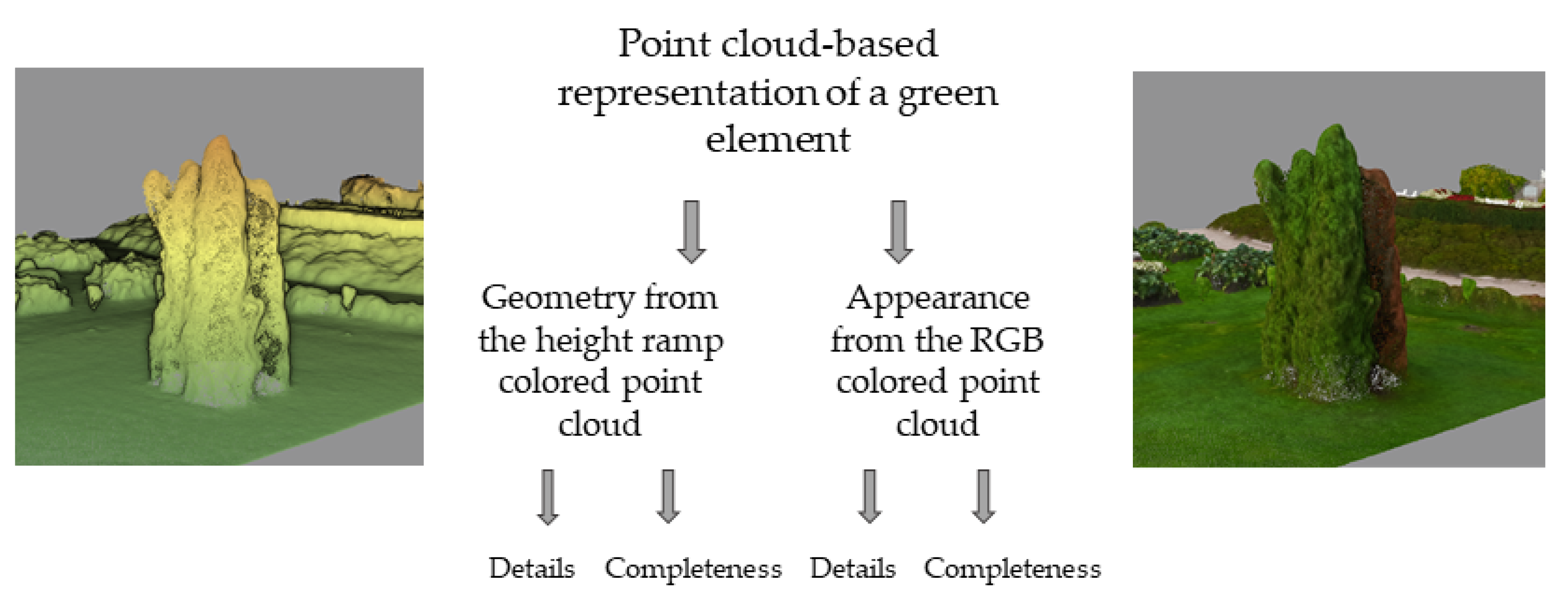
2.3. Study Design
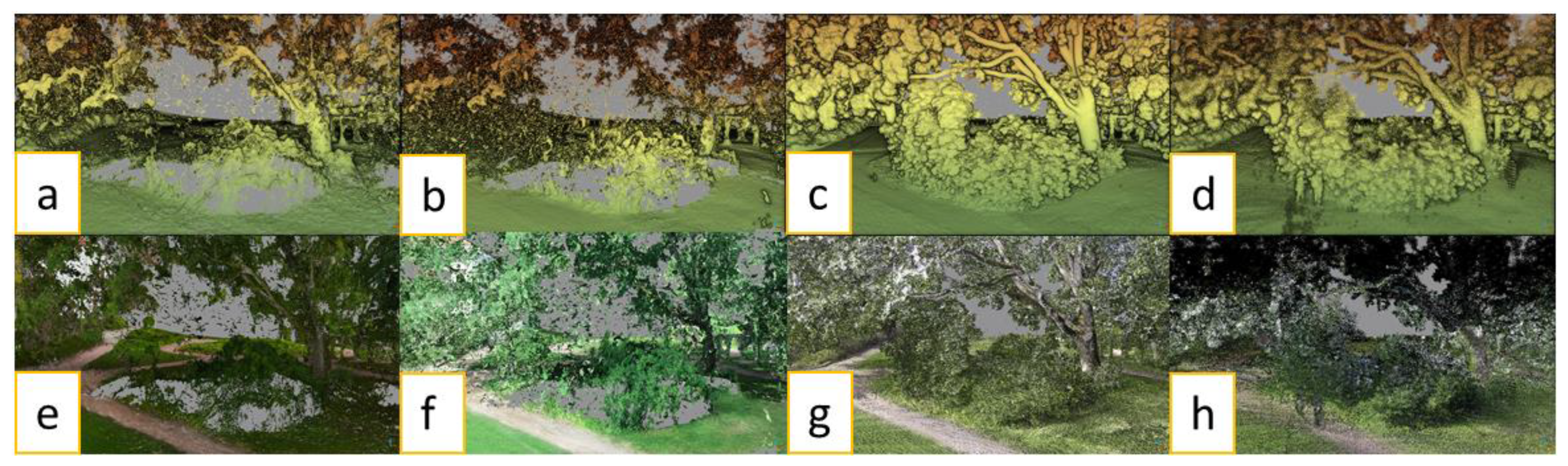
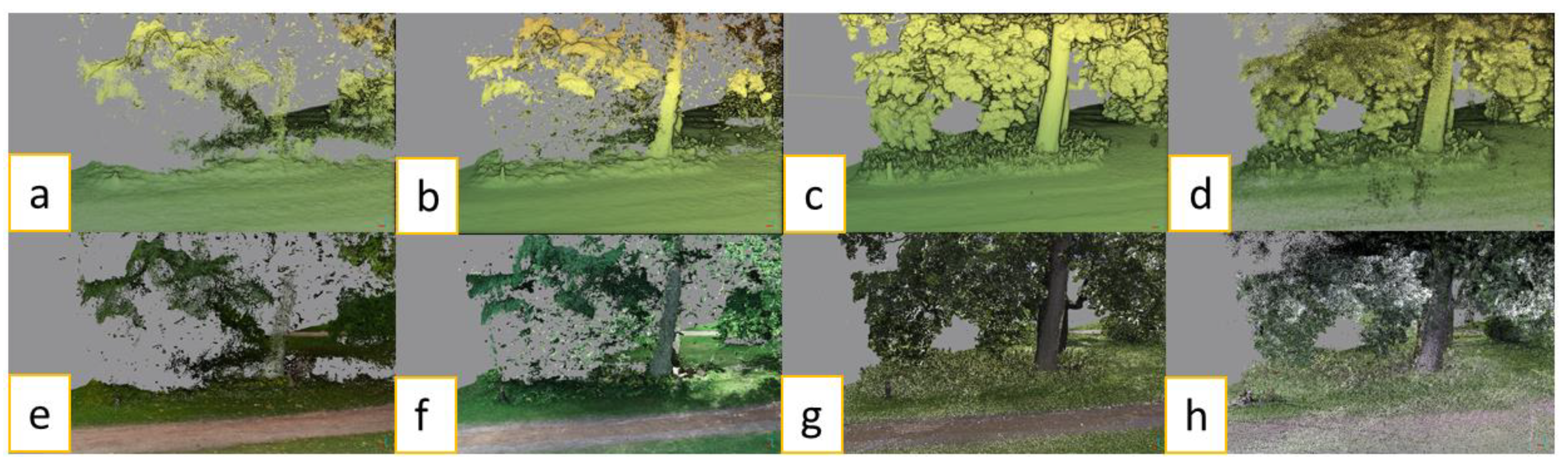
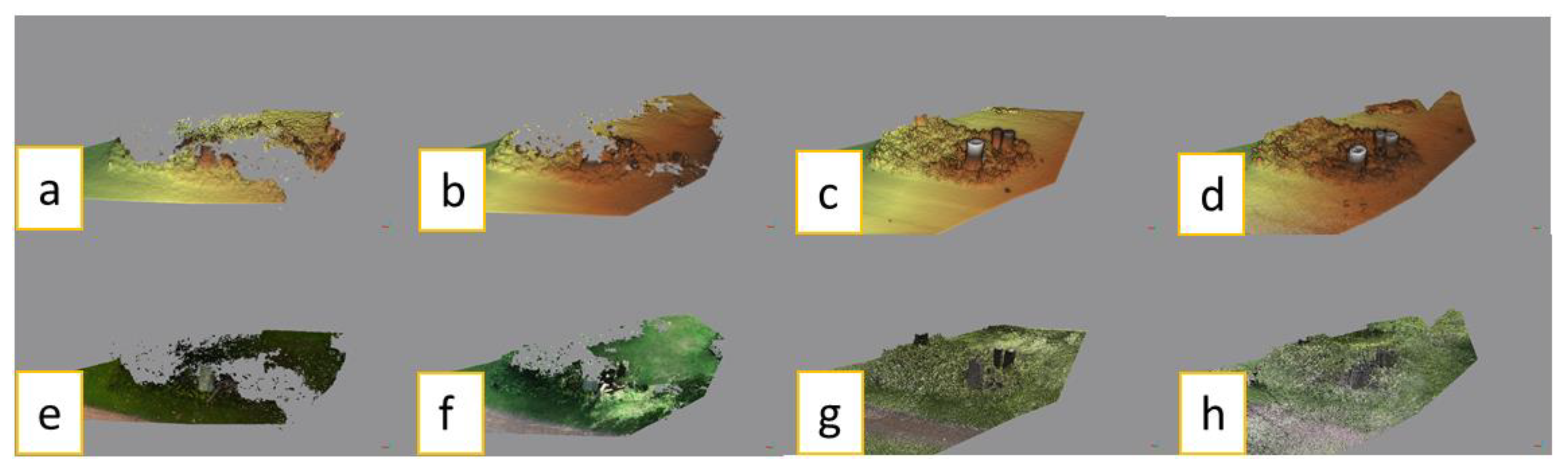
3. Results
4. Discussion
4.1. Suitability of Point Cloud-Based Information for the Purposes of Monitoring Local Green Elements
4.2. Differences of Data Acquisition Methods
4.3. Prospects for the Point Cloud-Based Evaluation of the Local Existing Green Factor
4.4. Remarks on the Study Design and Future Research
5. Conclusions
Author Contributions
Funding
Conflicts of Interest
Appendix A

| Element Group | Element Description |
|---|---|
| Stormwater management solutions | Rain garden (biofiltration area) with a broad range of layered |
| Infiltration pit (underground) | |
| Retention or detention basin or swale covered with vegetation or aggregates (permeable soil) | |
| Retention or detention pit, tank or cistern (underground, notice units: volume!) | |
| Biofiltration basin or swale | |
| Bonus elements | Capturing stormwater from impermeable surfaces for use in irrigation or directing it in a controlled manner to permeable vegetated areas |
| Directing stormwater from impermeable surfaces to constructed water features, such as ponds and streams, with flowing water | |
| Preserved vegetation and soil | Preserved natural meadow or natural ground vegetation |
| Preserved natural bare rock area (at least partially bare rock surface, not many trees) | |
| Planted/new vegetation | Meadow or dry meadow |
| Cultivation plots | |
| Green wall, vertical area | |
| Pavements | Impermeable surface |
| Stormwater management solutions | Intensive green roof/roof garden, depth of substrate 20–100 cm |
| Semi-intensive green roof, depth of substrate 15–30 cm | |
| Extensive green roof, depth of substrate 6–8 cm | |
| Pond, wetland or water meadow with natural vegetation (permanent water surface at least part of the year; at other times the ground remains moist) | |
| Bonus elements | Fruit trees or berry bushes suitable for cultivation (10 m2 each) |
| Boxes for urban farming/cultivation | |
| Permeable surface designated for play or sports (e.g., sand- or gravel-covered playgrounds, sports turf) | |
| Communal rooftop gardens or balconies with at least 10% of the total area covered by vegetation |
Appendix B
| Element Group (in the Original Green Factor) | Element Description (in the Original Green Factor) | Unit (in the Original Green Factor) | Potential to Utilize Point Clouds as Part of the Existing Green Factor Assessment (Tentative Estimation) |
|---|---|---|---|
| Preserved vegetation and soil | Preserved large (fully grown > 10 m) tree in good condition, at least 3 m (25 m2 each) | pcs | Yes |
| Preserved small (fully grown ≤ 10 m) tree in good condition, at least 3 m (15 m2 each) | pcs | Yes | |
| Preserved tree in good condition (1.5–3 m) or a large shrub (3 m2 each) | pcs | Yes | |
| Preserved natural meadow or natural ground vegetation | m2 | Yes | |
| Preserved natural bare rock area (at least partially bare rock surface, not many trees) | m2 | Yes | |
| Planted/new vegetation | Large tree species, fully grown > 10 m (25 m2 each) | pcs | Yes |
| Small tree species, fully grown ≤ 10 m (15 m2 each) | pcs | Yes | |
| Large shrubs (3 m2 each) | pcs | Yes | |
| Other shrubs | m2 | Yes | |
| Perennials | m2 | Yes | |
| Meadow or dry meadow | m2 | No, or only as supportive source | |
| Cultivation plots | m2 | Needs verification | |
| Lawn | m2 | Yes | |
| Perennial vines (2 m2 each) | pcs | Yes | |
| Green wall, vertical area | m2 | Yes | |
| Pavements | Semipermeable pavements (e.g., grass stones, stone ash) | m2 | No, or only as supportive source |
| Permeable pavements (e.g., gravel and sand surfaces) | m2 | No, or only as supportive source | |
| Impermeable surface | m2 | No, or only as supportive source | |
| Stormwater management solutions | Rain garden (biofiltration area) with a broad range of layered vegetation | m2 | No, or only as supportive source |
| Intensive green roof/roof garden, depth of substrate 20–100 cm | m2 | Needs verification | |
| Semi-intensive green roof, depth of substrate 15–30 cm | m2 | Needs verification | |
| Extensive green roof, depth of substrate 6–8 cm | m2 | Needs verification | |
| Infiltration basin or swale covered with vegetation or aggregates (no permanent pool of water, permeable soil) | m2 | No, or only as supportive source | |
| Infiltration pit (underground) | m2 | No, or only as supportive source | |
| Pond, wetland or water meadow with natural vegetation (permanent water surface at least part of the year; at other times the ground remains moist) | m2 | Needs verification | |
| Retention or detention basin or swale covered with vegetation or aggregates (permeable soil) | m2 | No, or only as supportive source | |
| Retention or detention pit, tank or cistern (underground, notice units: volume!) | m3 | No, or only as supportive source | |
| Biofiltration basin or swale | m2 | No, or only as supportive source | |
| Bonus elements, max score 1 per category | Capturing stormwater from impermeable surfaces for use in irrigation or directing it in a controlled manner to permeable vegetated areas | m2 | No, or only as supportive source |
| Directing stormwater from impermeable surfaces to constructed water features, such as ponds and streams, with flowing water | m2 | No, or only as supportive source | |
| Shading large tree (25 m2 each) on the south or southwest side of the building (especially deciduous trees) | pcs | Yes | |
| Shading small tree (15 m2 each) on the south or southwest side of the building (especially deciduous trees) | pcs | Yes | |
| Fruit trees or berry bushes suitable for cultivation (10 m2 each) | pcs | No, or only as supportive source | |
| A selection of native species—at least 5 species/100 m2 | m2 | Needs verification | |
| Tree species native to Helsinki and flowering trees and shrubs—at least 3 species/100 m2 | m2 | Needs verification | |
| Butterfly meadows or plants with pleasant scent or impressive blooming | m2 | Needs verification | |
| Boxes for urban farming/cultivation | m2 | Needs verification | |
| Permeable surface designated for play or sports (e.g., sand- or gravel-covered playgrounds, sports turf) | m2 | No, or only as supportive source | |
| Communal rooftop gardens or balconies with at least 10% of the total area covered by vegetation | m2 | Yes | |
| Structures supporting natural and/or animal living conditions such as preserved dead wood/stumps or birdboxes (5 m2 each) | pcs | Needs verification |
References
- World Health Organization. Ecosystems and Human Well-Being: Health Synthesis: A Report of the Millennium Ecosystem Assessment; World Health Organization: Geneva, Switzerland, 2007. [Google Scholar]
- European Commission. Communication from the Commission to the European Parliament, the Council, the European Economic and Social Committee and the Committee of the Regions. In Green Infrastructure (GI)—Enhancing Europe’s Natural Capital; COM (2013) 249 Final; European Commission: Brussels, Belgium, 2013. [Google Scholar]
- Faehnle, M.E. ViherKARA. Kaupunkiseutujen vihreän infrastruktuurin käsitteitä. In Suomen Ympäristökeskuksen Raportteja 39/2013; Suomen ympäristökeskus: Helsinki, Finland, 2013. [Google Scholar]
- Cameron, R.W.; Blanuša, T.; Taylor, J.E.; Salisbury, A.; Halstead, A.J.; Henricot, B.; Thompson, K. The domestic garden–Its contribution to urban green infrastructure. Urban For. Urban Green. 2012, 11, 129–137. [Google Scholar] [CrossRef]
- Organisation for Economic Co-operation and Development. Compact City Policies: A Comparative Assessment; OECD: Pairs, France, 2012. [Google Scholar]
- Tsunetsugu, Y.; Lee, J.; Park, B.J.; Tyrväinen, L.; Kagawa, T.; Miyazaki, Y. Physiological and psychological effects of viewing urban forest landscapes assessed by multiple measurements. Landsc. Urban Plan. 2013, 113, 90–93. [Google Scholar] [CrossRef]
- Grahn, P.; Stigsdotter, U.K. The relation between perceived sensory dimensions of urban green space and stress restoration. Landsc. Urban Plan. 2012, 94, 264–275. [Google Scholar] [CrossRef]
- Tyrväinen, L.; Mäkinen, K.; Schipperijn, J. Tools for mapping social values of urban woodlands and other green areas. Landsc. Urban Plan. 2007, 79, 5–19. [Google Scholar] [CrossRef]
- Venter, Z.S.; Barton, D.N.; Gundersen, V.; Figari, H.; Nowell, M. Urban nature in a time of crisis: Recreational use of green space increases during the COVID-19 outbreak in Oslo, Norway. Environ. Res. Lett. 2020, 15, 104075. [Google Scholar] [CrossRef]
- Jackson, S.B.; Stevenson, K.T.; Larson, L.R.; Peterson, M.N.; Seekamp, E. Outdoor activity participation improves adolescents’ mental health and well-being during the COVID-19 pandemic. Int. J. Environ. Res. Public Health 2021, 18, 2506. [Google Scholar] [CrossRef]
- Fagerholm, N.; Eilola, S.; Arki, V. Outdoor recreation and nature’s contribution to well-being in a pandemic situation-Case Turku, Finland. Urban For. Urban Green. 2021, 64, 127257. [Google Scholar] [CrossRef]
- Wolch, J.R.; Byrne, J.; Newell, J.P. Urban green space, public health, and environmental justice: The challenge of making cities ‘just green enough’. Landsc. Urban Plan. 2014, 125, 234–244. [Google Scholar] [CrossRef] [Green Version]
- Rigolon, A.; Németh, J. “We’re not in the business of housing:” Environmental gentrification and the non-profitization of green infrastructure projects. Cities 2018, 81, 71–80. [Google Scholar] [CrossRef]
- Ojala, A.; Niemelä, J.; Yli-Pelkonen, V. Impacts of residential infilling on private gardens in the Helsinki Metropolitan Area. In Green Landscapes in the European City, 1750–2010; Clark, P., Niemi, M., Nolin, C., Eds.; Routledge Studies in Modern European History; Routledge: London, UK; New York, NY, USA, 2017; pp. 71–86. [Google Scholar]
- Ariluoma, M.; Ottelin, J.; Hautamäki, R.; Tuhkanen, E.M.; Mänttäri, M. Carbon sequestration and storage potential of urban green in residential yards: A case study from Helsinki. Urban For. Urban Green. 2021, 57, 126939. [Google Scholar] [CrossRef]
- Loram, A.; Tratalos, J.; Warren, P.H.; Gaston, K.J. Urban domestic gardens (X): The extent & structure of the resource in five major cities. Landsc. Ecol. 2007, 22, 601–615. [Google Scholar]
- Clark, C.; Ordóñez, C.; Livesley, S.J. Private tree removal, public loss: Valuing and enforcing existing tree protection mechanisms is the key to retaining urban trees on private land. Landsc. Urban Plan. 2020, 203, 103899. [Google Scholar] [CrossRef]
- Bush, J.; Ashley, G.; Foster, B.; Hall, G. Integrating Green Infrastructure into Urban Planning: Developing Melbourne’s Green Factor Tool. Urban Plan. 2021, 6, 20–31. [Google Scholar] [CrossRef]
- Keeley, M. The Green Area Ratio: An urban site sustainability metric. J. Environ. Plan. Manag. 2011, 54, 937–958. [Google Scholar] [CrossRef]
- Juhola, S. Planning for a green city: The Green Factor tool. Urban For. Urban Green. 2018, 34, 254–258. [Google Scholar] [CrossRef]
- Stenning, E. An Assessment of the Seattle Green Factor: Increasing and Improving the Quality of Urban Green Infrastructure. Master’s Thesis, University of Washington, Seattle, WA, USA, 2008. [Google Scholar]
- Inkiläinen, E.; Tiihonen, T.; Eitsi, E. Viherkerroinmenetelmän kehittäminen Helsingin kaupungille. In Helsingin Kaupungin Ympäristökeskuksen Julkaisuja 8/2014; Helsingin kaupungin ympäristökeskus: Helsinki, Finland, 2014. [Google Scholar]
- Helsinki City Council. Viherkertoimen Käyttö Viihtyvyyden, Sopeutumisen Ja Luonnon Monimuotoisuuden Edistämiseksi; Helsinki City Council: Helsinki, Finland, 2020. [Google Scholar]
- Yu, X.; Hyyppä, J.; Karjalainen, M.; Nurminen, K.; Karila, K.; Vastaranta, M.; Kankare, V.; Kaartinen, H.; Holopainen, M.; Honkavaara, E.; et al. Comparison of laser and stereo optical, SAR and InSAR point clouds from air-and space-borne sources in the retrieval of forest inventory attributes. Remote Sens. 2015, 7, 15933–15954. [Google Scholar] [CrossRef] [Green Version]
- Puliti, S.; Gobakken, T.; Ørka, H.O.; Næsset, E. Assessing 3D point clouds from aerial photographs for species-specific forest inventories. Scand. J. For. Res. 2017, 32, 68–79. [Google Scholar] [CrossRef]
- White, J.C.; Stepper, C.; Tompalski, P.; Coops, N.C.; Wulder, M.A. Comparing ALS and image-based point cloud metrics and modelled forest inventory attributes in a complex coastal forest environment. Forests 2015, 6, 3704–3732. [Google Scholar] [CrossRef]
- Al-Rawabdeh, A.; He, F.; Moussa, A.; El-Sheimy, N.; Habib, A. Using an unmanned aerial vehicle-based digital imaging system to derive a 3D point cloud for landslide scarp recognition. Remote Sens. 2016, 8, 95. [Google Scholar] [CrossRef] [Green Version]
- Yonglin, S.; Lixin, W.; Zhi, W. Identification of inclined buildings from aerial lidar data for disaster management. In Proceedings of the 2010 18th International Conference on Geoinformatics, Beijing, China, 18–20 June 2010; pp. 1–5. [Google Scholar]
- Chen, Z.; Xu, B.; Devereux, B. Urban landscape pattern analysis based on 3D landscape models. Appl. Geogr. 2014, 55, 82–91. [Google Scholar] [CrossRef]
- Urech, P.R.; Dissegna, M.A.; Girot, C.; Grêt-Regamey, A. Point cloud modeling as a bridge between landscape design and planning. Landsc. Urban Plan. 2020, 203, 103903. [Google Scholar] [CrossRef]
- Vosselman, G. Point cloud segmentation for urban scene classification. Int. Arch. Photogramm. Remote Sens. Spat. Inf. Sci. 2013, 1, 257–262. [Google Scholar] [CrossRef] [Green Version]
- Safaie, A.H.; Rastiveis, H.; Shams, A.; Sarasua, W.A.; Li, J. Automated street tree inventory using mobile LiDAR point clouds based on Hough transform and active contours. ISPRS J. Photogramm. Remote Sens. 2021, 174, 19–34. [Google Scholar] [CrossRef]
- Weinmann, M.; Weinmann, M.; Mallet, C.; Brédif, M. A classification-segmentation framework for the detection of individual trees in dense MMS point cloud data acquired in urban areas. Remote Sens. 2017, 9, 277. [Google Scholar] [CrossRef] [Green Version]
- Cabo, C.; Ordoñez, C.; García-Cortés, S.; Martínez, J. An algorithm for automatic detection of pole-like street furniture objects from Mobile Laser Scanner point clouds. ISPRS J. Photogramm. Remote Sens. 2014, 87, 47–56. [Google Scholar] [CrossRef]
- Lin, X.; Yang, B.; Wang, F.; Li, J.; Wang, X. Dense 3D surface reconstruction of large-scale streetscape from vehicle-borne imagery and LiDAR. Int. J. Digit. Earth 2021, 14, 619–639. [Google Scholar] [CrossRef]
- Neuville, R.; Bates, J.S.; Jonard, F. Estimating forest structure from UAV-mounted LiDAR point cloud using machine learning. Remote Sens. 2021, 13, 352. [Google Scholar] [CrossRef]
- Bottalico, F.; Chirici, G.; Giannini, R.; Mele, S.; Mura, M.; Puxeddu, M.; McRoberts, R.E.; Valbuena, R.; Travaglini, D. Modeling Mediterranean forest structure using airborne laser scanning data. Int. J. Appl. Earth Obs. Geoinf. 2017, 57, 145–153. [Google Scholar] [CrossRef]
- Wallace, L.; Hillman, S.; Reinke, K.; Hally, B. Non-destructive estimation of above-ground surface and near-surface biomass using 3D terrestrial remote sensing techniques. Methods Ecol. Evol. 2017, 8, 1607–1616. [Google Scholar] [CrossRef] [Green Version]
- Carr, J.C.; Slyder, J.B. Individual tree segmentation from a leaf-off photogrammetric point cloud. Int. J. Remote Sens. 2018, 39, 5195–5210. [Google Scholar] [CrossRef]
- Kaartinen, H.; Hyyppä, J.; Yu, X.; Vastaranta, M.; Hyyppä, H.; Kukko, A.; Holopainen, M.; Heipke, C.; Hirschmugl, M.; Morsdorf, F.; et al. An international comparison of individual tree detection and extraction using airborne laser scanning. Remote Sens. 2012, 4, 950–974. [Google Scholar] [CrossRef] [Green Version]
- Nevalainen, O.; Honkavaara, E.; Tuominen, S.; Viljanen, N.; Hakala, T.; Yu, X.; Hyyppä, J.; Saari, H.; Pölönen, I.; Imai, N.N.; et al. Individual tree detection and classification with UAV-based photogrammetric point clouds and hyperspectral imaging. Remote Sens. 2017, 9, 185. [Google Scholar] [CrossRef] [Green Version]
- Saarinen, N.; Calders, K.; Kankare, V.; Yrttimaa, T.; Junttila, S.; Luoma, V.; Huuskonen, S.; Hynynen, J.; Verbeeck, H. Understanding 3D structural complexity of individual Scots pine trees with different management history. Ecol. Evol. 2021, 11, 2561–2572. [Google Scholar] [CrossRef]
- Zhang, C.; Zhou, Y.; Qiu, F. Individual tree segmentation from LiDAR point clouds for urban forest inventory. Remote Sens. 2015, 7, 7892–7913. [Google Scholar] [CrossRef] [Green Version]
- Yu, X.; Hyyppä, J.; Kaartinen, H.; Maltamo, M. Automatic detection of harvested trees and determination of forest growth using airborne laser scanning. Remote Sens. Environ. 2004, 90, 451–462. [Google Scholar] [CrossRef]
- Hyyppä, J.; Xiaowei, Y.; Rönnholm, P.; Kaartinen, H.; Hyyppä, H. Factors affecting object-oriented forest growth estimates obtained using laser scanning. Photogramm. J. Finl. 2003, 18, 16–31. [Google Scholar]
- Tompalski, P.; Coops, N.C.; White, J.C.; Goodbody, T.R.; Hennigar, C.R.; Wulder, M.A.; Socha, J.; Woods, M.E. Estimating Changes in Forest Attributes and Enhancing Growth Projections: A Review of Existing Approaches and Future Directions Using Airborne 3D Point Cloud Data. Curr. For. Rep. 2021, 7, 1–24. [Google Scholar]
- Liang, X.; Kankare, V.; Hyyppä, J.; Wang, Y.; Kukko, A.; Haggrén, H.; Yu, X.; Kaartinen, H.; Jaakkola, A.; Guan, F.; et al. Terrestrial laser scanning in forest inventories. ISPRS J. Photogramm. Remote Sens. 2016, 115, 63–77. [Google Scholar] [CrossRef]
- Casalegno, S.; Anderson, K.; Cox, D.T.; Hancock, S.; Gaston, K.J. Ecological connectivity in the three-dimensional urban green volume using waveform airborne lidar. Sci. Rep. 2017, 7, 45571. [Google Scholar]
- Alavipanah, S.; Haase, D.; Lakes, T.; Qureshi, S. Integrating the third dimension into the concept of urban ecosystem services: A review. Ecol. Indic. 2017, 72, 374–398. [Google Scholar] [CrossRef]
- Feltynowski, M.; Kronenberg, J.; Bergier, T.; Kabisch, N.; Łaszkiewicz, E.; Strohbach, M.W. Challenges of urban green space management in the face of using inadequate data. Urban For. Urban Green. 2018, 31, 56–66. [Google Scholar] [CrossRef]
- Larkin, A.; Hystad, P. Evaluating street view exposure measures of visible green space for health research. J. Expo. Sci. Environ. Epidemiol. 2019, 29, 447–456. [Google Scholar] [CrossRef] [PubMed]
- City of Espoo. Träskändan Kartanopuiston Hoito-Ja Käyttösuunnitelma 2018–2028; City of Espoo: Espoo, Finland, 2017. [Google Scholar]
- Kauhanen, H.; Rönnholm, P.; Vaaja, M.; Hyyppä, H. Designing and building a cost-efficient survey drone. Int. Arch. Photogramm. Remote Sens. Spat. Inf. Sci. 2020, 43, 165–172. [Google Scholar] [CrossRef]
- DJI. Phantom 4 Pro. 2021. Available online: https://www.dji.com/fi/phantom-4-pro (accessed on 1 September 2021).
- Leica. Leica RTC360 3D Laser Scanner. 2021. Available online: https://leica-geosystems.com/products/laser-scanners/scanners/leica-rtc360 (accessed on 1 September 2021).
- GeoSLAM. Zeb Revo RT Capture with Confidence. 2021. Available online: https://mzt1b2rcaay128n901d0fifo-wpengine.netdna-ssl.com/wp-content/uploads/2020/08/ZEB-Revo-RT-product-card-1.pdf (accessed on 1 September 2021).
- GeoSLAM. Zeb-Revo RT User’s Manual. 2018. Available online: https://geoslam.com/wp-content/uploads/2021/02/ZEB-REVO-RT-User-Guide-V1-0-3.pdf (accessed on 1 September 2021).
- GeoSLAM. Zeb-CAM User Guide. Available online: https://download.geoslam.com/docs/zeb-cam/ZEB-CAM%20User%20Guide%20V1-0-1.pdf (accessed on 1 September 2021).
- iWater Project. About iWater Project. Available online: https://www.integratedstormwater.eu/about (accessed on 1 September 2021).
- iWater Project. Green Factor Tool. Available online: https://www.integratedstormwater.eu/sites/www.integratedstormwater.eu/files/final_outputs/green_factor_tool_protected.xlsm (accessed on 1 September 2021).
- Saran, S.; Oberai, K.; Wate, P.; Konde, A.; Dutta, A.; Kumar, K.; Kumar, A.S. Utilities of virtual 3D city models based on CityGml: Various use cases. J. Indian Soc. Remote Sens. 2018, 46, 957–972. [Google Scholar] [CrossRef]
- Julin, A.; Kurkela, M.; Rantanen, T.; Virtanen, J.P.; Maksimainen, M.; Kukko, A.; Kaartinen, H.; Vaaja, M.T.; Hyyppä, J.; Hyyppä, H. Evaluating the quality of TLS point cloud colorization. Remote Sens. 2020, 12, 2748. [Google Scholar] [CrossRef]
- Richard, A. From Point Clouds to High-Fidelity Models-Advanced Methods for Image-Based 3D Reconstruction. Doctoral Dissertation, ETH Zurich, Zurich, Switzerland, 2021. [Google Scholar]
- CloudCompare. 3D Point Cloud and Mesh Processing Software. 2021. Available online: http://www.cloudcompare.org/ (accessed on 1 September 2021).
- CloudCompare. CloudCompare Wiki. 2016. Available online: https://www.cloudcompare.org/doc/wiki/index.php?title=Main_Page (accessed on 1 September 2021).
- Kersten, T.P.; Mechelke, K.; Lindstaedt, M.; Sternberg, H. Methods for geometric accuracy investigations of terrestrial laser scanning systems. Photogramm. Fernerkund. Geoinf. 2009, 4, 301–315. [Google Scholar] [CrossRef] [PubMed]
- Tucci, G.; Visintini, D.; Bonora, V.; Parisi, E.I. Examination of Indoor Mobile Mapping Systems in a Diversified Internal/External Test Field. Appl. Sci. 2018, 8, 401. [Google Scholar] [CrossRef] [Green Version]
- Sirmaceka, B.; Shena, Y.; Lindenbergha, R.; Zlatanovab, S.; Diakiteb, A. Comparison of ZEB1 and Leica C10 indoor laser scanning point clouds. ISPRS Ann. Photogramm. Remote Sens. Spat. Inf. Sci. 2016, 3, 143–149. [Google Scholar] [CrossRef] [Green Version]
- Chiabrando, F.; Della Coletta, C.; Sammartano, G.; Spanò, A.; Spreafico, A. “Torino 1911” project: A Contribution of a SLAM-based Survey to Extensive 3D Heritage Modelling. Int. Arch. Photogramm. Remote Sens. Spat. Inf. Sci. 2018, 42, 225–234. [Google Scholar] [CrossRef] [Green Version]
- Filippo, A.; Sánchez-Aparicio, L.J.; Barba, S.; Martín-Jiménez, J.A.; Mora, R.; González Aguilera, D. Use of a wearable mobile laser system in seamless indoor 3d mapping of a complex historical site. Remote Sens. 2018, 10, 1897. [Google Scholar] [CrossRef] [Green Version]
- Frangez, V.; Kramis, B.; Hübscher, F.; Baumann, A. Comparison of Three Innovative Technologies for 3D-Acquisition, Modelling, and Visualization of an Underground Mine. In FIG Congress 2018 Online Proceedings 2018; International Federation of Surveyors (FIG): Paris, France, 2018; p. 9502. [Google Scholar]
- Pomerleau, F.; Liu, M.; Colas, F.; Siegwart, R. Challenging data sets for point cloud registration algorithms. Int. J. Robot. Res. 2012, 31, 1705–1711. [Google Scholar] [CrossRef] [Green Version]
- Nex, F.; Remondino, F. UAV for 3D mapping applications: A review. Appl. Geomat. 2014, 6, 1–15. [Google Scholar] [CrossRef]
- Hyyppä, E.; Hyyppä, J.; Hakala, T.; Kukko, A.; Wulder, M.A.; White, J.C.; Pyörälä, J.; Yu, X.; Wang, Y.; Virtanen, J.P.; et al. Under-canopy UAV laser scanning for accurate forest field measurements. ISPRS J. Photogramm. Remote Sens. 2020, 164, 41–60. [Google Scholar] [CrossRef]
- Morgenthal, G.; Hallermann, N. Quality assessment of unmanned aerial vehicle (UAV) based visual inspection of structures. Adv. Struct. Eng. 2014, 17, 289–302. [Google Scholar] [CrossRef]
- Li, L.; Mu, X.; Soma, M.; Wan, P.; Qi, J.; Hu, R.; Zhang, W.; Tong, Y.; Yan, G. An Iterative-Mode Scan Design of Terrestrial Laser Scanning in Forests for Minimizing Occlusion Effects. IEEE Trans. Geosci. Remote Sens. 2020, 59, 3547–3566. [Google Scholar] [CrossRef]
- Weinmann, M.; Schmidt, A.; Mallet, C.; Hinz, S.; Rottensteiner, F.; Jutzi, B. Contextual classification of point cloud data by exploiting individual 3D neigbourhoods. ISPRS Ann. Photogramm. Remote Sens. Spat. Inf. Sci. 2015, 2, 271–278. [Google Scholar] [CrossRef] [Green Version]
- Özdemir, E.; Remondino, F.; Golkar, A. Aerial point cloud classification with deep learning and machine learning algorithms. Int. Arch. Photogramm. Remote Sens. Spat. Inf. Sci. 2019, 42, 843–849. [Google Scholar] [CrossRef] [Green Version]
- Park, Y.; Guldmann, J.M. Creating 3D city models with building footprints and LIDAR point cloud classification: A machine learning approach. Comput. Environ. Urban Syst. 2019, 75, 76–89. [Google Scholar] [CrossRef]
- Ao, Z.; Su, Y.; Li, W.; Guo, Q.; Zhang, J. One-class classification of airborne LiDAR data in urban areas using a presence and background learning algorithm. Remote Sens. 2017, 9, 1001. [Google Scholar] [CrossRef] [Green Version]
- Lowphansirikul, C.; Kim, K.S.; Vinayaraj, P.; Tuarob, S. 3D Semantic segmentation of large-scale point-clouds in urban areas using deep learning. In Proceedings of the 2019 11th International Conference on Knowledge and Smart Technology (KST), Phuket, Thailand, 23–26 January 2019; pp. 238–243. [Google Scholar]
- Wang, K.; Zhou, J.; Zhang, W.; Zhang, B. Mobile LiDAR Scanning System Combined with Canopy Morphology Extracting Methods for Tree Crown Parameters Evaluation in Orchards. Sensors 2021, 21, 339. [Google Scholar] [CrossRef]
- Luoma, V.; Yrttimaa, T.; Kankare, V.; Saarinen, N.; Pyörälä, J.; Kukko, A.; Kaartinen, H.; Hyyppä, J.; Holopainen, M.; Vastaranta, M. Revealing changes in the stem form and volume allocation in diverse boreal forests using two-date terrestrial laser scanning. Forests 2021, 12, 835. [Google Scholar] [CrossRef]


| Element Description | Location in the Test Area |
|---|---|
| Large (>10 m) tree in good condition, at least 3 m | In cluster, open area |
| Small (≤10 m) tree in good condition, at least 3 m | In cluster, open area |
| Tree in good condition (1.5–3 m) | In cluster, open area |
| Natural ground vegetation | Under the canopy |
| Large shrubs (3 m2 each) | Under the canopy |
| Flowering shrubs | Open area |
| Perennials | Open area |
| Lawn | Open area |
| Perennial vines | Mostly open area |
| Semipermeable pavements: grass stones | Open area |
| Permeable pavements: gravel and sand surfaces | Open area |
| Plants with impressive blooming | Open area |
| Dead wood/stumps | Under the canopy |
| Ability to Convey Information | Rating | Description |
|---|---|---|
| No ability | 0 | The geometry of the element, or visual information, such as the color of the element, is missing or not detectable in the data. Data allows no evaluation of the element |
| Low ability | 1 | Traces of the element’s form, or minimal visual information, are detectable. Other sources are needed to monitor the element. |
| Moderate ability | 2 | The limits of the element are somewhat detectable, or visual information exists but is at least partly incomplete. Data allows moderate but no proper evaluation of the element. |
| Good ability | 3 | The limits of the elements are mostly clear, or visual information is mostly comprehensive. Data allows the monitoring of the element. |
| Geometry: Point Cloud Data Sets’ Ability to Convey Information | ||||||||
|---|---|---|---|---|---|---|---|---|
| Tarot T960 | DJI Phantom 4 Pro+ | Leica RTC360 | GeoSLAM ZEB Revo RT | |||||
| Details | Completeness | Details | Completeness | Details | Completeness | Details | Completeness | |
| Large (>10 m) tree in good condition 1 | 2 | 2 | 2 | 2 | 3 | 2 | 2 | 2 |
| Small (≤10 m) tree in good condition 1 | 3 | 3 | 3 | 3 | 3 | 3 | 2 | 2 |
| Very small tree in good condition (1.5–3 m) 1 | 1 | 2 | 3 | 3 | 3 | 3 | 3 | 3 |
| Perennials 1 | 2 | 3 | 2 | 3 | 3 | 3 | 3 | 3 |
| Lawn 1 | 1 | 2 | 2 | 2 | 2 | 2 | 1 | 2 |
| Perennial vines 1 | 2 | 2 | 2 | 2 | 3 | 3 | 3 | 3 |
| Semipermeable surfaces: grass stones 1 | 0 | 0 | 0 | 0 | 0 | 0 | 0 | 0 |
| Permeable pavements: sand surfaces 1 | 0 | 0 | 0 | 0 | 0 | 0 | 0 | 0 |
| Flowering shrubs 1 | 1 | 2 | 1 | 2 | 3 | 3 | 3 | 3 |
| Plants with impressive blooming 1 | 2 | 2 | 2 | 3 | 3 | 3 | 3 | 3 |
| Large shrubs (3 m2 each) 2 | 1 | 1 | 1 | 1 | 3 | 3 | 3 | 2 |
| Natural ground vegetation 2 | 1 | 1 | 1 | 1 | 3 | 3 | 3 | 3 |
| Dead wood/stumps 2 | 0 | 0 | 0 | 0 | 2 | 2 | 2 | 2 |
| Appearance: Point Cloud Data Sets’ Ability to Convey Information | ||||||||
|---|---|---|---|---|---|---|---|---|
| Tarot T960 | DJI Phantom 4 Pro+ | Leica RTC360 | GeoSLAM ZEB Revo RT | |||||
| Details | Completeness | Details | Completeness | Details | Completeness | Details | Completeness | |
| Large (>10 m) tree in good condition 1 | 3 | 2 | 2 | 2 | 2 | 2 | 1 | 1 |
| Small (≤10 m) tree in good condition 1 | 3 | 3 | 3 | 3 | 2 | 2 | 1 | 1 |
| Very small tree in good condition (1.5–3 m) 1 | 1 | 1 | 3 | 3 | 2 | 3 | 1 | 2 |
| Perennials 1 | 3 | 3 | 3 | 3 | 1 | 1 | 1 | 1 |
| Lawn 1 | 3 | 2 | 3 | 2 | 2 | 3 | 1 | 1 |
| Perennial vines 1 | 2 | 2 | 3 | 2 | 2 | 2 | 1 | 1 |
| Semipermeable surfaces: grass stones 1 | 3 | 3 | 3 | 3 | 1 | 1 | 0 | 0 |
| Permeable pavements: sand surfaces 1 | 2 | 3 | 2 | 3 | 2 | 3 | 2 | 2 |
| Flowering shrubs 1 | 3 | 2 | 2 | 2 | 3 | 3 | 1 | 1 |
| Plants with impressive blooming 1 | 3 | 3 | 3 | 3 | 3 | 3 | 1 | 1 |
| Large shrubs (3 m2 each) 2 | 1 | 1 | 2 | 1 | 1 | 2 | 1 | 1 |
| Natural ground vegetation 2 | 1 | 1 | 2 | 1 | 2 | 2 | 1 | 2 |
| Dead wood/stumps 2 | 1 | 1 | 2 | 1 | 2 | 1 | 1 | 0 |
Publisher’s Note: MDPI stays neutral with regard to jurisdictional claims in published maps and institutional affiliations. |
© 2021 by the authors. Licensee MDPI, Basel, Switzerland. This article is an open access article distributed under the terms and conditions of the Creative Commons Attribution (CC BY) license (https://creativecommons.org/licenses/by/4.0/).
Share and Cite
Jaalama, K.; Kauhanen, H.; Keitaanniemi, A.; Rantanen, T.; Virtanen, J.-P.; Julin, A.; Vaaja, M.; Ingman, M.; Ahlavuo, M.; Hyyppä, H. 3D Point Cloud Data in Conveying Information for Local Green Factor Assessment. ISPRS Int. J. Geo-Inf. 2021, 10, 762. https://doi.org/10.3390/ijgi10110762
Jaalama K, Kauhanen H, Keitaanniemi A, Rantanen T, Virtanen J-P, Julin A, Vaaja M, Ingman M, Ahlavuo M, Hyyppä H. 3D Point Cloud Data in Conveying Information for Local Green Factor Assessment. ISPRS International Journal of Geo-Information. 2021; 10(11):762. https://doi.org/10.3390/ijgi10110762
Chicago/Turabian StyleJaalama, Kaisa, Heikki Kauhanen, Aino Keitaanniemi, Toni Rantanen, Juho-Pekka Virtanen, Arttu Julin, Matti Vaaja, Matias Ingman, Marika Ahlavuo, and Hannu Hyyppä. 2021. "3D Point Cloud Data in Conveying Information for Local Green Factor Assessment" ISPRS International Journal of Geo-Information 10, no. 11: 762. https://doi.org/10.3390/ijgi10110762
APA StyleJaalama, K., Kauhanen, H., Keitaanniemi, A., Rantanen, T., Virtanen, J.-P., Julin, A., Vaaja, M., Ingman, M., Ahlavuo, M., & Hyyppä, H. (2021). 3D Point Cloud Data in Conveying Information for Local Green Factor Assessment. ISPRS International Journal of Geo-Information, 10(11), 762. https://doi.org/10.3390/ijgi10110762