Abstract
Urban-scale green spaces have been a central topic as of late, but community-scale green spaces are overlooked in urban studies. This paper takes community green spaces in the main urban area of Beijing as the case to quantitatively interpret the spatial-temporal patterns of their service efficiency and distribution characteristics. The measurement section of the paper includes two parts: the first part compares the applicability of two major green space service efficiency measurement methods on the community scale and determines that the Shortest Time Distance method performs better in describing the spatial-temporal patterns of service efficiency. The second part applies the Time Distance Entropy method to initially identify the locational relationship between community green spaces and neighboring residential buildings, then proposes the Green Space Distribution Coefficient method based on this relationship to analyze the ‘courtyard’, ‘mixed’, and ‘centralized’ distribution types alongside the transition relationships between them, and the spatial-temporal patterns of distribution characteristics are measured. The results of service efficiency reveal that the community paradigms transform from ‘humanistic-oriented’ to ‘benefit-oriented’ as the Shortest Time Distance measurement values show an ascending trend with the passage of years and the outward expansion of the ring roads. The results of distribution characteristics reveal that the community residential culture transforms from ‘closeness’ to ‘detachment’ as Green Space Distribution Coefficient measurement values show a descending trend under the same conditions. Based on the measurements, this paper further provides several optimizing strategies for community green spaces in the central urban area of Beijing.
1. Introduction
Green space is an integral part of the urban function, carrying irreplaceable landscape and ecological values [1]. As a place for outdoor activities, it also holds a distinctive public service attribute [2], driving the evaluation of its service quality to become a major issue in the built environment [3]. Evaluation of the environmental quality of green spaces is mainly based on the service efficiency indicator [4], and its prevalent measurement methods are: 1. Regional Statistic method; 2. Gravity Model method; and 3. Shortest Distance method [5]. The three methods have been widely applied in urban-scale green space studies [6,7,8], and it is worth noting that the cases in the previous studies are parks, squares, and other places of city scale [9,10,11]. For instance, Tang focused on the impact of urbanization on the spatial-temporal patterns of green spaces [12]; Sun et al.analyzed the spatial-temporal distribution of urban land from several small towns in China [13]; Borana et al. evaluated urban growth through Remote Sensing, GIS, and Shannon’s Entropy Model, which can be effectively applied in Bhilwara City, Rajasthan [14]. However, they are all implemented on an urban scale, and research in the community context is still limited. Furthermore, research in the community context is still limited. Green spaces of community scale can carry more intimate and convenient public activities than those of city scale [15], while their distribution characteristics are more diverse and show distinct pattern differences with the passage of time and the shift in urban locations [16,17], reflecting the orientation transformation of community paradigms and residential cultures [18].
Therefore, this paper raises the following research questions: 1. How can service efficiency measurement methods of urban-scale green spaces be appropriately applied at the community scale? 2. How can one quantitatively measure the distribution characteristics of community green spaces based on service efficiency indicators? 3. What changes have taken place in the service efficiency and distribution characteristics patterns of community green spaces in the spatial and temporal dimensions, respectively? 4. What kind of orientation transformation do the patterns reflect in the community paradigms and residential cultures of Beijing? This research investigates the above issues using the main urban area of Beijing as the study area.
2. Background
The feasibility of evaluating the qualities of green space through service efficiency indicators has received considerable academic acknowledgement [19,20,21]. In 1997, Pearce introduced the concept of Nature’s Service, arguing that landscape green space is an essential part of urban life [22]. Coombes took the example of Bristol, UK to argue that urban green space accessibility indicators can significantly influence the quality of its services [23]. In China, Yu et al. advocated that the service efficiency of urban green spaces should be measured by human-oriented accessibility indicators [24], and, following this perspective, Liu et al. focused on two major forms of green space, urban parks and squares, to explore the applicability of various measurement methods [25] and concluded that the Regional Statistic method measures service efficiency based on green space per capita, activity attendance, etc., and its measurement results are superficial [26]. The Gravity Model method recognizes the bidirectional relationship between green space supply and resident demand and measures the service efficiency through a weighted operation based on the distance between supply and demand spots [27]. The Shortest Distance method measures service efficiency through the indicators of spatial distance, time distance, or other accessibility cost factors [28].
The above methods have also raised many related studies on the distribution characteristics of green spaces: Olsen et al. described the distribution characteristics of green spaces in Georgia, USA in the middle of the last century using the Gravity Model method [29]. Comber et al. combined the Regional Statistic method with microeconomic theory to explore the effect of differences in residents’ religious identity on the distribution of urban green spaces [30]. Tang et al. derived the evolutionary trend of public green space in Shanghai from geographical equity to social equity by a joint analysis using Gravity Model and Shortest Distance methods [31]. However, most of the existing studies were conducted on urban-scale green spaces, and few studies are on a community scale.
Compared with urban-scale green spaces, community green spaces carry a higher frequency of public activities and can clearly reflect the living conditions of residents [32], while their patterns clearly vary with the change of planning orientations in the spatial and temporal dimensions (Figure 1 shows diagrams and photographs of typical community green spaces at different built year ranges). Therefore, this paper fills the gap in green space study on the community scale and proposes accurate quantitative measurement methods for the service efficiency and distribution characteristic indicators, alongside their spatial-temporal patterns in the main urban area of Beijing.
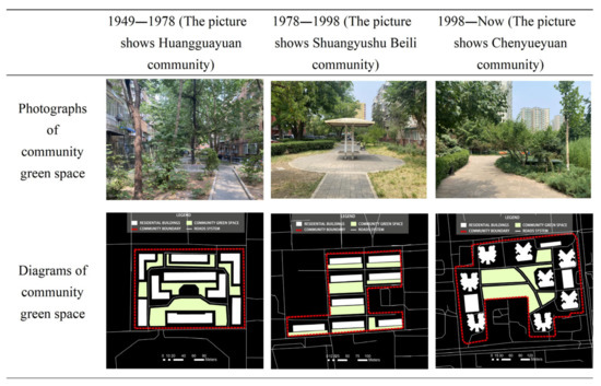
Figure 1.
Diagrams and photographs of typical community green space in each time stages.
3. Methodology
3.1. Case Selection and Data Sources
Housing policies and design specifications can pose a significant impact on the main urban area [33,34,35], so the study selected six main urban districts of Beijing as the study area, which are delineated according to the ring roads and street boundaries (Figure 2). Among the selected districts, Xicheng District and Dongcheng District are located within the 2 ring road and are the political-administrative districts of Beijing. Chaoyang District and Haidian District are mainly located within the 2–5 ring roads and carry Beijing’s financial and educational functions, respectively. Fengtai District and Shijingshan District are located in the western and southern suburbs of the city, respectively, carrying a large residential population. It should be emphasized that within the second ring road is the Historic Landscape Preservation Area [36], and there are special community types such as courtyards and single-family dormitories [37] that may affect the regional measurement results, so the area within the second ring road is excluded.
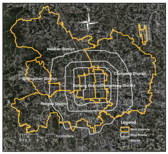
Figure 2.
Overview of the research area.
The data are of two categories: (1) urban-scale data, including the Shapefile data of main urban districts, ring roads, and 141 streets in the study area that were directly obtained from the OSM website [38]; and (2) community-scale data, including 3142 community boundary Shapefile data, 24,341 residential building AOI (Area of interest) data, and 20,109 green space AOI data in the study area, among which the community boundary data were obtained from the OSM website; residential building data were provided by the National Tibetan Plateau Data Center [39], and green space data were drawn from the Google Satellite Map [40].
3.2. Study Features and Measurement Methods
3.2.1. Measurement Methods of Service Efficiency
To accurately measure the service efficiency, the Regional Statistic method with low accuracy was excluded. In the Gravity Model method, the Gaussian-based 2-Step Floating Catchment Area (hereafter 2SFCA) method, which is widely applied in urban-scale green space studies, was selected. Since residents’ movement within the community is mainly via walking and the measurement results of spatial and temporal distance costs are similar, the Shortest Time Distance method was selected. The operation processes of the two methods were as follows: (1) the 2SFCA method: the method was proposed by Radke [41], and then Luo assigned a relative distance-based attenuation weight to it [42]. The mechanism of the method is shown in Figure 3, and the operation steps were as follows:
where is the scale of green space supply, measured by metric area, and is the search radius, measured in 150 m based on residents’ walking preference for community green space [43]. The demand point k in this study is the residential buildings in the communities where the green space is connected, and is the number of residents in each residential building. is the walking distance between the supply point and the demand point. is the Gaussian coefficient. is the sum of the supply intensity for each supply point within the search radius , with as the attenuation weight. The service efficiency level of community green space is reflected by the mean value of for the community. In this study, the measurement of 2SFCA was conducted through the geopandas module of Python to improve the efficiency of the calculation.
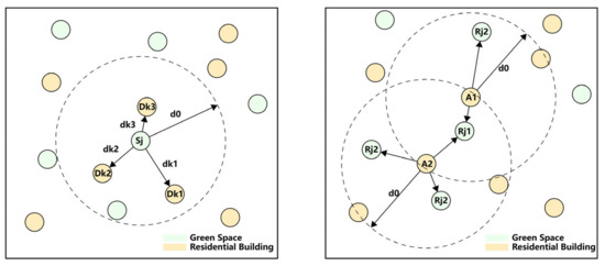
Figure 3.
The mechanism of 2SFCA method.
(2) Shortest Time Distance method: The method measures the shortest time cost taken by residents to reach the neighboring green space. In this study, the start point is each residential building in the case communities, and the endpoint is each green space in the corresponding community. The data from the OSM is difficult for ensuring the accuracy of the community road network and coordinating the actual road conditions in different study areas, while the Baidu Map API [44] provided us with a more accurate way: By entering the coordinates of the start and end points in the URL of the API, the walking time cost based on the big data of the map can be returned, and the shortest time distance can be filtered to enhance the accuracy and improve the efficiency of the calculation. The operation has three steps: 1. obtain the coordinates of each residential building and green space in the case communities by ArcMap; 2. take the residential buildings in each community as the start points and the green spaces as the endpoints to request the Baidu Map API to obtain the walking time costs between them; and 3. apply the smallest order in Python to filter the shortest time distance from the residential building to the neighboring green space. The service efficiency level of community green space is reflected by the mean value of the shortest time distance of the selected community. The mechanism of the method is shown in Figure 4. In this study, the processing of geographic data was conducted in the Arcmap, and the acquisition of the Shortest Time Distance values is achieved through the requests module of Python.
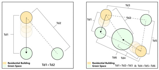
Figure 4.
The mechanism of the Shortest Time Distance method.
3.2.2. Measurement Methods of the Distribution Characteristics
Since there are few studies on the distribution characteristics of community green spaces, this part of the study had two steps: 1. preliminary identifying the distribution characteristics of community green spaces, and 2. proposing and applying a more effective quantitative measurement method based on the identification conclusion. These distribution characteristics are revealed through a process from identification to application.
Before the measurement, the Greening rates of the selected cases were conducted and classified by the built year ranges and urban ring road ranges to assess the impact of the area proportion indicator on the study, and the results are shown in Table 1 and Figure 5.

Table 1.
Spatial-temporal distribution of Greening rates.
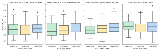
Figure 5.
Spatial-temporal distribution of Greening rates.
As shown in Table 2, the distribution of Greening rates varied little across urban locations and built year ranges. Except for the slightly higher values outside the 5-ring road during 1949–1978 and 1978–1998, the values in other conditions remained around 30%. Therefore, the study could exclude the interference of the area proportion factor in the measurement results and focus on the spatial-temporal pattern changes of the graphical distribution characteristics of community green spaces.
Table 2.
Spearman’s rank correlation coefficients between locations and built years.
To identify these graphical characteristics, Dou Q. inferred that there was an evolutionary pattern of green space from ‘courtyard’ type distribution among residential buildings to ‘centralized’ type distribution in the center of the community as the years progressed [45] (consistent with Table 1). The ‘courtyard’ type distribution indicates that the green spaces are located beside residential buildings and the time costs for residents to reach the nearest green space are evenly distributed, while the ‘centralized’ type distribution indicates that the time costs are unevenly distributed. Therefore, the identification step was conducted based on the orderliness degree of the shortest time distance distribution, and the method of Time Distance Entropy was introduced, which was calculated as follows:
Assuming that there were several residential buildings in the target community, all shortest time distances between residential buildings and adjacent green areas were divided into five sub-ranges, which represented 5 levels from ‘short’ to ‘long’, and then the numbers of residential buildings falling into each sub-range were counted, which were –. Finally, the time distance entropy of the target community was operated by the following equation:
The value of can reflect the orderliness degree of the shortest time distance distribution [46]; the higher the value, the smaller the correlation between the location of green spaces and residential buildings, and vice versa. The results of the Time Distance Entropy method can initially identify the ‘centralized’ and ‘courtyard’ type distributions.
It should be noted that this method can only initially identify the degree of ‘attachment/detachment’ of community green spaces to residential buildings but cannot characterize their graphical distribution at the planning level, so an accurate measurement of their spatial graphical distribution pattern will be proposed later in the article regarding the identification results. In this study, the measurement of the Time Entropy value was conducted through the geopandas module of Python.
3.2.3. Spatial-Temporal Dimension Model
The temporal dimension model is formed by classification according to the built-year ranges of the case communities. After the founding of the People’s Republic of China (PRC), the development of communities could be divided into the Danwei Compound phase from 1949 to 1978 [47], the Reformed Housing phase from 1978 to 1998, and the Commodity Housing phase from 1998 to the present [48]; therefore, the case communities were classified according to the three phases in the temporal dimension. The spatial dimension model is formed by classification according to the ring roads of Beijing; according to the spatial structure of Beijing, the case communities are classified into four categories: the 2–3 ring road, the 3–4 ring road, the 4–5 ring road, and those outside of the 5-ring road [49]. To visualize the spatial-temporal patterns of the measurement indicators, the measurement values of each indicator were divided by natural breaks into five levels (level 1–level 5) from small to large, then the case communities were divided based on the temporal dimension model, and finally, the percentage of the green spaces in different levels of communities of the spatial dimension model was calculated, which was displayed in a classification bar chart; meanwhile, the numbers of communities in each spatial range were also plotted as a reference.
To avoid the influence of excessive correlation between the two dimensions on the experimental results, Spearman’s rank correlation coefficients between the location of each case community and its built year under different temporal ranges were calculated, and the results are shown in Table 2. Most of the coefficients in the table are lower than 0.5, except for 1949–1978, where the coefficient is merely slightly larger than 0.5, indicating that there are no excessive correlations between the two and ensuring the value of conducting the study in both dimensions.
Supported by the above research methodology and data, the research framework of this paper is shown in Figure 6.
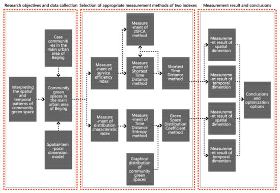
Figure 6.
The research framework of the paper.
4. Results
4.1. Spatial-Temporal Patterns of Service Efficiency
4.1.1. Service Efficiency Measurement Based on the 2SFCA Method
As per the research plan, the mean values of for each community were measured and presented through the spatial-temporal classification model (Table 3, Figure 7 and Figure 8). From the measurement results, it could be seen that:
Table 3.
Specific measurement results of the 2SFCA method.
Figure 7.
Measurement results of the 2SFCA method.
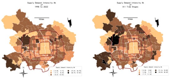
Figure 8.
The spatial-temporal patterns of the 2SFCA method.
(1) During 1949–1978, there were no communities with green space service efficiency of level 4 and level 5. The level 3 communities all appeared within the 2–3 ring road, accounting for 50.4% of the total. Level 2 communities were mainly found in the two ranges of the 2–4 ring road (accounting for 22.9% and 42.7%, respectively) and were not found in the 4–5 ring road. The proportions of level 1 communities in the 2–5 ring roads showed a significant upward trend with the outward expansion of the ring roads (accounting for 26.8%, 57.3%, and 100%, respectively). It should be noted that the number of communities outside the 5-ring road is very small (around 25, and slightly fluctuates with the drop of null value) in this period, and the randomness of the measurement results was accordingly significant, so the discussion outside the 5-ring road of this period was excluded. All the following operate like this.
(2) During 1978–1998, level 5 communities did not appear, and level 4 communities were evenly distributed in the two ranges of the 3–5 ring road (accounting for 39.8% and 39.6%, respectively) and were 18.3% outside the 5-ring road. Level 3 communities all appeared outside the 5-ring road (57.3%). The proportions of level 1 communities decreased with the outward expansion of the ring roads, and level 2 communities did not present an obvious distribution pattern.
(3) After 1998, level 5 communities emerged, and similar to level 4 communities, were all located in the 4–5 ring road (the proportions were 33.3% and 35.7%). Level 3 communities existed only outside the 3-ring road, with higher proportions in the 3–4 ring road and outside the 5-ring road (accounting for 41.5% and 32.4%, respectively), and with a lower proportion (10.6%) in the 4–5 ring road. The level 1 and level 2 communities took the 4–5 ring road as a watershed, decreasing in their internal ranges with the outward expansion (69.1% and 30.9% to 9.4% and 11.1%, respectively) and rebounding to 32.2% and 35.4%, respectively, in the external ranges.
Generally, there is an obvious ‘unipolar’ feature in the measurement by the 2SFCA method, i.e., communities with one single service efficiency level are concentrated in a narrow number of spatial ranges, leading to limitations in the division of service efficiency levels in other ranges, and even creating a situation where only one level exists in a certain range, making the method unable to comprehensively describe the spatial-temporal patterns of service efficiency on the community scale.
However, the above situation can be explained by the mechanism of the 2SFCA method. In the case communities, the neighboring building distance is around 20 m, while the preferred walking distance of residents is around 150 m. Therefore, different search areas may contain a large number of duplicate green spaces that the measurement results do not present significant differences within the same community, and hence the diversity of values is greatly reduced. In addition, communities of the same type produce approximate measure results and exhibit convergent measure values in the same range, resulting in the above situation.
4.1.2. Service Efficiency Measurement Based on the Shortest Time Distance Method
As per the research plan, the mean values of the shortest time distance for each community were measured and presented through the spatial-temporal classification model (Table 4, Figure 9 and Figure 10). From the measurement results, it could be seen that:
Table 4.
Specific measurement results of the Shortest Time Distance method.
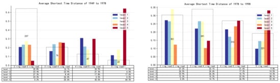
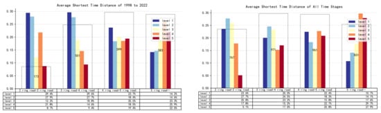
Figure 9.
Measurement results of the Shortest Time Distance method.
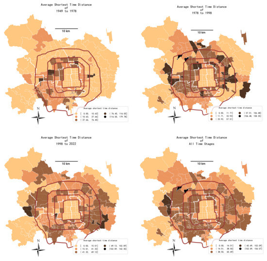
Figure 10.
The spatial-temporal patterns of the Shortest Time Distance method.
(1) During 1949–1978, level 1 and level 2 communities accounted for about 20.0% of the total number of the 2–5 ring road. Level 3 communities were evenly distributed in the other ranges (about 20.0%) except for a relatively small proportion in the 3–4 ring road (8.4%). All level 4 communities were evenly distributed in the ranges of the 2–4 ring road, accounting for 23.3% and 26.0%, respectively. Level 5 communities presented an increasing trend with the outward expansion of the ring roads (accounting for 5.2%, 25.6%, 30.0%, and 64.3%, respectively).
(2) During 1978–1998, the proportions of level 1 and level 2 communities declined with the outward expansion of the ring roads (27.2% and 26.5% to 9.8% and 14.5%, respectively). The proportion of level 3 communities was divided by the 4–5 ring road, decreasing with the outward expansion in the interior (33.9% to 10.7% from 2–3 ring to 4–5 ring) and rebounding to 14.3% in the exterior of the 5 ring road, while the proportions of level 4 and level 5 communities increased significantly with the outward expansion (12.3% and 0.0% to 28.1% and 33.2%, respectively).
(3) After 1998, the proportions of each level community showed an outward-shifting trend in the bar chart, with level 4 and level 5 communities sharing a similar proportion of each range as in 1978–1998 and level 3 communities showing an increasing trend (12.2% to 23.3%) with the outward expansion of the ring roads. Level 1 and level 2 communities had a proportion of around 30.0% in both ranges of the 2–4 ring road and then declined to about 14.0% with the outward expansion.
Generally, the Shortest Time Distance method provides an accurate and comprehensive measurement of the service efficiency of community green spaces; in the spatial dimension, the service efficiency of community green spaces decreases with the outward expansion of the ring roads (the shortest time distance is inversely proportional to service efficiency). In the temporal dimension, the community green spaces gradually establish standardized design strategies associated with their urban locations and, with the 4–5 ring road as a watershed, the service efficiency of the interior ranges is distributed in ascending order, while that of the exterior range is distributed in descending order. In addition, the proportions of high-level communities also increase over time.
Generally, the spatial-temporal patterns of the community green spaces’ service efficiency provide an insight into the community paradigm transformation of Beijing’s main urban area. In the early years of the People’s Republic of China, due to the limitations of the economic level and lack of construction experience, communities were funded by the government and distributed ‘for free or at low cost’ [50]. The green spaces were located directly in the open spaces next to the residences based on the principle of proximity to activities, making them unconstrained in the master plan and providing a desirable service efficiency. Later, with the implementation of the Reform and Opening Policy and Housing Commercialization Policy, communities began to exhibit commercialized attributes and serve as profit-oriented [51]. Real estate developers established standardized planning paradigms for the communities according to their urban locations to attract customers, which also made the community green spaces obey strict planning patterns; this is when the service efficiency decreased, and green spaces showed a standardized ascending or descending feature according to their urban locations.
4.2. Spatial-Temporal Patterns of Distribution Characteristics
4.2.1. Distribution Characteristic Identification Based on the 2SFCA Method
As per the research plan, the mean values of time distance entropy for each community were measured and presented through the spatial-temporal classification model (Table 5, Figure 11 and Figure 12). From the measurement results, it could be seen that:
Table 5.
Specific measurement results of the Time Distance Entropy method.
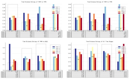
Figure 11.
Measurement results of the Time Distance Entropy method.
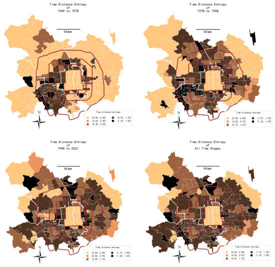
Figure 12.
The spatial-temporal patterns of the Time Distance Entropy method.
(1) During 1949–1978, the proportions of level 5 communities were similar across the ranges of the 2–5 ring road, accounting for 19.0%, 16.9%, and 19.2%, respectively, from the inner to outer rings. Level 4 communities were evenly distributed across the two ranges of 2–4 ring roads, with proportions of 22.3% and 25.5%, respectively, then decreasing to 10.0% in the 4–5 ring road. The proportions of level 3 communities decreased with the outward expansion of rings (23.1% to 8.7%), and the proportions of level 1 and level 2 communities increased in the same condition (19.4% and 16.2% to 25.8% and 36.4%, respectively).
(2) During 1978–1998, the overall values were evenly distributed across the 2–5 ring road, and the proportions of level 5 communities declined within the 5-ring road and rebounded outside the 5-ring road (21.9%, 19.0%, 15.5%, and 30.4% from the inner to outer rings). The proportions of level 2–level 4 communities were evenly distributed within the 2–5 ring road but decreased significantly outside the 5-ring road. The proportions of level 1 communities remained around 19.0% within the 2–4 ring road and 22.0% outside the 4 ring road, showing a slightly increasing trend.
(3) After 1998, the 2–3 ring road only accounted for less than 20.0% of the communities on most levels, except for the very large proportion of level 1 communities (46.7%). In other ranges, level 1 communities were all distributed in the 3–5 ring road, and the value increased slightly (21.5% to 25.9%) with the outward expansion of the ring roads. The number of level 2–level 5 communities mostly floated around 20.0%, among which the values of level 3-level 5 communities have an overall increasing trend with the outward expansion, while the proportions of other level communities remained stable.
The above results allow a preliminary identification of the distribution characteristics of community green spaces. In the spatial dimension, the time distance entropy values show a homogeneous distribution in each range, with the 5-ring road as the watershed. The internal ranges were mostly level 1–level 2 communities, mainly showing a ‘courtyard’ type distribution, while the external ranges were mostly level 4–level 5 communities, mainly showing a ‘concentrated’ type distribution. In the temporal dimension, the proportions of high-level communities increased through time, indicating that communities tend to adopt a ‘centralized’ type distribution of green space rather than a ‘courtyard’ type as time progresses, and the locations of community construction also showed a slight tendency to move outward over time.
4.2.2. Proposal and Application of the Green Space Distribution Coefficient Method
The results of the Shortest Time Distance method show that residents tend to choose green space activities in close proximity, and the spatial-temporal pattern of Time Distance Entropy also initially reveals the transition of community green space distribution characteristics from a ‘courtyard’ type to a ‘centralized’ type, so this section will propose a more accurate and graphical evaluation method for green space distribution characteristics based on the above results and describe their spatial-temporal patterns in detail.
Figure 13 displays the spatial distribution diagram of community green space based on the results of the Shortest Time Distance method and the Time Distance Entropy method, showing public activity preferences of the ‘courtyard’ and ‘centralized’ type green space, respectively.
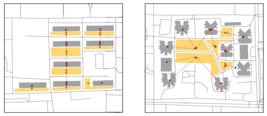
Figure 13.
The spatial distribution diagram of community green space.
According to Figure 5, the Greening rate did not vary significantly in the spatial and temporal dimensions, so the number of green spaces in the community was inversely proportional to the average area of each green space in the community, and the number of ‘courtyard’ type green spaces in the community was much larger than that of ‘centralized’ green spaces. It is further inferred that if the number of green spaces in a community is large and the average distance between them and the neighboring residences is small, they tend to show a ‘courtyard’ type distribution and, vice versa, a ‘concentrated’ type distribution. Based on this conclusion, this paper proposes the Green Space Distribution Coefficient Fg to measure this graphical feature, and its operation process is as follows:
In the above equation, represents the number of green spaces in the community, , ... represent the shortest time distance between each green space and the neighboring residential buildings, and is the mean value of the shortest distances. The larger the , the more green spaces in the community tend to be distributed in a ‘courtyard’ type distribution and, vice versa, in a ‘centralized’ type distribution. According to this method, the Fg of each community were calculated and presented by the spatial-temporal classification model (Table 6, Figure 14 and Figure 15). In this study, the measurement of the Green Space Distribution Coefficient value was conducted through the geopandas module of Python. From the measurement results, it could be seen that:
Table 6.
Specific measurement results of the Green Space Distribution Coefficient method.
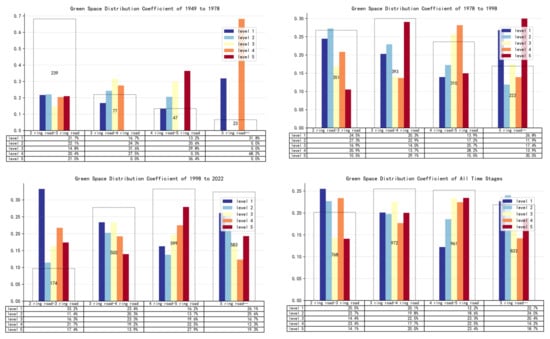
Figure 14.
Measurement results of the Green Space Distribution Coefficient method.
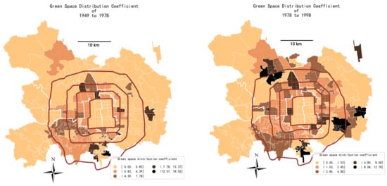
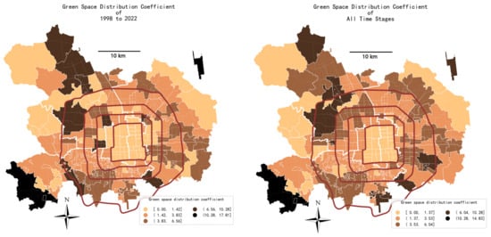
Figure 15.
The spatial-temporal pattern of the Green Space Distribution Coefficient method.
(1) During 1949–1978, level 1–level 5 communities were concentrated in the 2–3 ring road. Most of them had no significant difference in the proportions of communities in each level (about 20.0%), except for a slightly smaller percentage of level 3 communities (14.8%). In the other rings, the sums of level 1–level 2 communities and level 4–level 5 communities were close to each other, indicating that the green spaces in this stage presented the distribution characteristics of both ‘courtyard’ type and ‘centralized’ type, which is defined as a ‘mixed’ type distribution characteristic in this paper.
(2) During 1978–1998, except for the proportions of level 1–level 2 communities in the 2–3 ring road (accounting for 24.5% and 27.3% respectively), which held larger proportions than level 4–level 5 (accounting for 20.9% and 10.5% respectively), the proportions of high-level communities in all other ranges was larger than that of low-level communities; in particular, the proportions of level 4–level 5 communities were significantly larger than those of level 1–level 2 communities in the two ranges of the 3–5 ring road with a large community amount, indicating that the community green space outside of the 3-ring road had already been extensively designed in a ‘courtyard’ type distribution.
(3) After 1998, community green spaces within the 4–5 ring road were mainly distributed in the ‘courtyard’ type, while the community green spaces of other ranges were mainly distributed in a ‘centralized’ type. It is speculated that because Beijing’s universities, research institutions, urban parks, and Olympic venues are mainly concentrated in the 4–5 ring road, the communities within the range have more staff dormitories, student dormitories, or family apartments, and therefore maintain a ‘welfare’ attribute [52], while the rest of the ranges are developed for ‘commercialization’ purposes, and ‘centralized’ type green spaces are widely applied in community planning to meet the aesthetic and efficient spatial layout.
The results of the above measures provide an in-depth description of the spatial-temporal patterns of community green space distribution characteristics. In the spatial dimension, unlike the time distance entropy, the community green spaces between the 4–5 ring road maintain a ‘courtyard’ type distribution, except for the green spaces of the other ranges, which show a ‘concentrated’ type distribution. In the temporal dimension, except for the distribution of community green spaces in the 4–5 ring road, which did not change significantly over time, the community green spaces in all other ranges showed a ‘mixed-courtyard-centralized’ evolutionary pattern. In general, the Green Space Distribution Coefficient method revealed the distribution characteristics of community green spaces more comprehensively, and the analysis results also presented a good fit with the spatial patterns in Table 1.
Generally, the spatial-temporal patterns of the distribution characteristics of community green spaces provide insight into the transformation of the residential cultures of Beijing’s communities. In the early years of the People’s Republic of China, communities were mostly in the form of ‘unit compounds’, and the planning paradigm was at the exploratory stage [53]. Although most of the green areas were arranged near residential buildings, there were still a few ‘centralized’ green areas that did not obey this feature, thus showing a ‘mixed’ type distribution. Later, due to economic resource constraints, community green spaces began to follow a strict ‘courtyard’ type distribution, efficiently serving adjacent residential buildings while also providing residents with private, small-scale places to interact and form a close neighborhood relationship. This relationship has been disrupted by the commodification of housing, which has led to more ‘centralized’ green space in subsequent neighborhoods, which, while more open, denies a sense of security and privacy to immediate neighbors and reduces the tendency for more distant residents to engage in public activities. Furthermore, community green spaces in the inner ring road ranges of the city are generally the ‘courtyard’ types of distribution, while those in the outer ranges are generally the ‘concentrated’ types of distribution, further suggesting that policies tend to constrain the main districts of the city more strictly, while communities in the outer ranges are generally oriented to maximize benefits.
4.3. Discussion
Through the measurement results, the study classifies the communities in the main urban area of Beijing according to the spatial-temporal dimension model and tries to provide practical suggestions for optimizing the service quality of community green spaces. As shown in Table 2, since there is no significant correlation between the temporal and spatial dimensions, the optimization suggestions will be presented in the above two dimensions, respectively:
(i) In the temporal dimension, green spaces in the communities built between 1949 and 1978 are mainly of the ‘mixed’ type distribution, carrying private communications of close neighbors and ensuring community-wide public activities through local large-scale green spaces. However, their service efficiency levels are evenly distributed and can still be improved, so the distance between local ‘courtyard’ type green spaces and residential buildings should be reduced, while the master plan for community green spaces should be maintained. Green spaces in the communities built between 1978 and 1998 are mainly of the ‘courtyard’ type distribution with high service efficiency, but they lacked community-scale gathering places, so the ‘courtyard’ type green spaces in the center of the community could be expanded or the ends of the closed ‘pocket-like’ roads could be transformed into ‘centralize’ type green spaces. In addition, the form of green spaces can be optimized to be more attractive. Green spaces in the communities built since 1998 are mainly of the ‘centralized’ type distribution, lacking places for communication between close neighbors, and the distribution of service efficiency levels is extremely uneven, so it is necessary to add ‘courtyard’ type green spaces near residential buildings, while ‘centralized’ type green spaces can also be partially divided into ‘courtyard’ type green spaces.
(ii) In the spatial dimension, with the 4–5 ring road as a watershed, community green spaces present great service efficiency in their interior but are more neglectful of service efficiency in the exterior, so it is needed to curtail the distance between green spaces and residential buildings in communities outside the 5 ring road to make the community green spaces more accessible. In addition, most of the communities outside the 4–5 ring road are of the ‘centralize’ type distribution, so it is needed to increase the amount of ‘courtyard’ type green spaces to stimulate intimate communications between close neighbors. Community green spaces of the 4–5 ring road mainly preserve the ‘courtyard’ type distribution, so in the optimization process, some local ‘courtyard’ type green spaces can be combined into a ‘centralized’ green space to carry the community-wide public activities. Besides, the distribution types of community green spaces within the 4 ring road need to be specifically classified according to the Green Space Distribution Coefficient and then targeted for optimization.
In addition, the measurement results of the Shortest Time Distance and the Green Space Distribution Coefficient can be applied as a guide to optimize the service quality of community green spaces in specific cases and to support the development of relevant policies.
5. Conclusions
This section may be divided into subheadings. It should provide a concise and precise description of the experimental results, their interpretation, as well as the experimental conclusions that can be drawn.
The above research process allows for the following responses to the research questions posed in this paper:
1. The Shortest Time Distance method can effectively measure the service efficiency of green spaces on the community scale, while the 2FSCA method is less effective. As the results of the Shortest Time Distance method are more concise and intuitive, they are closer to the public activity preferences of residents on the community scale, and their accuracy can be guaranteed with the assistance of Baidu Map API, while the area search property of the 2SFCA method affects the delineation of its measurement levels, making it difficult to describe the service efficiency of the community green spaces comprehensively.
2. According to Time Distance Entropy measurement results, this paper proposes a Green Space Distribution Coefficient method based on the ‘courtyard’ and ‘centralized’ type distributions of community green spaces. Unlike Time Distance Entropy, the calculation of the Green Space Distribution Coefficient not only contains the locational relationships between green spaces and neighboring residential buildings but also includes the spatial graphical elements of green space in the community, which can describe the distribution characteristics more comprehensively and accurately. It also analyzes the ‘mixed’ type distribution characteristics that have not been found in the existing studies.
3. The results of the Shortest Time Distance method and the Green Space Distribution Coefficient method allow the following conclusions of the spatial-temporal patterns of the service efficiency and distribution characteristics of the community green spaces:
(i) Based on the temporal pattern of service efficiency, green spaces follow a trend of becoming standardized and this indicator spontaneously decreases due to excessive obedience to graphical constraints during the transformation of communities from ‘welfare’ to ‘commercial’ attributes. Based on the spatial pattern, the service efficiency of community green spaces tends to decrease with the outward expansion of the ring roads, indicating that communities tend to provide desirable green space service quality in the inner ranges while neglecting this indicator in the outer ranges.
(ii) Based on the temporal pattern of distribution characteristics, community green space has undergone the evolutionary process of ‘mixed type-courtyard type-centralized type,’ indicating that it actually underwent an ‘exploration process’ in the early stage of the People’s Republic of China, and adopted ‘courtyard’ type distribution afterwards to cope with the poor economic level of the reform housing phase, and subsequently adopted ‘centralized’ distribution to comply with the principle of profit maximization in the commodity housing phase. Based on the spatial patterns, except for the community green space in the 4–5 ring road, which has always maintained a ‘courtyard’ type distribution, those in the interior ranges have changed from ‘courtyard’ to ‘centralized’ type with the commercialization of housing, while that in the exterior range has always maintained a ‘centralized’ type distribution.
4. Taking the spatial-temporal patterns of the service efficiency and distribution characteristics of community green space as a perspective, the following transformation process of Beijing’s community paradigms and residential cultures can be interpreted:
(i) According to the spatial-temporal patterns of the service efficiency of green spaces, the community paradigms generally show an orientation transformation from ‘humanistic-oriented’ to ‘benefit-oriented’ with the passage of the built years and the outward expansion of construction sites. From the temporal dimension, the early community green spaces lacked graphical constraints but guaranteed the convenience of public activities, while the later community green spaces had a standardized design paradigm but neglected the satisfaction of convenience due to the excessive pursuit of attraction and profit factors. From the spatial dimension, community green spaces in the inner ring road ranges show high service efficiency and provide good quality public activities, while the outer ranges neglect the quality of public activities in order to guarantee lower design costs and shorter construction cycles.
(ii) According to the spatial-temporal patterns of the distribution characteristic of green spaces, the residential cultures of the community change from ‘closeness’ to ‘detachment’ with the passage of the built years and the outward expansion of construction sites. From the temporal dimension, the early ‘courtyard’ type community green spaces provided small-scale places for neighborhood interaction, while the ‘centralized’ type distribution of community green spaces in later years replaced such places. From the spatial dimension, except for the 4–5 ring road community green spaces, which always maintain the ‘courtyard’ distribution, the community green spaces in the inner ranges are initially of ‘courtyard’ type and ‘mixed’ type distribution characteristics in the early stage, which establish a close neighborhood network. In the later stages, however, they are affected by the housing commercialization policy and show the ‘centralized’ type distribution characteristic, which destroys this close network, while the community green spaces in the outer ranges mostly show the ‘centralized’ type distribution characteristics, and the neighborhood relationship is always more distant.
Based on the above conclusions, this paper attempts to propose the following optimization options for community green spaces in Beijing: For communities built in the early years and located in the inner ranges (within the 4 ring road), the parts of the ‘courtyard’ type and ‘mixed’ type green spaces that have good service efficiency should be preserved and optimized to maintain the ‘humanistic’ and ‘closeness’ characteristics of the community, while ‘centralized’ type green spaces should be added in places to optimize the community landscape and ensure public activities on the community scale. For the communities built later and located in the outer ranges (outside the 5-ring road), there is a need to increase the proportion of ‘courtyard’ type green space, while reducing the relative distance between green spaces and neighboring residential buildings, to provide better service efficiency and create a close-knit neighborhood environment. For communities within the 4–5 ring road, it is necessary to develop appropriate renewal strategies for optimization based on the specific community attributes (‘welfare’ or ‘commercial’) and evaluation results. The methods evaluated in this paper can also provide quantitative guidance on its design strategies and optimization interventions. In addition, this paper also expects to inspire more attention and discussion on community green space with the support of the above conclusions.
Author Contributions
Conceptualization, Xiaoyi Zu, Chen Gao, Zhixian Li and Yi Wang; methodology, Xiaoyi Zu; software, Xiaoyi Zu; validation, Zhixian Li and Chen Gao; formal analysis, Xiaoyi Zu; investigation, Xiaoyi Zu; resources, Zhixian Li and Chen Gao; data curation, Xiaoyi Zu; writing—original draft preparation, Xiaoyi Zu, Zhixian Li and Chen Gao; writing—review and editing, Xiaoyi Zu, Zhixian Li and Chen Gao; visualization, Xiaoyi Zu; Supervision, Yi Wang; and project administration, Zhixian Li, Chen Gao and Yi Wang. All authors have read and agreed to the published version of the manuscript.
Funding
This research received no external funding.
Data Availability Statement
Openstreetmap.com (accessed on 15 June 2021) for the data of urban-scale and community boundary; data.tpdc.ac.cn (accessed on 25 June 2022) for the data of residential building; and google.com (accessed on 20 July 2022) for the data of green space.
Acknowledgments
The open access publication of this article has been financially supported by the Leibniz Institute for Research on Society and Space (IRS). As a member of the Leibniz-Association, the IRS is funded by the Federal Republic and the Federal States of Germany.
Conflicts of Interest
The authors declare no conflict of interest.
References
- Chiesura, A. The Role of Urban Parks for the Sustainable City. Landsc. Urban Plan. 2004, 68, 129–138. [Google Scholar] [CrossRef]
- Bedimo-Rung, A.L.; Mowen, A.J.; Cohen, D.A. The Significance of Parks to Physical Activity and Public Health. Am. J. Prev. Med. 2005, 28, 159–168. [Google Scholar] [CrossRef] [PubMed]
- Wang, J. Towards a Better Understanding of Green Infrastructure—A Critical Review. Ecol. Indic. 2018, 85, 758–772. [Google Scholar]
- Lee, A.C.K.; Maheswaran, R. The Health Benefits of Urban Green Spaces: A Review of the Evidence. J. Public Health 2011, 33, 212–222. [Google Scholar] [CrossRef]
- Wiseman, L.M.; Kelly, J.F.; McGough, R.J. Exact and Approximate Analytical Time-Domain Green’s Functions for Space-Fractional Wave Equations. J. Acoust. Soc. Am. 2019, 146, 1150–1163. [Google Scholar] [CrossRef] [PubMed]
- La Rosa, D. Accessibility to Greenspaces: GIS Based Indicators for Sustainable Planning in a Dense Urban Context. Ecol. Indic. 2014, 42, 122–134. [Google Scholar] [CrossRef]
- Xu, Z.; Zhang, Z.; Li, C. Exploring Urban Green Spaces in China: Spatial Patterns, Driving Factors and Policy Implications. Land Use Policy 2019, 89, 104249. [Google Scholar] [CrossRef]
- Kong, F.; Yin, H.; Nakagoshi, N.; Zong, Y. Urban Green Space Network Development for Biodiversity Conservation: Identification Based on Graph Theory and Gravity Modeling. Landsc. Urban Plan. 2010, 95, 16–27. [Google Scholar] [CrossRef]
- Zhao, Y.; Zhang, G.; Zhao, H. Spatial Network Structures of Urban Agglomeration Based on the Improved Gravity Model: A Case Study in China’s Two Urban Agglomerations. Complexity 2021, 2021, 6651444. [Google Scholar] [CrossRef]
- Jung, W.-S.; Wang, F.; Stanley, H.E. Gravity Model in the Korean Highway. EPL 2008, 81, 48005. [Google Scholar] [CrossRef]
- Loughran, K. Urban Parks and Urban Problems: An Historical Perspective on Green Space Development as a Cultural Fix. Urban Stud. 2020, 57, 2321–2338. [Google Scholar] [CrossRef]
- Tang, H.; Liu, W.; Yun, W. Spatiotemporal Dynamics of Green Spaces in the Beijing–Tianjin–Hebei Region in the Past 20 Years. Sustainability 2018, 10, 2949. [Google Scholar] [CrossRef]
- Sun, Y.; Li, Y.; Gao, J.; Yan, Y. Spatial and Temporal Patterns of Urban Land Use Structure in Small Towns in China. Land 2022, 11, 1262. [Google Scholar] [CrossRef]
- Borana, S.L.; Vaishnav, A.; Yadav, S.K.; Parihar, S.K. Urban Growth Assessment Using Remote Sensing, GIS and Shannon’s Entropy Model: A Case Study of Bhilwara City, Rajasthan. In Proceedings of the 2020 3rd International Conference on Emerging Technologies in Computer Engineering: Machine Learning and Internet of Things (ICETCE), Jaipur, India, 7–8 February 2020; pp. 1–6. [Google Scholar] [CrossRef]
- Lv, F.; Yan, Y.L. Health-Oriented Community Slow Greenway’s Planning and Design. AMR 2013, 671–674, 2371–2375. [Google Scholar] [CrossRef]
- Sallis, J.F.; Cervero, R.B.; Ascher, W.; Henderson, K.A.; Kraft, M.K.; Kerr, J. An Ecological Approach to Creating Active Living Communities. Annu. Rev. Public Health 2006, 27, 297–322. [Google Scholar] [CrossRef] [PubMed]
- Bergeron, K.; Lévesque, L. Designing Active Communities: A Coordinated Action Framework for Planners and Public Health Professionals. J. Phys. Act. Health 2014, 11, 1041–1051. [Google Scholar] [CrossRef]
- Lang, W. A New Style of Urbanization in China: Transformation of Urban Rural Communities. Habitat Int. 2016, 55, 1–9. [Google Scholar] [CrossRef]
- He, J.; Yi, H.; Liu, J. Urban Green Space Recreational Service Assessment and Management: A Conceptual Model Based on the Service Generation Process. Ecol. Econ. 2016, 124, 59–68. [Google Scholar] [CrossRef]
- Grunewald, K.; Richter, B.; Meinel, G.; Herold, H.; Syrbe, R.-U. Proposal of Indicators Regarding the Provision and Accessibility of Green Spaces for Assessing the Ecosystem Service “Recreation in the City” in Germany. Int. J. Biodivers. Sci. Ecosyst. Serv. Manag. 2017, 13, 26–39. [Google Scholar] [CrossRef]
- Luo, C.; Li, X. Assessment of Ecosystem Service Supply, Demand, and Balance of Urban Green Spaces in a Typical Mountainous City: A Case Study on Chongqing, China. Int. J. Environ. Res. Public Health 2021, 18, 11002. [Google Scholar] [CrossRef]
- Gretchen, D. Nature’s Services: Societal Dependence on Natural Ecosystems. Pac. Conserv. Biol. 2000, 6, 274. [Google Scholar] [CrossRef]
- Coombes, E.; Jones, A.P.; Hillsdon, M. The Relationship of Physical Activity and Overweight to Objectively Measured Green Space Accessibility and Use. Soc. Sci. 2010, 70, 816–822. [Google Scholar] [CrossRef]
- Yu, K.; Duan, W.; Li, D.; Peng, J. Evaluation Methods and Examples of Landscape Accessibility as a Functional Indicator of Urban Green Space Systems. Urban Plan 1999, 8, 7–10. [Google Scholar]
- Liu, C.; Li, X.; Han, D. Accessibility Analysis of Urban Parks: Method Sand Key Issues. Acta Ecol. Sin. 2010, 30, 5381–5390. [Google Scholar]
- Potestio, M.L.; Patel, A.B.; Powell, C.D.; McNeil, D.A.; Jacobson, R.D.; McLaren, L. Is There an Association between Spatial Access to Parks/Green Space and Childhood Overweight/Obesity in Calgary, Canada? Int. J. Behav. Nutr. Phys. Act. 2009, 6, 77. [Google Scholar] [CrossRef]
- Xing, L.; Liu, Y.; Liu, X. Measuring Spatial Disparity in Accessibility with a Multi-Mode Method Based on Park Green Spaces Classification in Wuhan, China. Appl. Geogr. 2018, 94, 251–261. [Google Scholar] [CrossRef]
- Coppel, G.; Wüstemann, H. The Impact of Urban Green Space on Health in Berlin, Germany: Empirical Findings and Implications for Urban Planning. Landsc. Urban Plan. 2017, 167, 410–418. [Google Scholar] [CrossRef]
- Olsen, L.M.; Dale, V.H.; Foster, T. Landscape Patterns as Indicators of Ecological Change at Fort Benning, Georgia, USA. Landsc. Urban Plan. 2007, 79, 137–149. [Google Scholar] [CrossRef]
- Comber, A.; Brunsdon, C.; Green, E. Using a GIS-Based Network Analysis to Determine Urban Greenspace Accessibility for Different Ethnic and Religious Groups. Landsc. Urban Plan. 2008, 86, 103–114. [Google Scholar] [CrossRef]
- Tang, Z.; Gu, S. An Evaluation of Social Performance in the Dist Ribution of Urban Parks in the Central City of Shang Hai: From Spatial Equity to Social Equity. Urban Plan. Forum 2015, 222, 48–56. [Google Scholar] [CrossRef]
- Zhang, Y.; Meng, J. Exploring the Renewal Strategy of Old Community Public Space Based on the Concept of “Sharing—The Example of Guizhou Xililong Community in Shanghai. Urban Dev. Stud. 2020, 8, 89–93. [Google Scholar]
- Marsal-Llacuna, M.-L. City Indicators on Social Sustainability as Standardization Technologies for Smarter (Citizen-Centered) Governance of Cities. Soc. Indic. Res. 2016, 128, 1193–1216. [Google Scholar] [CrossRef]
- Owens, A. How Do People-Based Housing Policies Affect People (and Place)? Hous. Policy Debate 2017, 27, 266–281. [Google Scholar] [CrossRef]
- Power, A. Social Inequality, Disadvantaged Neighbourhoods and Transport Deprivation: An Assessment of the Historical Influence of Housing Policies. J. Transp. Geogr. 2012, 21, 39–48. [Google Scholar] [CrossRef]
- Zhou, S.; Wu, L.; Yang, F.; Guo, J. The Relationship between Spatial Changes in Urban Entities and the Preservation of Historical Place Names—A Case Study of the Area within the Second Ring Road of Beijing. China Place Name 2007, 1, 66–67. [Google Scholar]
- Wang, Y. A Century of Change; The Urban Book Series; Springer International Publishing: Cham, Switzerland, 2016; ISBN 978-3-319-39632-3. [Google Scholar]
- OSM. Available online: https://www.openstreetmap.org/relation/912940 (accessed on 15 June 2020).
- The Residential Building AOI Data. Available online: http://data.tpdc.ac.cn (accessed on 25 June 2020).
- Google Earth. Available online: https://earth.google.com/web/ (accessed on 20 July 2020).
- Radke, J.; Mu, L. Spatial Decompositions, Modeling and Mapping Service Regions to Predict Access to Social Programs. Ann. GIS 2000, 6, 105–112. [Google Scholar] [CrossRef]
- Luo, W.; Wang, F. Measures of Spatial Accessibility to Health Care in a GIS Environment: Synthesis and a Case Study in the Chicago Region. Environ. Plan. B Plan. Des. 2003, 30, 865–884. [Google Scholar] [CrossRef]
- Wang, L.; Liu, R. The Small Is Big: The Development and Analysis of the Concept of Urban Small-Micro Public Spaces. New Archit. 2019, 3, 104–108. [Google Scholar]
- Baidu Map API. Available online: https://lbsyun.baidu.com/ (accessed on 1 June 2020).
- Dou, Q. A Space Syntax Investigation of The Changes in Residential District Planning and Design in Beijing. Archit. J. 2010, 1, 28–32. [Google Scholar]
- Li, M.; Ma, Y.; Sun, X.; Wang, J.; Dang, A. Application of Spatial and Temporal Entropy Based on Multi-Source Data for Measuring the Mix Degree of Urban Functions. City Plan. Rev. 2018, 42, 97–103. [Google Scholar]
- Zeng, X. Urbanisation and the New Urbanisation Road with Chinese Characteristics, 1st ed.; Wuhan University: Wuhan, China, 2020; ISBN 978-7-307-21677-8. [Google Scholar]
- Zu, X.; Gao, C. Evaluation and Optimization of Access Control Strategies for Neighborhood Residential Areas in the Post-Epidemic Era Based on Commercial Activation Purpose. Archicreation 2021, 6, 191–199. [Google Scholar]
- Tian, G.; Wu, J.; Yang, Z. Spatial Pattern of Urban Functions in the Beijing Metropolitan Region. Habitat Int. 2010, 34, 249–255. [Google Scholar] [CrossRef]
- Akiyama, C. Beijing Metropolitan Area. In Urban Development in Asia And Africa: Geospatial Analysis of Metropolises; Murayama, Y., Kamusoko, C., Yamashita, A., Estoque, R., Eds.; Springer: Berlin/Heidelberg, Germany, 2017; pp. 65–83. ISBN 2365-757X. [Google Scholar]
- Wu, Y.; Tian, L. The Impact of Residential Land Use Control on Housing Development: The Case of Beijing, China. Urban Stud. 2022, 29, 124–132. [Google Scholar]
- Yan, Y. Reflections on the Definition of Beijing Urban Area. Beijing Obs. 2004, 1, 30–32. [Google Scholar]
- Han, L.; Wang, B. Research on the Community Renewal of “Active Adaptation to the Elderly” in the Unit Compound. In Proceedings of ECSF 2021; Springer: Cham, Switzerland, 2022. [Google Scholar]


Publisher’s Note: MDPI stays neutral with regard to jurisdictional claims in published maps and institutional affiliations. |
© 2022 by the authors. Licensee MDPI, Basel, Switzerland. This article is an open access article distributed under the terms and conditions of the Creative Commons Attribution (CC BY) license (https://creativecommons.org/licenses/by/4.0/).