
The Use of Spatial Interpolation to Improve the Quality of Corn Silage Data in Case of Presence of Extreme or Missing Values


Abstract
:1. Introduction
- –
- Examine whether an interpolation method can improve field data quality by reducing the expected crop field variability, and to what extent this can be achieved.
- –
- Examine whether an interpolation method can effectively address the problems of extreme or missing values in data.
2. Materials and Methods
3. Results
4. Discussion
5. Conclusions
Author Contributions
Funding
Institutional Review Board Statement
Informed Consent Statement
Acknowledgments
Conflicts of Interest
References
- Kosmowski, F.; Chamberlin, J.; Ayalew, H.; Sida, T.; Abay, K.; Graufurd, P. How accurate are yield estimates from crop cuts? Evidence from smallholder maze farms in Ethiopia. Food Policy 2021, 102, 102122. [Google Scholar] [CrossRef] [PubMed]
- Wahab, I.; Jirstrom, M.; Hall, O. An Integrated Approach to Unravelling Smallholder Yield Levels: The Case of Small Family Farms, Eastern Region, Ghana. Agriculture 2020, 19, 206. [Google Scholar] [CrossRef]
- Wahab, I. In-season plot area loss and implications for yield estimation in smallholder rainfed farming systems at the village level in Sub-Saharan Africa. GeoJournal 2020, 85, 1553–1572. [Google Scholar] [CrossRef] [Green Version]
- Abay, K.A.; Abate, G.T.; Barrett, C.B.; Bernard, T. Correlated non-classical measurement errors, ‘Second best’ policy inference, and the inverse size-productivity relationship in agriculture. J. Dev. Econ. 2019, 139, 171–184. [Google Scholar] [CrossRef] [Green Version]
- Carletto, C.; Gourlay, S. A thing of the past? Household surveys in a rapidly evolving (agricultural) data landscape: Insights from the LSMS-ISA. Agric. Econ. 2019, 50 (Suppl. S1), 51–62. [Google Scholar] [CrossRef]
- Casley Dennis, J.; Kumar, K. The Collection, Analysis, and Use of Monitoring and Evaluation Data. In Third World Planning Review; Liverpool University Press: Liverpool, UK, 1988; p. 91. [Google Scholar] [CrossRef]
- Verma, V.; Marchant, T.; Scott, C. Evaluation of Crop-Cut Methods and Farmer Reports for Estimating Crop Production: Results of a Methodological Study in Five African Countries; Longacre Agricultural Development Centre Limited: London, UK, 1988; p. 75. [Google Scholar] [CrossRef]
- Lobell, D.B.; Azzari, G.; Burke, M.; Gourlay, S.; Jin, Z.; Kilic, T.; Murray, S. Eyes in the Sky, Boots on the Ground: Assessing Satellite- and Ground-Based Approaches to Crop Yield Measurement and Analysis. Am. J. Agric. Econ. 2020, 102, 202–219. [Google Scholar] [CrossRef]
- FAO—Food and Agriculture Organization of the United Nations. Methodology for Estimation of Crop Area and Crop Yield under Mixed and Continuous Cropping. In Publication Prepared in the Framework of the Global Strategy to Improve Agricultural and Rural Statistics; FAO: Rome, Italy, 2017. [Google Scholar]
- Piepho, H.P.; Mohring, J.; Williams, E.R. Why Randomize Agricultrural Experiments? J. Agron. Crop Sci. 2013, 199, 374–383. [Google Scholar] [CrossRef]
- Fermont, A.; Benson, T. Estimating Yield of Food Crops Grown by Smallholder Farmers: A Review in the Uganda Context; IFPRI Discuss Pap. 01097; IFPRI: Washington, DC, USA, 2011; pp. 1–57. [Google Scholar]
- Hagblad, L. Crop Cutting Versus Farmer Reports–Review of Swedish Findings. In Statistik Rapport 1998, 2; Statistics Sweden: Örebro, Sweden, 1988. [Google Scholar]
- Murphy, J.; Casley, D.J.; Curry, J.J. Farmers’ estimations as a source of production data. In World Bank Technical Paper 132; World Bank Publication: Washington, DC, USA, 1991. [Google Scholar]
- Liu, Q.; Feng, G.; Zheng, W.; Tian, J. Managing data quality of cooperative information systems: Model and algorithm. Expert Syst. Appl. 2022, 189, 116074. [Google Scholar] [CrossRef]
- Srinath, Y.; Vijayakumar, K.; Revathy, S.M.; Rangaraj, A.G.; Sheelarani, N.; Boopathi, K.; Balaraman, K. Automated Data Quality Mechanism and Analysis of Meteorological Data Obtained from Wind-Monitoring Stations of India. In Data Management, Analytics and Innovation; Lecture Notes on Data Engineering and Communications Technologies; Springer: Singapore, 2022; pp. 237–262. [Google Scholar]
- Taleb, I.; Serhani, M.A.; Bouhaddioui, C.; Dssouli, R. Big data quality framework: A holistic approach to continuous quality management. J. Big Data 2021, 8, 76. [Google Scholar] [CrossRef]
- Desiere, S.; Jolliffe, D. Land productivity and plot size: Is measurement error driving the inverse relationship? J. Dev. Econ. 2018, 130, 84–98. [Google Scholar] [CrossRef] [Green Version]
- Kim, T.; Ko, W.; Kim, J. Analysis and Impact Evaluation of Missing Data Imputation in Day-ahead PV Generation Forecasting. Appl. Sci. 2018, 9, 204. [Google Scholar] [CrossRef] [Green Version]
- Gomez, K.; Gomez, A. Statistical Procedures for Agricultural Research, 2nd ed.; John Wiley & Sons: New York, NY, USA, 1984; pp. 276–294. [Google Scholar]
- Steel, R.G.D.; Torrie, J.H.; Dickey, D.A. Principles and Procedures for Statistics: A Biometrical Approach, 3rd ed.; McGraw Hill: Boston, MA, USA, 1997; pp. 416–420. [Google Scholar]
- Li, T.; Hutfless, S.; Scharfstein, D.; Daniels, M.; Hogan, J.; Little, R.; Roy, J.; Law, A.; Diskersin, K. Standards in the Prevention and Handling of Missing Data for Patient Centered Outcomes Research—A Systematic Review and Expert Consensus. J. Clin. Epidemiol. 2014, 67, 15–32. [Google Scholar] [CrossRef] [PubMed] [Green Version]
- Webster, R.; Oliver, M.A. Geostatistics for Environmental Scientists, 2nd ed.; John Wiley & Sons Ltd.: West Sussex, UK, 2007. [Google Scholar]
- Wiens, D.P.; Zhou, Z. Robust estimators and designs for field experiments. J. Stat. Plan Inference 2008, 138, 93–104. [Google Scholar] [CrossRef]
- Cho, J.B.; Guinness, J.; Kharel, T.P.; Sunoj, S.; Kharel, D.; Oware, E.K.; van Aardt, J.; Ketterings, Q.M. Spatial estimation methods for mapping corn silage and grain yield monitor data. Precis. Agric. 2021, 22, 1501–1520. [Google Scholar] [CrossRef]
- Buttafuoco, G.; Castrignanò, A.; Cucci, G.; Lacolla, G.; Lucà, F. Geostatistical modelling of within-field soil and yield variability for management zones delineation: A case study in a durum wheat field. Prec. Agric. 2017, 18, 37–58. [Google Scholar] [CrossRef]
- Maldaner, L.F.; Molin, J.P. Data processing within rows for sugarcane yield mapping. Sci. Agric. 2020, 77, 1–8. [Google Scholar] [CrossRef]
- Guo-Shun, L.; Hou-Long, J.; Shu-Duan, L.; Xin-Zhong, W.; Hong-Zhi, S.; Yong-Feng, Y.; Xia-Meng, Y.; Hong-Chao, H.; Qing-Hua, L.; Jian-Guo, G. Comparison of Kriging Interpolation Precision With Different Soil Sampling Intervals for Precision Agriculture. Soil Sci. 2010, 175, 405–415. [Google Scholar] [CrossRef]
- Tziachris, P.; Metaxa, E.; Papadopoulos, F.; Papadopoulou, M. Spatial Modelling and Prediction Assessment of Soil Iron Using Kriging Interpolation with pH as Auxiliary Information. ISPRS Int. J. Geo-Inf. 2017, 6, 283. [Google Scholar] [CrossRef] [Green Version]
- Souza, E.G.; Bazzi, C.L.; Khosla, R.; Uribe-Opazo, M.A.; Reich, R.M. Interpolation type and data computation of crop yield maps is important for precision crop production. J. Plant Nutr. 2016, 39, 531–538. [Google Scholar] [CrossRef]
- Maestrini, B.; Basso, B. Drivers of within-feld spatial and temporal variability of crop yield across the US Midwest. Sci. Rep. 2018, 8, 106–112. [Google Scholar] [CrossRef]
- Maestrini, B.; Basso, B. Predicting spatial patterns of within-field crop yield variability. Field Crops Res. 2018, 219, 106–112. [Google Scholar] [CrossRef]
- Vega, A.; Córdoba, M.; Castro-Franco, M.; Balzarini, M. Protocol for automating error removal from yield maps. Precis. Agric. 2019, 20, 1033–1044. [Google Scholar] [CrossRef]


| All Plots | Plot 1 | |||||||||||
|---|---|---|---|---|---|---|---|---|---|---|---|---|
| M | MC | RT | RC | RR | I | M | MC | RT | RC | RR | I | |
| Min | 114.0 | 114.0 | 114.0 | 114.0 | 114.0 | 142.7 | 250.0 | 267.0 | 250.0 | 250.0 | 240.0 | 287.6 |
| Q1 | 475.8 | 479.5 | 529.0 | 529.0 | 529.0 | 535.7 | 454.5 | 459.3 | 523.3 | 523.3 | 454.3 | 529.1 |
| Median | 649.0 | 652.0 | 659.0 | 657.6 | 654.5 | 655.3 | 627.0 | 651.0 | 659.0 | 657.6 | 634.5 | 649.7 |
| Q3 | 834.5 | 844.0 | 770.0 | 770.0 | 790.5 | 783.9 | 793.5 | 790.3 | 747.5 | 747.5 | 790.5 | 759.9 |
| Max | 1423.0 | 1423.0 | 1423.0 | 1423.0 | 1423.0 | 1370.0 | 1337.0 | 1337.0 | 1337.0 | 1337.0 | 1337.0 | 1299.2 |
| Mean | 659.5 | 661.9 | 659.4 | 660.4 | 660.0 | 665.5 | 648.6 | 657.5 | 650.7 | 652.2 | 646.2 | 654.7 |
| IQR | 358.8 | 364.5 | 241.0 | 241.0 | 261.5 | 248.3 | 339.0 | 331.0 | 224.3 | 224.3 | 336.3 | 230.8 |
| IQR/2 | 179.4 | 182.3 | 120.5 | 120.5 | 130.8 | 124.1 | 169.5 | 165.5 | 112.1 | 112.1 | 168.1 | 115.4 |
| SD | 254.5 | 260.3 | 224.6 | 225.5 | 227.3 | 182.7 | 239.5 | 245.1 | 213.2 | 214.2 | 237.5 | 178.3 |
| CV | 38.6 | 39.3 | 34.1 | 34.1 | 34.4 | 27.5 | 36.9 | 37.3 | 32.8 | 32.8 | 36.8 | 27.2 |
| KURT | −0.1 | −0.1 | 0.7 | 0.6 | 0.5 | −0.1 | 0.0 | 0.1 | 0.7 | 0.6 | −0.1 | 0.3 |
| SKEW | 0.3 | 0.3 | 0.4 | 0.4 | 0.4 | 0.3 | 0.5 | 0.6 | 0.6 | 0.6 | 0.5 | 0.4 |
| Upper Outliers (%) | 0.6 | 0.3 | 3.4 | 3.4 | 2.3 | 0.8 | 0.8 | 1.1 | 4.0 | 4.0 | 0.7 | 1.5 |
| Lower Outliers (%) | 0.0 | 0.0 | 0.9 | 0.9 | 0.5 | 0.0 | 0.0 | 0.0 | 0.0 | 0.0 | 0.0 | 0.0 |
| For the Box | ||||||||||||
| Q2-Q1 | 173.3 | 172.5 | 130.0 | 128.6 | 125.5 | 119.7 | 172.5 | 191.8 | 135.8 | 134.4 | 180.3 | 120.7 |
| Q3-Q2 | 185.5 | 192.0 | 111.0 | 112.4 | 136.0 | 128.6 | 166.5 | 139.3 | 88.5 | 89.9 | 156.0 | 110.1 |
| For the Whiskers | ||||||||||||
| Q3+1.5*IQR | 1372.6 | 1390.8 | 1131.5 | 1131.5 | 1182.8 | 1156.4 | 1302.0 | 1286.8 | 1083.9 | 1083.9 | 1294.9 | 1106.1 |
| Q1−1.5*IQR | −62.4 | −67.3 | 167.5 | 167.5 | 136.8 | 163.3 | −54.0 | −37.3 | 186.9 | 186.9 | −50.1 | 182.8 |
| Upper Whisker | 1372.6 | 1390.8 | 1131.5 | 1131.5 | 1182.8 | 1156.4 | 1302.0 | 1286.8 | 1083.9 | 1083.9 | 1294.9 | 1106.1 |
| Lower Whisker | 114.0 | 114.0 | 167.5 | 167.5 | 136.8 | 163.3 | 250.0 | 267.0 | 250.0 | 250.0 | 240.0 | 287.6 |
| Wupper-Q3 | 538.1 | 546.8 | 361.5 | 361.5 | 392.3 | 372.4 | 508.5 | 496.5 | 336.4 | 336.4 | 504.4 | 346.2 |
| Q1-Wlower | 361.8 | 365.5 | 361.5 | 361.5 | 392.3 | 372.4 | 204.5 | 192.3 | 273.3 | 273.3 | 214.3 | 241.5 |
| Plot 2 | Plot 3 | |||||||||||
| M | MC | RT | RC | RR | I | M | MC | RT | RC | RR | I | |
| Min | 114.0 | 114.0 | 114.0 | 114.0 | 114.0 | 142.7 | 133.0 | 133.0 | 133.0 | 133.0 | 281.0 | 166.7 |
| Q1 | 420.0 | 428.8 | 489.0 | 489.0 | 475.8 | 487.8 | 564.0 | 543.5 | 611.0 | 582.6 | 593.5 | 613.3 |
| Median | 568.0 | 563.5 | 659.0 | 651.4 | 655.5 | 587.1 | 708.5 | 727.0 | 659.0 | 680.0 | 654.5 | 716.0 |
| Q3 | 756.0 | 737.8 | 680.3 | 717.8 | 859.3 | 731.0 | 930.0 | 930.0 | 891.3 | 891.3 | 720.3 | 857.6 |
| Max | 1352.0 | 1352.0 | 1352.0 | 1352.0 | 1423.0 | 1251.1 | 1423.0 | 1423.0 | 1423.0 | 1423.0 | 1150.0 | 1370.0 |
| Mean | 597.6 | 593.3 | 613.5 | 614.6 | 659.3 | 613.6 | 729.9 | 731.1 | 716.1 | 716.6 | 675.2 | 728.1 |
| IQR | 336.0 | 309.0 | 191.3 | 228.8 | 383.5 | 243.2 | 366.0 | 386.5 | 280.3 | 308.7 | 126.8 | 244.4 |
| IQR/2 | 168.0 | 154.5 | 95.6 | 114.4 | 191.8 | 121.6 | 183.0 | 193.3 | 140.1 | 154.3 | 63.4 | 122.2 |
| SD | 248.7 | 251.9 | 215.4 | 216.8 | 276.7 | 179.2 | 259.8 | 266.2 | 234.7 | 235.1 | 145.2 | 171.9 |
| CV | 41.6 | 42.5 | 35.1 | 35.3 | 42.0 | 29.2 | 35.6 | 36.4 | 32.8 | 32.8 | 21.5 | 23.6 |
| KURT | 0.1 | 0.3 | 1.0 | 0.9 | −0.1 | 0.2 | −0.1 | −0.1 | 0.6 | 0.6 | 2.3 | 0.1 |
| SKEW | 0.5 | 0.5 | 0.3 | 0.3 | 0.3 | 0.5 | 0.0 | 0.0 | 0.2 | 0.2 | 0.8 | 0.0 |
| Upper Outliers (%) | 0.9 | 2.0 | 5.3 | 4.0 | 0.0 | 1.0 | 0.0 | 0.0 | 2.1 | 1.4 | 6.3 | 0.3 |
| Lower Outliers (%) | 0.0 | 0.0 | 3.3 | 0.7 | 0.0 | 0.0 | 0.0 | 0.0 | 2.1 | 0.0 | 3.5 | 0.4 |
| For the Box | ||||||||||||
| Q2-Q1 | 148.0 | 134.8 | 170.0 | 162.4 | 179.8 | 99.4 | 144.5 | 183.5 | 48.0 | 97.4 | 61.0 | 102.7 |
| Q3-Q2 | 188.0 | 174.3 | 21.3 | 66.4 | 203.8 | 143.8 | 221.5 | 203.0 | 232.3 | 211.3 | 65.8 | 141.6 |
| For the Whiskers | ||||||||||||
| Q3+1.5*IQR | 1260.0 | 1201.3 | 967.1 | 1061.0 | 1434.5 | 1095.8 | 1479.0 | 1509.8 | 1311.6 | 1354.2 | 910.4 | 1224.2 |
| Q1−1.5*IQR | −84.0 | −34.8 | 202.1 | 145.8 | −99.5 | 122.9 | 15.0 | −36.3 | 190.6 | 119.6 | 403.4 | 246.8 |
| Upper Whisker | 1260.0 | 1201.3 | 967.1 | 1061.0 | 1423.0 | 1095.8 | 1423.0 | 1423.0 | 1311.6 | 1354.2 | 910.4 | 1224.2 |
| Lower Whisker | 114.0 | 114.0 | 202.1 | 145.8 | 114.0 | 142.7 | 133.0 | 133.0 | 190.6 | 133.0 | 403.4 | 246.8 |
| Wupper-Q3 | 504.0 | 463.5 | 286.9 | 343.2 | 563.8 | 364.8 | 493.0 | 493.0 | 420.4 | 463.0 | 190.1 | 366.5 |
| Q1-Wlower | 306.0 | 314.8 | 286.9 | 343.2 | 361.8 | 345.1 | 431.0 | 410.5 | 420.4 | 449.6 | 190.1 | 366.5 |
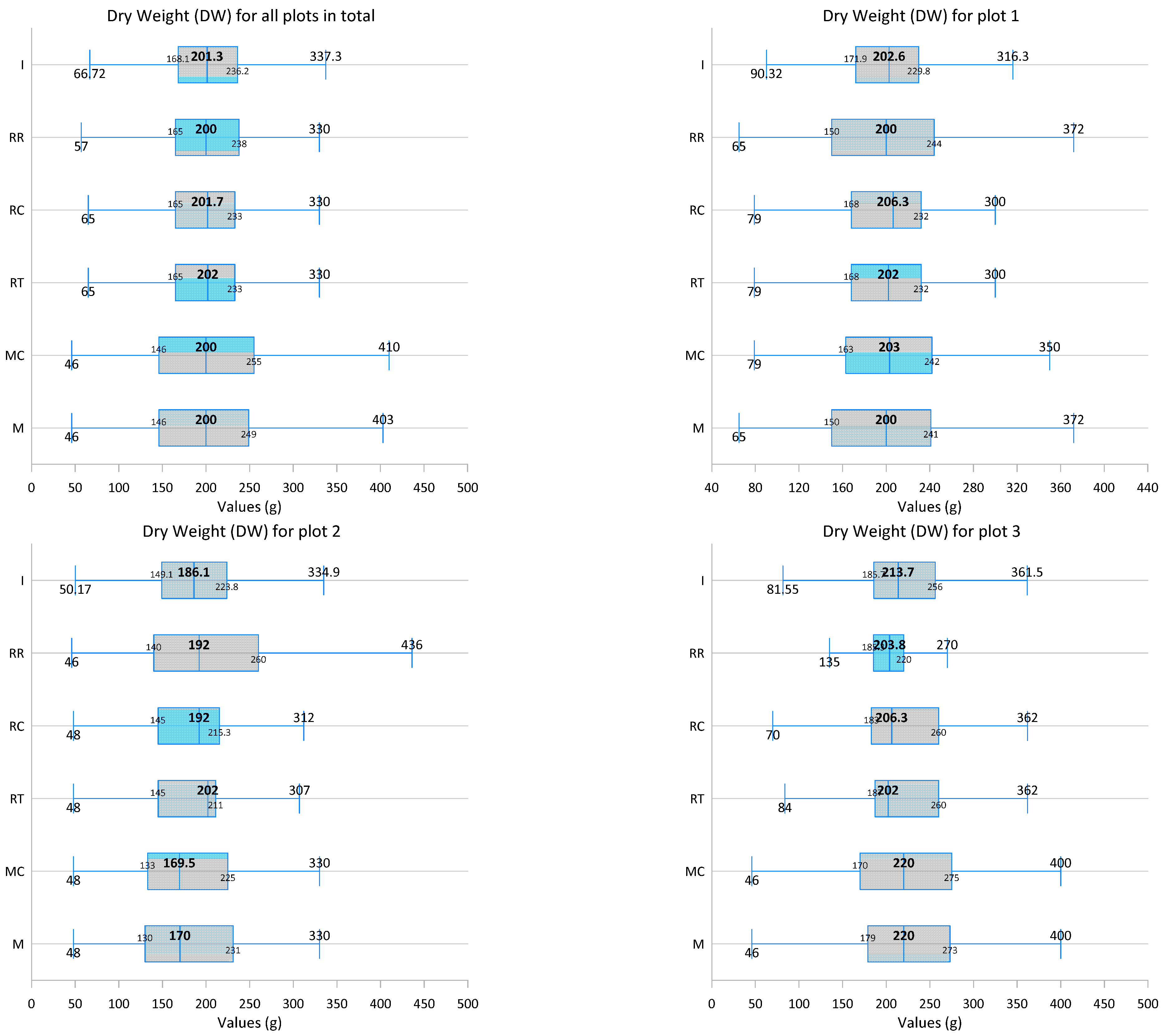
| All Plots | Plot 1 | |||||||||||
|---|---|---|---|---|---|---|---|---|---|---|---|---|
| M | MC | RT | RC | RR | I | M | MC | RT | RC | RR | I | |
| Min | 46.0 | 46.0 | 46.0 | 46.0 | 46.0 | 50.2 | 65.0 | 79.0 | 65.0 | 65.0 | 65.0 | 76.6 |
| Q1 | 146.5 | 147.0 | 165.0 | 165.0 | 165.0 | 168.1 | 150.0 | 163.3 | 168.5 | 168.5 | 150.0 | 171.9 |
| Median | 200.0 | 200.0 | 202.0 | 201.7 | 200.0 | 201.3 | 200.0 | 203.0 | 202.0 | 206.3 | 200.0 | 202.6 |
| Q3 | 249.0 | 253.5 | 233.0 | 233.0 | 238.0 | 236.2 | 240.5 | 241.8 | 231.5 | 231.5 | 243.5 | 229.7 |
| Max | 464.0 | 464.0 | 464.0 | 464.0 | 464.0 | 447.5 | 410.0 | 410.0 | 410.0 | 410.0 | 410.0 | 392.6 |
| Mean | 202.0 | 202.9 | 202.0 | 202.0 | 202.1 | 203.1 | 201.3 | 205.2 | 201.5 | 201.7 | 200.4 | 201.3 |
| IQR | 102.5 | 106.5 | 68.0 | 68.0 | 73.0 | 68.1 | 90.5 | 78.5 | 63.0 | 63.0 | 93.5 | 57.8 |
| IQR/2 | 51.3 | 53.3 | 34.0 | 34.0 | 36.5 | 34.1 | 45.3 | 39.3 | 31.5 | 31.5 | 46.8 | 28.9 |
| SD | 75.8 | 78.2 | 66.5 | 66.7 | 67.3 | 53.2 | 65.3 | 67.1 | 58.1 | 58.4 | 65.9 | 45.7 |
| CV | 37.5 | 38.5 | 32.9 | 33.0 | 33.3 | 26.2 | 32.4 | 32.7 | 28.8 | 29.0 | 32.9 | 22.7 |
| KURT | 0.4 | 0.4 | 1.5 | 1.4 | 1.3 | 0.4 | 0.7 | 0.7 | 1.6 | 1.5 | 0.3 | 0.7 |
| SKEW | 0.5 | 0.5 | 0.5 | 0.5 | 0.5 | 0.3 | 0.5 | 0.6 | 0.5 | 0.5 | 0.4 | 0.3 |
| Upper Outliers (%) | 1.4 | 1.0 | 3.3 | 3.3 | 3.3 | 1.2 | 1.7 | 3.2 | 3.3 | 3.3 | 1.3 | 1.6 |
| Lower Outliers (%) | 0.0 | 0.0 | 1.6 | 1.6 | 1.3 | 0.3 | 0.0 | 0.0 | 0.7 | 0.7 | 0.0 | 0.0 |
| For the Box | ||||||||||||
| Q2-Q1 | 53.5 | 53.0 | 37.0 | 36.7 | 35.0 | 33.2 | 50.0 | 39.8 | 33.5 | 37.8 | 50.0 | 30.7 |
| Q3-Q2 | 49.0 | 53.5 | 31.0 | 31.3 | 38.0 | 34.9 | 40.5 | 38.8 | 29.5 | 25.2 | 43.5 | 27.1 |
| For the Whiskers | ||||||||||||
| Q3+1.5*IQR | 402.8 | 413.3 | 335.0 | 335.0 | 347.5 | 338.4 | 376.3 | 359.5 | 326.0 | 326.0 | 383.8 | 316.4 |
| Q1−1.5*IQR | −7.3 | −12.8 | 63.0 | 63.0 | 55.5 | 65.9 | 14.3 | 45.5 | 74.0 | 74.0 | 9.8 | 85.2 |
| Upper Whisker | 402.8 | 413.3 | 335.0 | 335.0 | 347.5 | 338.4 | 376.3 | 359.5 | 326.0 | 326.0 | 383.8 | 316.4 |
| Lower Whisker | 46.0 | 46.0 | 63.0 | 63.0 | 55.5 | 65.9 | 65.0 | 79.0 | 74.0 | 74.0 | 65.0 | 85.2 |
| Wupper-Q3 | 153.8 | 159.8 | 102.0 | 102.0 | 109.5 | 102.2 | 135.8 | 117.8 | 94.5 | 94.5 | 140.3 | 86.7 |
| Q1-Wlower | 100.5 | 101.0 | 102.0 | 102.0 | 109.5 | 102.2 | 85.0 | 84.3 | 94.5 | 94.5 | 85.0 | 86.7 |
| Plot 2 | Plot 3 | |||||||||||
| M | MC | RT | RC | RR | I | M | MC | RT | RC | RR | I | |
| Min | 48.0 | 48.0 | 48.0 | 48.0 | 46.0 | 50.2 | 46.0 | 46.0 | 46.0 | 46.0 | 84.0 | 54.2 |
| Q1 | 131.5 | 133.0 | 145.3 | 145.3 | 140.0 | 149.1 | 177.0 | 170.5 | 187.8 | 183.0 | 185.3 | 185.6 |
| Median | 170.0 | 169.5 | 202.0 | 192.0 | 192.0 | 186.1 | 220.0 | 220.0 | 202.0 | 206.3 | 203.8 | 213.7 |
| Q3 | 228.0 | 225.0 | 210.5 | 215.3 | 259.3 | 223.8 | 271.5 | 274.0 | 259.3 | 259.3 | 220.0 | 256.0 |
| Max | 436.0 | 436.0 | 436.0 | 436.0 | 464.0 | 398.6 | 464.0 | 464.0 | 464.0 | 464.0 | 362.0 | 447.5 |
| Mean | 180.4 | 179.2 | 186.0 | 185.8 | 201.5 | 188.6 | 223.5 | 223.5 | 218.6 | 218.6 | 204.4 | 219.4 |
| IQR | 96.5 | 92.0 | 65.3 | 70.0 | 119.3 | 74.7 | 94.5 | 103.5 | 71.5 | 76.3 | 34.8 | 70.3 |
| IQR/2 | 48.3 | 46.0 | 32.6 | 35.0 | 59.6 | 37.3 | 47.3 | 51.8 | 35.8 | 38.1 | 17.4 | 35.2 |
| SD | 75.4 | 77.0 | 65.5 | 65.8 | 87.4 | 54.3 | 80.8 | 83.1 | 71.5 | 71.7 | 40.7 | 54.6 |
| CV | 41.8 | 43.0 | 35.2 | 35.4 | 43.4 | 28.8 | 36.1 | 37.2 | 32.7 | 32.8 | 19.9 | 24.9 |
| KURT | 0.5 | 0.7 | 1.4 | 1.3 | 0.2 | 0.0 | 0.4 | 0.3 | 1.3 | 1.3 | 3.5 | 0.5 |
| SKEW | 0.6 | 0.7 | 0.4 | 0.4 | 0.5 | 0.3 | 0.3 | 0.3 | 0.5 | 0.5 | 0.7 | 0.3 |
| Upper Outliers (%) | 1.8 | 2.0 | 3.3 | 2.0 | 1.3 | 0.5 | 1.7 | 1.9 | 3.3 | 3.3 | 4.7 | 1.0 |
| Lower Outliers (%) | 0.0 | 0.0 | 0.0 | 0.0 | 0.0 | 0.0 | 0.0 | 0.0 | 2.7 | 1.3 | 4.0 | 0.5 |
| For the Box | ||||||||||||
| Q2-Q1 | 38.5 | 36.5 | 56.8 | 46.8 | 52.0 | 37.0 | 43.0 | 49.5 | 14.3 | 23.3 | 18.5 | 28.0 |
| Q3-Q2 | 58.0 | 55.5 | 8.5 | 23.3 | 67.3 | 37.7 | 51.5 | 54.0 | 57.3 | 53.0 | 16.2 | 42.3 |
| For the Whiskers | ||||||||||||
| Q3+1.5*IQR | 372.8 | 363.0 | 308.4 | 320.3 | 438.1 | 335.8 | 413.3 | 429.3 | 366.5 | 373.6 | 272.1 | 361.5 |
| Q1−1.5*IQR | −13.3 | −5.0 | 47.4 | 40.2 | −38.9 | 37.1 | 35.3 | 15.3 | 80.5 | 68.6 | 133.1 | 80.1 |
| Upper Whisker | 372.8 | 363.0 | 308.4 | 320.3 | 438.1 | 335.8 | 413.3 | 429.3 | 366.5 | 373.6 | 272.1 | 361.5 |
| Lower Whisker | 48.0 | 48.0 | 48.0 | 48.0 | 46.0 | 50.2 | 46.0 | 46.0 | 80.5 | 68.6 | 133.1 | 80.1 |
| Wupper-Q3 | 144.8 | 138.0 | 97.9 | 105.0 | 178.9 | 112.0 | 141.8 | 155.3 | 107.3 | 114.4 | 52.1 | 105.5 |
| Q1-Wlower | 83.5 | 85.0 | 97.3 | 97.3 | 94.0 | 98.9 | 131.0 | 124.5 | 107.3 | 114.4 | 52.1 | 105.5 |
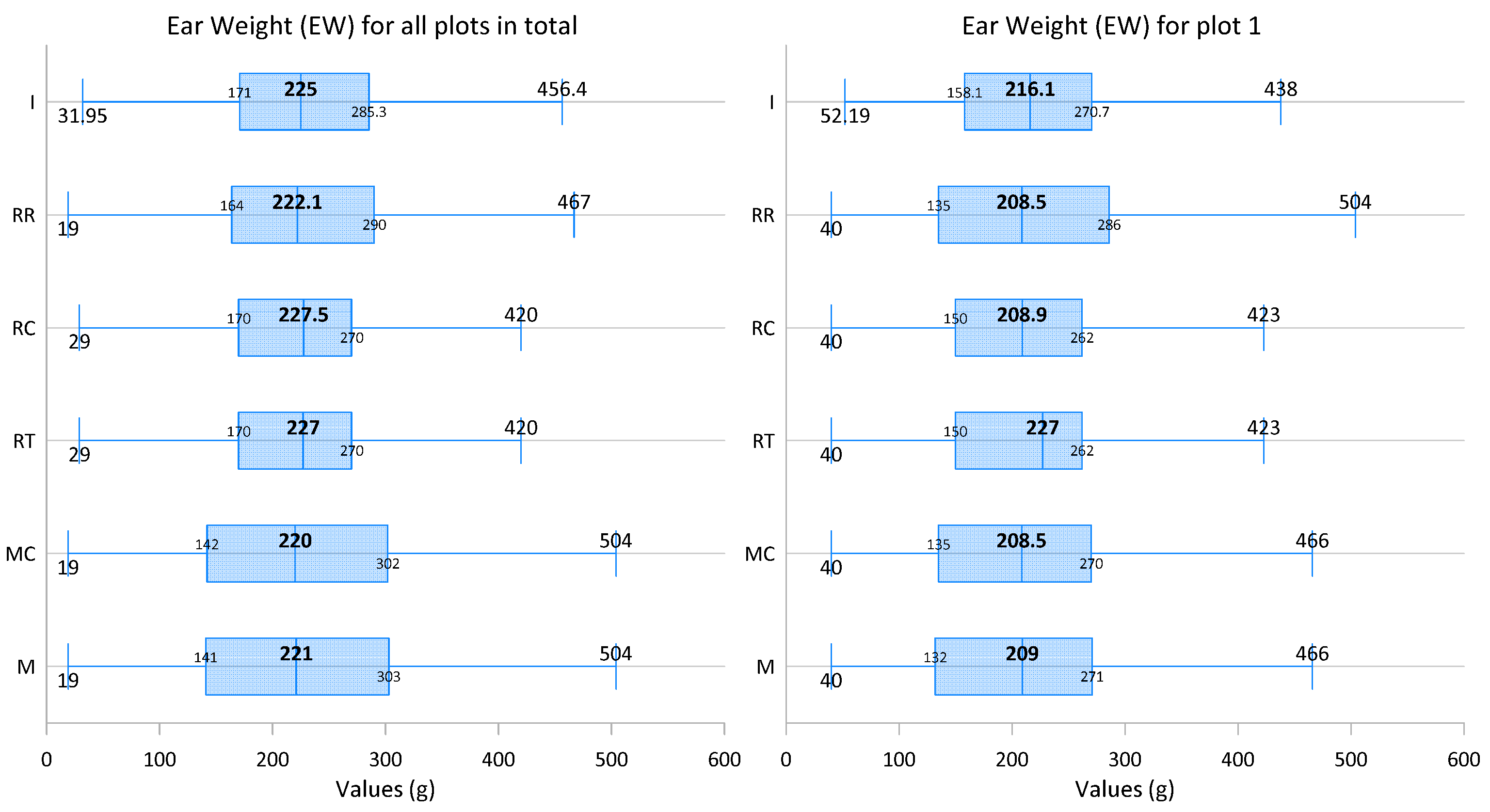
| M | MC | RT | RC | RR | I | M | MC | RT | RC | RR | I | |
|---|---|---|---|---|---|---|---|---|---|---|---|---|
| Min | 19.0 | 19.0 | 19.0 | 19.0 | 19.0 | 32.0 | 40.0 | 40.0 | 40.0 | 40.0 | 40.0 | 52.2 |
| Q1 | 141.3 | 144.0 | 170.0 | 170.0 | 164.8 | 171.0 | 133.5 | 135.3 | 150.0 | 150.0 | 135.3 | 158.1 |
| Median | 221.0 | 220.0 | 227.0 | 227.5 | 222.1 | 225.0 | 209.0 | 208.5 | 227.0 | 208.9 | 208.5 | 216.1 |
| Q3 | 302.8 | 301.5 | 270.0 | 270.0 | 290.0 | 285.2 | 270.5 | 270.0 | 261.5 | 261.5 | 285.0 | 270.6 |
| Max | 572.0 | 572.0 | 572.0 | 572.0 | 572.0 | 562.3 | 572.0 | 572.0 | 572.0 | 572.0 | 572.0 | 562.3 |
| Mean | 226.9 | 226.5 | 226.9 | 227.9 | 227.4 | 230.3 | 217.3 | 216.6 | 219.3 | 219.7 | 218.0 | 221.1 |
| IQR | 161.5 | 157.5 | 100.0 | 100.0 | 125.3 | 114.3 | 137.0 | 134.8 | 111.5 | 111.5 | 149.8 | 112.5 |
| IQR/2 | 80.8 | 78.8 | 50.0 | 50.0 | 62.6 | 57.1 | 68.5 | 67.4 | 55.8 | 55.8 | 74.9 | 56.3 |
| SD | 111.4 | 112.4 | 97.6 | 98.2 | 99.4 | 82.5 | 115.3 | 115.7 | 102.7 | 103.3 | 112.3 | 87.7 |
| CV | 49.1 | 49.6 | 43.0 | 43.1 | 43.7 | 35.8 | 53.1 | 53.4 | 46.8 | 47.0 | 51.5 | 39.7 |
| KURT | −0.4 | −0.4 | 0.4 | 0.3 | 0.2 | −0.1 | 0.1 | 0.3 | 0.8 | 0.7 | 0.0 | 0.6 |
| SKEW | 0.3 | 0.3 | 0.3 | 0.3 | 0.3 | 0.3 | 0.7 | 0.7 | 0.7 | 0.6 | 0.6 | 0.6 |
| Upper Outliers (%) | 0.3 | 0.3 | 4.0 | 4.0 | 1.6 | 0.5 | 3.4 | 3.2 | 4.0 | 4.0 | 0.7 | 2.1 |
| Lower Outliers (%) | 0.0 | 0.0 | 0.4 | 0.4 | 0.0 | 0.0 | 0.0 | 0.0 | 0.0 | 0.0 | 0.0 | 0.0 |
| For the Box | ||||||||||||
| Q2-Q1 | 79.8 | 76.0 | 57.0 | 57.5 | 57.3 | 54.0 | 75.5 | 73.3 | 77.0 | 58.9 | 73.3 | 58.0 |
| Q3-Q2 | 81.8 | 81.5 | 43.0 | 42.5 | 67.9 | 60.2 | 61.5 | 61.5 | 34.5 | 52.6 | 76.5 | 54.5 |
| For the Whiskers | ||||||||||||
| Q3+1.5*IQR | 545.0 | 537.8 | 420.0 | 420.0 | 477.9 | 456.6 | 476.0 | 472.1 | 428.8 | 428.8 | 509.6 | 439.5 |
| Q1−1.5*IQR | −101.0 | −92.3 | 20.0 | 20.0 | −23.1 | −0.4 | −72.0 | −66.9 | −17.3 | −17.3 | −89.4 | −10.7 |
| Upper Whisker | 545.0 | 537.8 | 420.0 | 420.0 | 477.9 | 456.6 | 476.0 | 472.1 | 428.8 | 428.8 | 509.6 | 439.5 |
| Lower Whisker | 19.0 | 19.0 | 20.0 | 20.0 | 19.0 | 32.0 | 40.0 | 40.0 | 40.0 | 40.0 | 40.0 | 52.2 |
| Wupper-Q3 | 242.3 | 236.3 | 150.0 | 150.0 | 187.9 | 171.4 | 205.5 | 202.1 | 167.3 | 167.3 | 224.6 | 168.8 |
| Q1-Wlower | 122.3 | 125.0 | 150.0 | 150.0 | 145.8 | 139.0 | 93.5 | 95.3 | 110.0 | 110.0 | 95.3 | 105.9 |
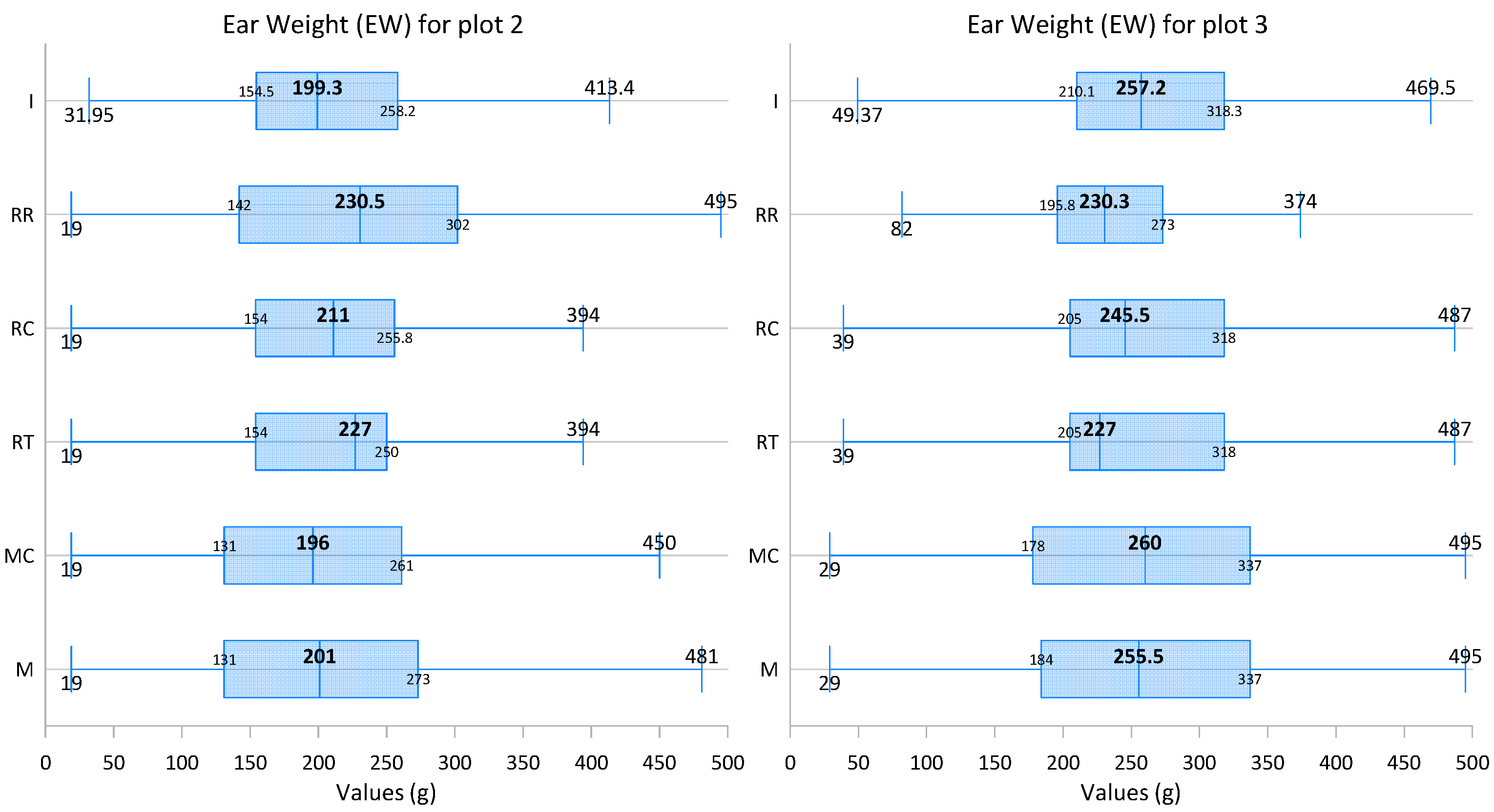
| Plot 2 | Plot 3 | |||||||||||
| M | MC | RT | RC | RR | I | M | MC | RT | RC | RR | I | |
| Min | 19.0 | 19.0 | 19.0 | 19.0 | 19.0 | 32.0 | 29.0 | 29.0 | 29.0 | 29.0 | 82.0 | 43.2 |
| Q1 | 131.5 | 131.3 | 154.3 | 154.3 | 144.0 | 154.5 | 183.5 | 181.0 | 205.5 | 205.1 | 195.8 | 210.0 |
| Median | 201.0 | 196.0 | 227.0 | 211.0 | 230.5 | 199.3 | 255.5 | 260.0 | 227.0 | 245.5 | 230.3 | 257.2 |
| Q3 | 270.5 | 260.8 | 249.8 | 255.8 | 301.8 | 258.0 | 336.3 | 336.5 | 316.8 | 316.8 | 270.8 | 318.2 |
| Max | 481.0 | 481.0 | 481.0 | 481.0 | 495.0 | 464.7 | 495.0 | 495.0 | 495.0 | 495.0 | 439.0 | 469.5 |
| Mean | 207.1 | 205.3 | 212.3 | 213.0 | 227.7 | 209.5 | 255.7 | 255.8 | 249.2 | 251.0 | 236.5 | 260.3 |
| IQR | 139.0 | 129.5 | 95.5 | 101.5 | 157.8 | 103.5 | 152.8 | 155.5 | 111.3 | 111.7 | 75.0 | 108.2 |
| IQR/2 | 69.5 | 64.8 | 47.8 | 50.8 | 78.9 | 51.8 | 76.4 | 77.8 | 55.6 | 55.8 | 37.5 | 54.1 |
| SD | 103.7 | 103.9 | 89.5 | 90.4 | 112.3 | 75.9 | 109.5 | 112.0 | 97.0 | 97.1 | 65.9 | 74.5 |
| CV | 50.1 | 50.6 | 42.2 | 42.4 | 49.3 | 36.2 | 42.8 | 43.8 | 38.9 | 38.7 | 27.9 | 28.6 |
| KURT | −0.1 | 0.1 | 0.8 | 0.6 | −0.5 | 0.1 | −0.6 | −0.6 | 0.0 | 0.0 | 1.1 | −0.4 |
| SKEW | 0.4 | 0.5 | 0.3 | 0.2 | 0.1 | 0.5 | −0.2 | −0.2 | 0.0 | 0.0 | 0.7 | −0.2 |
| Upper Outliers (%) | 0.9 | 3.1 | 4.0 | 3.3 | 0.0 | 0.9 | 0.0 | 0.0 | 1.3 | 1.3 | 4.0 | 0.0 |
| Lower Outliers (%) | 0.0 | 0.0 | 0.0 | 0.0 | 0.0 | 0.0 | 0.0 | 0.0 | 2.7 | 2.7 | 0.7 | 0.1 |
| For the Box | ||||||||||||
| Q2-Q1 | 69.5 | 64.8 | 72.8 | 56.8 | 86.5 | 44.8 | 72.0 | 79.0 | 21.5 | 40.4 | 34.5 | 47.2 |
| Q3-Q2 | 69.5 | 64.8 | 22.8 | 44.8 | 71.3 | 58.7 | 80.8 | 76.5 | 89.8 | 71.3 | 40.4 | 61.0 |
| For the Whiskers | ||||||||||||
| Q3+1.5*IQR | 479.0 | 455.0 | 393.0 | 408.0 | 538.4 | 413.3 | 565.4 | 569.8 | 483.6 | 484.2 | 383.2 | 480.5 |
| Q1−1.5*IQR | −77.0 | −63.0 | 11.0 | 2.0 | −92.6 | −0.8 | −45.6 | −52.3 | 38.6 | 37.6 | 83.3 | 47.8 |
| Upper Whisker | 479.0 | 455.0 | 393.0 | 408.0 | 495.0 | 413.3 | 495.0 | 495.0 | 483.6 | 484.2 | 383.2 | 469.5 |
| Lower Whisker | 19.0 | 19.0 | 19.0 | 19.0 | 19.0 | 32.0 | 29.0 | 29.0 | 38.6 | 37.6 | 83.3 | 47.8 |
| Wupper-Q3 | 208.5 | 194.3 | 143.3 | 152.3 | 193.3 | 155.3 | 158.8 | 158.5 | 166.9 | 167.5 | 112.4 | 151.3 |
| Q1-Wlower | 112.5 | 112.3 | 135.3 | 135.3 | 125.0 | 122.5 | 154.5 | 152.0 | 166.9 | 167.5 | 112.4 | 162.3 |
| All Plots | M | MC | MC+ Diff% from M | RT | RT Diff% from M | RC | RC Diff% from M | RR | RR Diff% from M | I | I Diff% from M |
|---|---|---|---|---|---|---|---|---|---|---|---|
| FW | 38.6 | 39.3 | 1.9 | 34.1 | 11.7 | 34.1 | 11.5 | 34.4 | 10.8 | 27.5 | 28.9 |
| DW | 37.5 | 38.5 | 2.6 | 32.9 | 12.3 | 33.0 | 12.0 | 33.3 | 11.3 | 26.2 | 30.2 |
| EW | 49.1 | 49.6 | 1.1 | 43.0 | 12.4 | 43.1 | 12.2 | 43.7 | 11.0 | 35.8 | 27.0 |
| Plot 1 | M | MC | MC Diff% from M | RT | RT Diff% from M | RC | RC Diff% from M | RR | RR Diff% from M | I | I Diff% from M |
| FW | 36.9 | 37.3 | 1.0 | 32.8 | 11.3 | 32.8 | 11.0 | 36.8 | 0.5 | 27.2 | 26.3 |
| DW | 32.4 | 32.7 | 0.8 | 28.8 | 11.1 | 29.0 | 10.7 | 32.9 | 1.4 | 22.7 | 30.0 |
| EW | 53.1 | 53.4 | 0.7 | 46.8 | 11.8 | 47.0 | 11.4 | 51.5 | 2.9 | 39.7 | 25.2 |
| Plot 2 | M | MC | MC Diff% from M | RT | RT Diff% from M | RC | RC Diff% from M | RR | RR Diff% from M | I | I Diff% from M |
| FW | 41.6 | 42.5 | 2.0 | 35.1 | 15.6 | 35.3 | 15.2 | 42.0 | 0.8 | 29.2 | 29.8 |
| DW | 41.8 | 43.0 | 2.7 | 35.2 | 15.8 | 35.4 | 15.3 | 43.4 | 3.7 | 28.8 | 31.1 |
| EW | 50.1 | 50.6 | 1.1 | 42.2 | 15.8 | 42.4 | 15.3 | 49.3 | 1.4 | 36.2 | 27.6 |
| Plot 3 | M | MC | MC Diff% from M | RT | RT Diff% from M | RC | RC Diff% from M | RR | RR Diff% from M | I | I Diff% from M |
| FW | 35.6 | 36.4 | 2.3 | 32.8 | 7.9 | 32.8 | 7.8 | 21.5 | 39.6 | 23.6 | 33.7 |
| DW | 36.1 | 37.2 | 2.9 | 32.7 | 9.5 | 32.8 | 9.2 | 19.9 | 44.9 | 24.9 | 31.1 |
| EW | 42.8 | 43.8 | 2.2 | 38.9 | 9.2 | 38.7 | 9.7 | 27.9 | 34.9 | 28.6 | 33.2 |
| All Plots | M | MC | Diff% | RT | Diff% | RC | Diff% | RR | Diff% | I | Diff% |
|---|---|---|---|---|---|---|---|---|---|---|---|
| FW | 659.5 | 661.9 | 0.4 | 659.4 | 0.0 | 660.4 | 0.1 | 660.0 | 0.1 | 665.5 | 0.9 |
| DW | 202.0 | 202.9 | 0.4 | 202.0 | 0.0 | 202.0 | 0.0 | 202.1 | 0.0 | 203.1 | 0.5 |
| EW | 226.9 | 226.5 | −0.2 | 226.9 | 0.0 | 227.9 | 0.5 | 227.4 | 0.2 | 230.3 | 1.5 |
| Plot 1 | M | MC | Diff% | RT | Diff% | RC | Diff% | RR | Diff% | I | Diff% |
| FW | 648.6 | 657.5 | 1.4 | 650.7 | 0.3 | 652.2 | 0.6 | 646.2 | −0.4 | 654.7 | 0.9 |
| DW | 201.3 | 205.2 | 1.9 | 201.5 | 0.1 | 201.7 | 0.2 | 200.4 | −0.4 | 201.3 | 0.0 |
| EW | 217.3 | 216.6 | −0.3 | 219.3 | 0.9 | 219.7 | 1.1 | 218.0 | 0.4 | 221.1 | 1.8 |
| Plot 2 | M | MC | Diff% | RT | Diff% | RC | Diff% | RR | Diff% | I | Diff% |
| FW | 597.6 | 593.3 | −0.7 | 613.5 | 2.7 | 614.6 | 2.9 | 659.3 | 10.3 | 613.6 | 2.7 |
| DW | 180.4 | 179.2 | −0.7 | 186.0 | 3.1 | 185.8 | 3.0 | 201.5 | 11.7 | 188.6 | 4.5 |
| EW | 207.1 | 205.3 | −0.9 | 212.3 | 2.5 | 213.0 | 2.9 | 227.7 | 9.9 | 209.5 | 1.1 |
| Plot 3 | M | MC | Diff% | RT | Diff% | RC | Diff% | RR | Diff% | I | Diff% |
| FW | 729.9 | 731.1 | 0.2 | 716.1 | −1.9 | 716.6 | −1.8 | 675.2 | −7.5 | 728.1 | −0.2 |
| DW | 223.5 | 223.5 | 0.0 | 218.6 | −2.2 | 218.6 | −2.2 | 204.4 | −8.5 | 219.4 | −1.8 |
| EW | 255.7 | 255.8 | 0.1 | 249.2 | −2.5 | 251.0 | −1.8 | 236.5 | −7.5 | 260.3 | 1.8 |
Publisher’s Note: MDPI stays neutral with regard to jurisdictional claims in published maps and institutional affiliations. |
© 2022 by the authors. Licensee MDPI, Basel, Switzerland. This article is an open access article distributed under the terms and conditions of the Creative Commons Attribution (CC BY) license (https://creativecommons.org/licenses/by/4.0/).
Share and Cite
Koutsos, T.M.; Menexes, G.C.; Eleftherohorinos, I.G. The Use of Spatial Interpolation to Improve the Quality of Corn Silage Data in Case of Presence of Extreme or Missing Values. ISPRS Int. J. Geo-Inf. 2022, 11, 153. https://doi.org/10.3390/ijgi11030153
Koutsos TM, Menexes GC, Eleftherohorinos IG. The Use of Spatial Interpolation to Improve the Quality of Corn Silage Data in Case of Presence of Extreme or Missing Values. ISPRS International Journal of Geo-Information. 2022; 11(3):153. https://doi.org/10.3390/ijgi11030153
Chicago/Turabian StyleKoutsos, Thomas M., Georgios C. Menexes, and Ilias G. Eleftherohorinos. 2022. "The Use of Spatial Interpolation to Improve the Quality of Corn Silage Data in Case of Presence of Extreme or Missing Values" ISPRS International Journal of Geo-Information 11, no. 3: 153. https://doi.org/10.3390/ijgi11030153
APA StyleKoutsos, T. M., Menexes, G. C., & Eleftherohorinos, I. G. (2022). The Use of Spatial Interpolation to Improve the Quality of Corn Silage Data in Case of Presence of Extreme or Missing Values. ISPRS International Journal of Geo-Information, 11(3), 153. https://doi.org/10.3390/ijgi11030153