Crowd Anomaly Detection via Spatial Constraints and Meaningful Perturbation

Abstract

Crowd anomaly detection is a practical and challenging problem to computer vision and VideoGIS due to abnormal events’ rare and diverse nature. Consequently, traditional methods rely on low-level reconstruction in a single image space, easily affected by unimportant pixels or sudden variations. In addition, real-time detection for crowd anomaly detection is challenging, and localization of anomalies requires other supervision. We present a new detection approach to learn spatiotemporal features with the spatial constraints of a still dynamic image. First, a lightweight spatiotemporal autoencoder has been proposed, capable of real-time image reconstruction. Second, we offer a dynamic network to obtain a compact representation of video frames in motion, reducing false-positive anomaly alerts by spatial constraints. In addition, we adopt the perturbation visual interpretation method for anomaly visualization and localization to improve the credibility of the results. In experiments, our results provide competitive performance across various scenarios. Besides, our approach can process 52.9–63.4 fps in anomaly detection, making it practical for crowd anomaly detection in video surveillance.

1. Introduction

Video data have become indispensable in the monitoring of public safety. It also provides unprecedented opportunities for GIS to investigate the processes that govern the dynamics of collective social phenomena [1]. A significant focus is crowd anomaly detection. For example, video surveillance should detect violent conflict or traffic accidents quickly and accurately. Traditional approaches are severely limited by the amount of human effort required to manually perform decision making. However, as tasks become more complex and the number of options to reason about becomes more remarkable, there is an increasing need to specify the desired abnormalities in an automated and interpretable fashion.

Since abnormal event footage in video sequences is infrequent, detection has often been performed with one-class classifiers [2]. Recently, reconstruction-based models [3,4,5,6] have become the most promising solution. These studies send regular frames or spatiotemporal features to the framework and reconstruct them with minor errors. Therefore, anomalies usually exhibit more significant reconstruction errors due to deviations from standard visual patterns. However, abnormal events can also be reconstructed because of deep neural networks’ large capacity and generalization. In addition, it is not feasible to collect all possible regular scenarios for training; the normal class may also be different from the learned representations and may be detected as anomalous. The second category is prediction-based methods. They predict future frames [7,8,9] with a variational autoencoder (VAE). Therefore, the predicted frames achieved greater feasible possibilities and promoted video detection performance based on the generative adversarial network (GAN) [10].

Although the above methods allow us to automatically conduct anomaly detection tasks with video surveillance, the detection performance of current approaches remains restricted. First, most techniques learn regular patterns and detect anomalies within a single, appearance-based image space. They usually compare the raw video frames with the reconstructed frames pixel-by-pixel, which is susceptible to unimportant pixels or sudden variations. Second, their computational cost in processing high-dimensional video frames is high and not applicable to real-time applications. In addition, these approaches always left how classification interacts with scene semantics unclear; there is a need to develop methods that provide predictive guarantees to make the models trustworthy for surveillance. Therefore, a significant effort in exploring the practical approach of crowd anomaly detection is required to fill the research gap between computational complexity and detection effectiveness.

Here, we tackle the above questions and narrow the gap with a new lightweight framework for crowd anomaly detection and localization. First, we proposed a lightweight framework containing a low-dimensional autoencoder and a dynamic map approximator, and multiple aggregating objectives that exploit motion, appearance, perturbation, and dynamic features. Second, we defined the regularity score with spatial constraints using the dynamic map, reducing false-positive alerts due to motion blur, sudden variations, etc. Additionally, we present a perturbed visual interpretation method for the visualization and localization of anomalies. It does not require other supervision and is easy to embed in existing networks.

The main novelties in our work are highlighted as follows: (1) It formulates a lightweight structure with multiple objectives, which can narrow down the comparison space and filter unimportant pixels or sudden variations. (2) It designs an algorithm’s interpretation using meaningful perturbation, making visual features have clear semantic connotations and enabling the localization of anomaly detection. (3) It refined effective detection to a feasible pattern with low computational costs scales to meet real-time crowd surveillance. That is to say, our approach is the aggregation of multiple objectives that exploits motion, appearance, perturbation, and dynamic features to narrow the gap between computational complexity and detection effectiveness. From a practical perspective, the application of our approach could improve ongoing video surveillance for crowd anomaly detection.

2. Literature Review

The proposed method deals with a challenging detection task: specifying the desired abnormalities as automated and interpretable, narrowing the gap between computational complexity and detection effectiveness. From a practical aspect, the extension includes two significant elements.

2.1. Crowd Anomaly Detection

Crowd anomaly detection is a primary task in public safety. It is a complex task as the anomalies are not known beforehand. Recent studies mainly focus on hand-crafted video features [11,12] and deep learning [13]. Since abnormal event footage in video sequences is rare, weak-supervised anomy detection methods are widely used. For example, interaction energy [14,15], spatiotemporal features [16,17], dictionary learning [18], and sparse representation [19,20] only analyze the distribution of regular data and signify the anomaly score while testing. Most of the weakly supervised models in anomaly detection suggested that the model can be trained from reconstruction works [21,22,23]. For example, Xu et al. [24] proposed a method to learn specific descriptors of the scene of interest. Luo et al. [25] established an LSTM-based detection framework, reconstructing the previous video frame and predicting the subsequent video frame through hidden vectors. On this basis, Wang et al. [26] proposed an optimized forecasting method to distinguish between normal and abnormal events significantly. Zhou et al. [27] obtained effective motion blocks by segmenting the motion area and the algorithm used the per-class classifier to model each sample. Li et al. [28] proposed a framework quantifying and detecting collective motion in crowd scenes. Thus, they achieve abnormal event detection in the crowd while simultaneously considering the appearance and motion patterns. Some effort has been taken to detect each input object’s elements [29,30], improving the fully convolutional neural network and generating adversarial networks. These architectures can show abnormal areas but fail to express the temporal correlation between video frames. Thus, several authors have recently presented a two-stream convolutional network for abnormal detection, including the composition of an appearance stream and action stream [31], which improved details in the output frames [32]. Since most previous methods concentrate on modeling motion patterns [33], one universal limitation is that labeled data are needed to train the normal or abnormal pattern and limit the applicability of these methods in practical applications. The challenge, therefore, in practical applications is in online detection. These ideas have motivated the incremental spatiotemporal learner [34] and particle-filtering-based anomaly detection algorithm [35]; however, they depend on human feedback, not an end-to-end approach.

These studies mainly focused on high-dimensional, single image spaces, and the preservation of all detailed information. In contrast, we learn spatiotemporal features and dynamic images from different perspectives. We present a low-dimensional autoencoder to reduce computational complexity and a dynamic pattern to narrow down the comparison space and reduce the gap between complexity and efficiency.

2.2. Crowd Anomaly Localization

Identifying anomaly locations will be essential to better the system’s visibility and status. Advances in deep CNNs have verified the effectiveness of this task. For instance, Zhu et al. [36] introduced a motion augmented network for better localizing anomalies. Considering the competitive cascade of DNNs, Sabokrou et al. [37] describe a cubic-patch-based method. They divide the framework into two sub-stages and operate as cascaded classifiers. Furthermore, Lv. et al. [38] proposed a weakly supervised method to detect anomaly locations using video-level labels. Thus, the extracted semantics can directly cue to infer anomalies. In addition, Ahmed et al. [39] proposed a data-driven approach to enable anomaly detection and localization. The localization task is performed using the anomaly score. Based on the generation method, Aramith. et al. [40] proposed edge wrapping to reduce the noise and suppress nonrelated edges of anomaly objects. Muhammad et al. [41] used SqueezeNet with smaller convolutional kernels without dense fire localization in surveillance video. Anomaly localization can also be categorized into an interpretation task. Modeling visualization and explanation have experienced tremendous advances in computer vision [42,43]. Policymakers need to decide among many possible meanings of interpretability. These range from visualization [44,45,46] and post hoc interpretations of decisions [47] to assure that the results are reliable in terms of the specified objectives [48]. However, methods that produce intuitive visualization are primarily heuristic, opaque, nonintuitive, and difficult for analysts to understand the inner decision reason [49,50].

In summary, the current literature for localization of anomaly detection is mainly limited to other forms of supervision. In contrast, we propose a pixel-level interpretation map by adding perturbation items to the input image. Moreover, we obtain a fine-grained approximate solution to the “black-box” issue and localize anomaly regions.

3. Materials and Methods

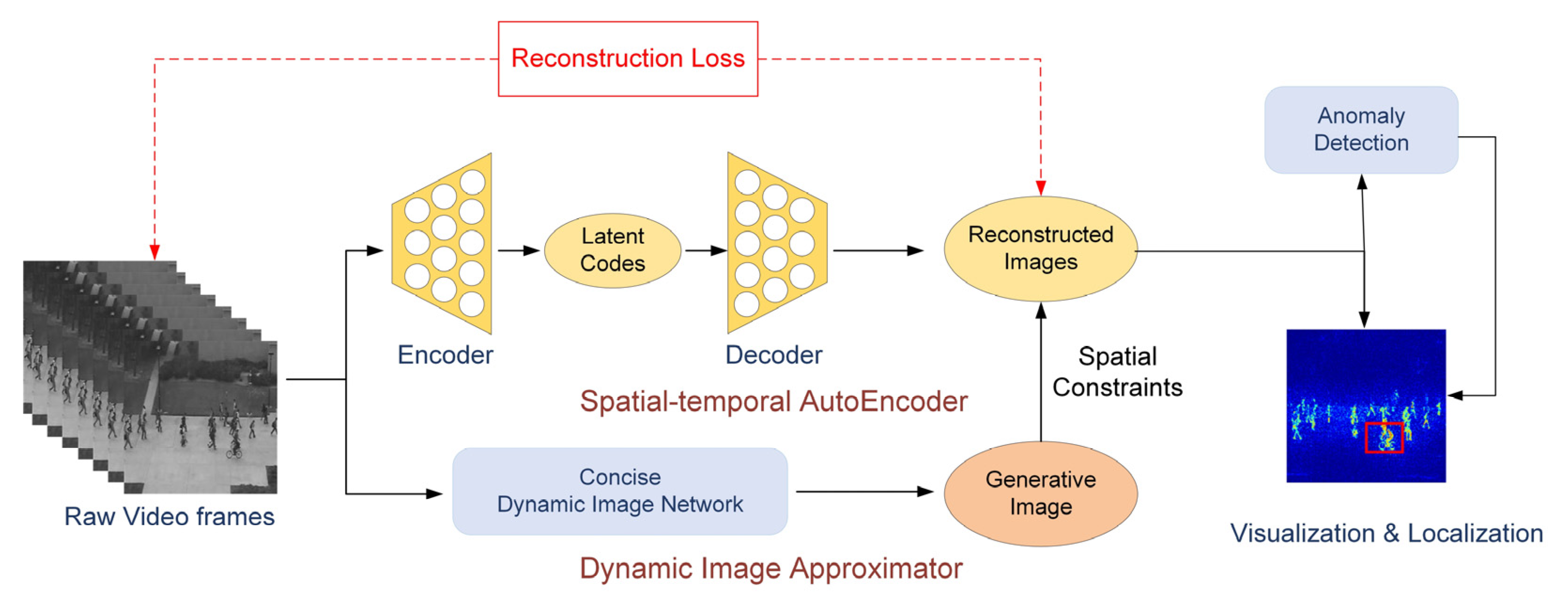
3.1. Overview

Intuitively, only a few actions can cause anomalies for a particular crowd scenario, and the appearance and motion of visual objects are critical to anomaly detection. To this end, the proposed approach applies to real-time anomaly detection and localization over video surveillance. Figure 1 presents the overview of our method. It is composed of an autoencoder and a generator. More specifically, the autoencoder is modified to two-dimensional space, the shortcut of which can contribute to both accuracy and efficiency. Besides, we utilize dynamic images to represent the reconstructed frame’s spatial constraints and expect visualization and localization for anomalies using meaningful perturbation.

The main differences between our approach and former methods include two main components. First, our approach narrows down the comparison space by distilling the dynamic area and filtering unimportant pixels or sudden variations. (The dynamic image approach is usually used to compact video representation). Second, we use the perturbation method to explain the decision process and its corresponding localization to guide object-level anomaly detection.

3.2. Problem Statements

A key driver for the advancement of deep learning for crowd anomaly research will be to narrow the gap between computational complexity and detection effectiveness and satisfy the demand for explainability.

Here, we assume that only a limited dynamic area can cause anomalies for a particular surveillance scenario in this work. Therefore, resenting the anomaly detection with spatial constraints might narrow the gap between computational complexity and detection effectiveness. This is reasonable because the structure of anomaly detection can incorporate powerful deep learning capabilities and high-level dependencies from geospatial data. First, keeping the low-dimensional encoder and decoder can notably reduce computation complexity during spatiotemporal features detection. Second, the dynamic image approximator could narrow the pixel-by-pixel comparison area onto a specific image space, filtering unimportant pixels or sudden variations.

In addition to ensuring complexity and effectiveness, there is a growing demand to explain the systems’ decisions. Anomaly detection learns the relationships between data inputs and decision outputs from a practical perspective. Thus, explainability can enable model trustworthiness and visualization. A fundamental element of the demand for explainability is to assure that outcomes are fair for the specified individuals for the decision.

3.3. Spatiotemporal Autoencoder with Dynamic Map Approximation

3.3.1. Basic Concepts

The proposed module consists of the spatiotemporal autoencoder and dynamic image approximator that jointly investigate the representative and image dynamics, as illustrated in Figure 2. Let $I\left(\mathrm{x},\mathrm{t}\right)$ be a video frame on spatial domain D and temporal domain T, where $\mathrm{x}\in \mathrm{D}$ indicates the pixel coordinates, and $\mathrm{t}\in \mathrm{T}$ indicates the frames in the video sequence. Thus, $I\left(\mathrm{x},\mathrm{t}\right)$ can be a three-dimensional function on D × T.

3.3.2. Spatiotemporal Autoencoder

The autoencoder is designed to exploit spatiotemporal features effectively. Its main components are described below:

Inputs: The raw video frames are preprocessed, converted into grayscale, and resized to 224 × 224 pixels to enhance the model’s capacity. The video frames are extracted as consecutive frames—eight frames per batch.

Spatial Encoder and Decoder: It consists of two convolution layers and two de-convolution layers, whose filters and kernel sizes are specified in Figure 2.

Temporal Encoder: It consists of three convLSTM layers, capturing the spatiotemporal features from the input frame sequences, whose filters and kernel sizes are specified in Figure 2.

Unlike the cubic structure, the temporal encoder generates the hidden representation of appearance features, viewed as latent representation. Given the training data x, the encoder and decoder models are parameterized by two sub-networks, $p_{\theta }(x|z)$ and $q_{\mathsf{\Phi }}\left(z|x\right)$ where $\theta$ and $\mathsf{\Phi }$ are parameters of the network and $z$ denotes a collective latent variable. Thus, the hidden representation can be obtained by:

$$q(z^a)={\displaystyle {\int }_{x^a}q(z^a|x^a)}p(x^a)d{x}^a$$

(1)

From the view of the encoder-decoder structure, we assume that the autoencoders generate the hidden representations:

$$h_i^a=g(W_{}^a{x}_i^a+b_{}^a)$$

(2)

$$h_i^m=g(W_{}^m{x}_i^m+b_{}^m)$$

(3)

where $h_i^a$ and $h_i^m$ are hidden representations for appearance and motion, respectively. The parameters $\left(W^a,W^m,b^a,b^m\right)$ are learned for a given training dataset. After that, the model realizes mappings from the spatial/temporal intrinsic representation to the spatiotemporal autoencoder. The weight matrix and bias terms of mapping are parameterized by $W^N$ and $b^N$, the mapping function is:

$$h_i^m=g(W^N{h}_i^a+b^N)$$

(4)

Based on the obtained $h_i^a$ and $h_i^m$, the optimization of the neural network in the spatiotemporal autoencoder is to learn the mapping function by minimizing:

$${\displaystyle \sum _i^n{\Vert g(W^N{h}_i^a+b^N)-h_i^m\Vert }^2}$$

(5)

To minimize the average squared error in Equation (5), we use backpropagation (BP) to adjust the parameters. We also use the spatiotemporal autoencoder to extract the regular patterns in the training procedure and control the network scale while fusing the timing information with motion. Unlike sparse reconstruction, we capture the internal relationships between video frames. The spatiotemporal filters are expected to capture the spatiotemporal patterns at multiple scales.

The lightweight structure of the spatiotemporal autoencoder indicates that the model is flexible and straightforward. It ensures that the internal representation describes spatial and temporal data well, and the neural network can learn complex relationships between the spatiotemporal terms. Moreover, the mapping function and the interior illustrations are jointly optimized and thus correlated.

3.3.3. Dynamic Image Approximator

Motion information is essential to better performance in designing a deep neural network for anomaly detection [36]. However, representing long-term dynamics is often difficult. To this end, one core task is to capture the active pattern of abnormal behavior to reveal the dynamic visual patterns of long-term appearance and motion. The dynamic map approximator compresses the video clips into a single still image while maintaining rich appearance and motion information.

Motivated by [20,51], we propose an efficient approach in which a single image summarizes the video frames. The difference is we only use the dynamic map as a mask or spatial constraints to the reconstructed frames. Let $\psi \left(I_t\right)\in {ℝ}^d$ be a vector extracted from an individual video frame $I_t$; we employ the dynamic image by compressing the video sequence into a vector of parameters d^*:

$${\mathrm{d}}^{*}=\rho (I_1,\dots ,I_T)$$

(6)

where $\rho \left(·\right)$ is the map function that maps a video sequence to a single vector, and d* can also be treated as an image. Differently, we dropped the term $\psi$ as the input to the approximator is already in the feature maps. We can also treat d* as:

$${\mathrm{d}}^{*}=\underset{\mathrm{d}}{\mathrm{argmin}}\left\{\frac{\lambda }{2}{\Vert \mathrm{d}\Vert }^2+\frac{2}{T(T-1)}\times {\displaystyle \sum _{q>t}^{}\max \{0,1-S(q|\mathrm{d})+S(t|\mathrm{d})\}}\right\}$$

(7)

where $S\left(q|\mathrm{d}\right)=\langle \mathrm{d},V_t\rangle$ is the ranking score associated with each time t and $V_t=\frac{1}{t}{\displaystyle \sum }_{r=1}^t\psi \left(I_r\right)$ is the time average of these video frames up to time t. The features reflect the order of frames in appearance, the dynamic evolution in spatial and temporal domains could be captured.

To build a spatial boundary, computing dynamic images to a high degree of accuracy may not be necessary. Thus, we use an approximation to rank pooling like [51] to optimize Equation (7), which is faster and works well in practice:

$$\mathrm{d}\propto {\displaystyle \sum _{q>t}^{}{V}_q-V_t={\displaystyle \sum _{t=1}^T{\alpha }_t{V}_t}}$$

(8)

where ${\alpha }_t$ denotes the coefficient given by ${\alpha }_t=2\left(T-t+1\right)-\left(\mathrm{T}+1\right)\left(H_T-H_{t-1}\right)$. In other words, we could recast the dynamic map approximator as a layer to fuse the appearance and motion of objects.

We devised an identity matrix $IM$ to define spatial boundaries for anomaly detection (See Figure 3). The matrix aims to identify which regions of an image are used to produce the reconstruction loss. Formally, let $I$ associate to each pixel $u$ in the dynamic image $d$ with a scalar value $m\left(u\right)$. Therefore, $IM$ is an m × n matrix similar to the dynamic image $d$. It can be computed by:

$$m(u)=\{\begin{array}{cc}1,& \mathrm{if} u \mathrm{is} \mathrm{motion} \mathrm{or} \mathrm{blur} \mathrm{in} \mathrm{image} \mathrm{space};\\ 0,& \mathrm{otherwise}.\end{array}$$

(9)

3.4. Anomaly Detection

The reconstruction error $E$ represents the difference between the raw frames and the reconstructed frames. Besides, we use spatial constraints of the dynamic map approximator to model the probability distribution of standard data. To qualitatively analyze our model, we used the regularity score to indicate our model’s ability to detect abnormalities corresponding to the normality of each frame in the video.

Using linear sampling in a video sequence reduces computation compared with a non-sampling scheme. Once trained, the reconstruction error is calculated according to the difference between the input frame and the reconstructed frame with spatial constraints. We defined the regularity score as follows:

$$\phi (k,i,j)=\{\begin{array}{cc}{\left|X_{(k,i,j)}-{\overline{X}}_{(k,i,j)}\right|}^2& I{M}_{i,j}\ge 0\\ 0& I{M}_{i,j}=0\end{array}$$

(10)

$$E(t)={\left({\displaystyle \sum _{k=0}^{N-1}{\displaystyle \sum _{i=0}^{w-1}{\displaystyle \sum _{j=0}^{h-1}\phi (k,i,j)}}}\right)}^{\frac{1}{2}}$$

(11)

where $\overline{X}$ is the reconstructed frame from $X$, $\phi \left(·\right)$ is the pixel error function, $N$ is the total frame numbers, $w$ is the width, $h$ is the height of the video frame, and $IX$ is the related identity matrix. Note that 16 frames are related to an identity matrix in our work.

By inspecting the data of where the model tended to make errors, we compute the anomaly scores $S_a\left(t\right)$, regularity scores $S_r\left(t\right)$, and then normalize the reconstruction error to [0, 1]. The calculation method of the regularity score is as follows:

$$S_a(t)=\frac{E(t)-\underset{t}{\min E}(t)}{\underset{t}{\max }E(t)-\underset{t}{\min }E(t)}$$

(12)

$$S_r\left(t\right)=1-S_a\left(t\right)$$

(13)

Suppose there is no abnormal event in a video sequence. In that case, the corresponding reconstruction error score is higher than that of the abnormal video sequence due to the absence of irregular patterns during training. Thus, setting a threshold for the regularity score can assess whether an anomalous event has occurred in a video frame. In this work, we treat the threshold as adaptive variation, calculated as follows:

$$T=a\frac{1}{N}{\displaystyle \sum }_t{S}_r\left(t\right)$$

(14)

where $S_r\left(t\right)$ denotes the regularity score, and the adjustment parameter $a$ is obtained through training.

The mentioned models also require algorithmic representations of crowd anomaly detection. The assumptions used to select these basic blocks were that only a limited dynamic area could cause anomalies for a particular surveillance scenario developed in this paper. The anomaly detection procedure is explained in Algorithm 1.

Algorithm 1. Crowd Anomaly Detection Algorithm

$\mathrm{Input}: \left\{I_t\right\}$ is a batch of raw video frames in time t Output: Anomaly video frames 1: Resize  $\left\{I_t\right\}$ to 224 × 224 pixels in Input block 2:  for each video frame  $I_i$ in $\left\{I_t\right\}$ do 3:    Forward propagate video frame  $I_i$ through Spatial Encoder block 4:    Select the feature maps SF from layer C2 of Spatial Encoder block 5:    Forward propagate SF through Temporal Encoder block 6:      if generated SFs = 16   Generate Dynamic image through Approximator block   Compute identity matrix  $I{M}_t$ from Dynamic image (Equation (9))        Initialize Dynamic image       end if 7:    Forward propagate SF through Temporal Encoder block 8:    Select the feature maps TF from layer CL3 of the Temporal Encoder block 9:    Forward propagate TF through Decoder block 10:    Select the reconstructed frame RF from layer DC2 of Encoder block 11:  end for 12:  for RF index = 1 to 16, do 13:   Computing regularity score for each RF (Equations (10)–(14)) if regularity score < threshold Output RF end if 14:  end for

3.5. Anomaly Visualization and Localization

In crowd surveillance, it is urgent to improve the credibility of the detection results due to high-reliability requirements, and the accuracy is not sufficient for decision making. To provide a reliable foundation for computational modeling and identify anomaly localization in video sequences, we attempted an interpretable diagram of event detection using perturbation spatiotemporal features. Recently, the computer vision community has applied perturbation interpretation [52,53,54,55]. Specifically, there are two types of “reserved interpretation” and “deleted interpretation”. The former goal is to maintain the actual output of the detection model through the minimum area that needs to be preserved in the input image; the latter refers to the minimum extent that needs to be deleted in the image to change the raw output of the image detection model.

Unlike the existing studies, the proposed method does not need an extra network, which is much faster and works well in video surveillance. Formally, let $e$ be an interpretation of the input image’s saliency map. Then the saliency map is defined as:

$$e=\Phi \left(x,m\right)=x\cdot m+\left(1-m\right)\cdot r$$

(15)

where $x$ is the input image, $m\in {\left[0, 1\right]}^{1\times H\times W}$ is the mask, $r$ denotes the reference image, and $\Phi$ is the perturbation operator.

Given the time-consuming surveillance record of such reconstructions, we aim to determine the most miniature abnormal objects, a reconstruction which would allow us to identify a policy underlying the computation of error probabilities. With this respect, we consider a significant feature of active matter inherent to perturbation of spatiotemporal characteristics. Precisely, the reconstruction error is calculated at the pixel location (x, y) in frame t as below:

$$\begin{array}{l}s\left(x,y,t\right)={\Vert I\left(x,y,t\right)-f_W\left(I\left(x,y,t\right)\right)\Vert }_2 \\ s.t.I{M}_{x,y}=1 \end{array}$$

(16)

where $s$ is the pixel reconstruction error, $f_W(\cdot )$ is the autoencoder mentioned above, $I$ is the normalized pixel intensity value, and $IM$ is the identity matrix to present spatial constraints. In addition, the mask-based definition of an explanation with pixel reconstruction errors forms an interpretation map.

$$m^{*}=\underset{m}{argmin}\left\{s+\lambda \cdot {\Vert m\Vert }_1\right\}$$

(17)

$$e^{*}=m^{*}\cdot x e^{*}=m^{*}\cdot x$$

(18)

Image regions with abnormal behavior correspond to higher pixel values in the generated mask. By minimizing ${\Vert m\Vert }_1$, the pixel values of the object and background that interfere with the abnormal behavior are set to 0. Then, the saliency map is obtained by multiplying the mask and the reconstructed video frame. Finally, the saliency map retains the minimum area that affects the decision result and deletes the maximum extent that interferes with strange objects.

The pixel reconstruction error is calculated by Equation (16). Then, combining the pixel reconstruction error and the reserved explanation/deleted explanation, the mask is further adjusted by Equation (17). In the mask, the pixel value where the abnormal behavior occurs is immense, while other objects that interfere with bizarre items and the background area are set to 0. Finally, the mask and the reconstructed frame are multiplied by Equation (18) to obtain the saliency map. The place where abnormal behavior occurs is located according to the pixel reconstruction error. Then through sub-component analysis, the crucial part of the complex model that plays an essential role in decision making is obtained.

Anomaly localization is done using the anomaly score. To this end, an object is considered an anomaly if it satisfies the anomaly condition at frame level and at least $\mathsf{\alpha }$ percent (i.e., 65%) of the pixels detected as an anomaly are covered by the ground truth.

4. Experiment and Results

4.1. Dataset

Three public datasets were used to evaluate our method: Avenue [56], Subway [57], and UCSD [58]. Training datasets only contain regular events, while testing datasets contain normal and abnormal circumstances. There are 26 training video clips in the Avenue dataset and 21 testing video clips. The Subway data set is divided into two data sets, Subway Entrance and Subway Exit. The total length of the Subway Entrance data set is 96 min and incorporates 144,251 frames; the entire duration of the Subway Exit data set is 43 min and contains 64,903 video frames. The UCSD Ped1 data set has 34 training video clips and 36 testing video clips; the UCSD Ped2 data set has 16 training video clips and 12 test video clips. We use Ped1 and Ped2 to indicate UCSD Ped 1 and UCSD Ped 2, and Entrance and Exit to indicate Subway Entrance and Subway Exit.

4.2. Implementation Details

Experiments were conducted on a platform equipped with I7 8700K, 64 G RAM, and RTX 2080. The equal error rate (EER), area under the curve (AUC), and frames per second (FPS) were chosen as evaluation metrics. To convert the raw video into a valid input, we reset the video resolution to 224 × 224. Next, we obtained the means of the global image through the training video, subtracted the frames’ pixel intensity values, and then normalized to [0, 1]. Furthermore, the images are converted to grayscale and normalized to have zero mean value and unit variance.

4.3. Results and Analysis

4.3.1. Accuracy Evaluation

We used the AUC and EER (a lower EER value indicates better performance) to compare state-of-the-art methods. In addition, we remove the spatial constraints of our method to demonstrate the benefits they provide in lines.

Table 1. Comparison of existing methods on frame level (AUC and EER). (No SC: indicates the removal of spatial constraints).

Method	Type	AUC/EER (%)
		Avenue	Ped1	Ped2	Entrance	Exit
HOFME [17]	Offline	-	72.7/33.1	87.5/20.0	81.6/22.8	84.9/17.8
Conv-AE [16]	Offline	74.2/27.3	79.2/28.9	81.7/22.4	85.3/25.1	84.7/12.5
ConvLSTM-AE [19]	Offline	74.5/-	75.5/-	75.5/-	88.1/-	80.2/-
R-ConvAE [25]	Offline	76.8/26.5	74.5/27.5	83.4/20.3	85.3/23.4	86.7/17.9
ConvLSTM [31]	Offline	77.3/25.7	89.9/27.5	83.6/19.4	84.7/24.3	88.4/13.3
ISTL [34]	Online	76.8/29.2	75.2/29.8	91.1/8.9	-	-
Rethman et al. [35]	Online	-	-/29.0	-/29.5	-	-
TSR-ConvVAE [32]	Offline	79.6/27.5	75.0/32.4	91.0/15.5	85.1/19.8	91.7/16.9
Ours (No SC)	Online	78.5/25.5	80.3/26.9	87.1/17.4	87.9/20.7	89.8/14.3
Ours	Online	81.3/24.9	83.6/24.8	90.8/14.3	89.4/17.5	92.1/15.4

summarizes the performance evaluation and comparison of frame-level results. It was observed that our method achieves the best AUC performance on the Avenue, Entrance, and Exit datasets. Furthermore, our approach achieves the best EER performance on Ped1 and Entrance datasets. Our strategy identifies deviations from regularity, many of which have not been annotated as abnormal events in those datasets. In contrast, competing approaches have focused on the identification of anomaly events. Note that our policy has the lowest computational complexity. The result also showed that the spatial constraints improve the detection performance by focusing on the dynamic area and filtering unimportant pixels or sudden variations.

In addition, we recorded the number of correct detections and false alarms using the proposed model to evaluate the effect on the success or failure of event-level detection. The results are shown in

Table 2. Comparison of existing methods on event level. (No SC: indicates the removal of spatial constraints).

Method	Correct Detection/False Alarm (* Indicates Numbers of Abnormal Events)
	Avenue (47 *)	Ped1 (40 *)	Ped2 (12 *)	Entrance (66 *)	Exit (19 *)
ConvAE [16]	45/4	38/6	12/1	61/15	17/5
ConvLSTM [19]	44/6	-	-	61/9	18/10
TSR-ConvVAE [32]	34/6	38/5	12/0	56/7	18/4
Ours (No SC)	45/5	38/7	12/0	59/7	18/7
Ours	46/5	39/7	12/0	59/6	18/6

. As expected, our method performs competitively on each of the five data sets.

4.3.2. Time–Cost Evaluation

In addition to accuracy evaluation, we evaluated the real-time processing capability of our approach.

Table 3. Comparison of existing methods on execution time (per epoch). (No SC: indicates the removal of spatial constraints).

Method	Avenue	Ped1	Ped2	Entrance	Exit
ConvAE [16]	244	198	62	320	140
R-ConvAE [25]	312	276	73	766	452
ConvLSTM [31]	180	134	42	284	126
Ours (No SC)	168	100	30	234	98
Ours	176	112	34	245	106

shows the average computation time of different methods (per epoch). Again, our model outperforms the lowest time cost. Note that all experiments were carried out on the same platform.

To show our method’s ability to process the video frames, we also compare our results with those methods using the FPS metric, and

Table 4. Comparison of existing methods on the processing speed (FPS). (No SC: indicates the removal of spatial constraints).

Method	Avenue	Ped1	Ped2	Entrance	Exit
ConvLSTM-AE [19]	23.2	25.7	24.1	20.4	22.4
ConvLSTM [31]	33.4	35.2	36.5	26.7	31.7
ConvAE [33]	21.9	24.2	27.5	18.5	19.8
FramePred [59]	22.4	25.0	25.0	19.5	20.1
Nawaratne et al. [34]	27.1	26.9	27.8	-	-
Rethman et al. [35]	-	~37.0	~40.0	-	-
Ours (No SC)	67.3	69.4	69.8	56.2	64.3
Ours	62.5	63.1	63.4	52.9	60.8

shows the FPS of different ways. At the same time, our detection effect is generally better than that of other algorithms. Therefore, this method can achieve more efficient surveillance, video abnormality detection, and positioning while satisfying real-time detection.

4.3.3. Qualitative Analysis

To further investigate the effectiveness of our approach, we present a qualitative analysis of regularity scores. Figure 4 illustrates the regularity score of video frames on the public datasets obtained by calculating reconstruction errors. When an abnormality is detected, the regularity score drops significantly. Our framework can classify normalities at the frame level with the regularity score.

4.3.4. Visual Explanations by Meaningful Perturbation

Figure 5 and Figure 6 show the saliency map obtained from the testing data set. These figures show that our model can learn visual appearances and motion, helping to understand abnormal events and localize anomalous objects. For example, a pedestrian running is regarded as an abnormality in video frame-1; it is judged as an abnormality due to throwing packets in video frame-2; the abnormal human behavior in video frame-3 and frame-4 is children jumping and running. Furthermore, pedestrians, cars, bicycles, and other moving objects are the basis for the model decision and not the background. On this basis, each reconstruction error determines the abnormal area. From the saliency map, the model’s focus in the decision-making process can be obtained; in other words, the basis for the model can be determined. Thereby, the diagrams enhance the credibility of video anomaly detection.

In surveillance applications, pixel-level detection may not be necessary. Object-level detection is most valuable in practice. To demonstrate the object-level learning capability of our method, we evaluated our approach in abnormal video frames with feature visualization results. We randomly selected 500 anomaly video frames from the above four datasets, containing 720, 756, 1035, and 868 anomalous objects, respectively (by manual labeling). We use the energy-based pointing method [44] to evaluate the localization of objects. Inside the bounding box, the region is 1, and the outer part is set to 0.

Table 5. Performance of the object-level detection on various datasets.

Method	Avenue	Ped2	Entrance	Exit
Precision	0.886	0.872	0.838	0.847
Recall	0.983	0.976	0.971	0.989
Time (m per frame)	0.0042	0.0045	0.0057	0.0059

lists the experimental results of the object-level detection. It means that meaningful perturbation possesses an excellent potential for anomaly detection at the object level, demonstrating the practicality of crowd surveillance tasks.

4.3.5. Analysis

In short, the above experimental results demonstrate that: (1) a two-dimensional autoencoder with spatial constraints can greatly benefit anomaly detection performance; (2) the approximate rank pooling can run at a very high speed; aggregation of the lightweight autoencoders shows prominent potential for crowd anomaly detection; and (3) meaningful perturbation can also be helpful for anomaly detection due to its powerful visibility and ease of practice.

5. Conclusions

The data explosion has posed challenges and opportunities to the geographical information community. GIS needs to be extended to accommodate sensors’ dynamic observations, including video surveillance. We have demonstrated a new lightweight framework for anomaly detection, addressing the challenges of crowd anomaly detection by: (1) mapping three-dimensional video sequences to a two-dimensional autoencoder with an approximator; (2) narrowing down the search place with spatial constraints to reduce false-positive anomaly alerts; (3) addressing the demand to “explain” by incorporating meaningful perturbation as additional visual explanations to the neural network, improving the credibility of the experimental results, and providing a more reliable basis for decision making.

Our study has some limitations, notably, that the spatial constraints step is limited to scenarios that the crowd area cannot fill up the image space. Furthermore, reoccurring anomalies are not retained so that it is not sensitive to long-term anomalies. Another limitation concerns the relations between standard patterns and anomalies that are entangled and dependent on each other. Thus, it needs to compose individual connections.

In conclusion, the proposed framework consists of three key blocks. First, the spatiotemporal autoencoder is designed to reveal the characteristics of motion and appearance. Second, the dynamic map approximator is intended to capture the video dynamics and present spatial constraints for reconstructed video frames. In addition, the localization block is a meaningful perturbation-based method for post hoc interpretation for the network. Finally, there are various exciting avenues for further research. One direction of future work is to represent the spatiotemporal relationships between the object’s activities and visible changes and extend GIS to accommodate dynamic observations better. Another possible approach for future research is to study the ability of uniform service to practical applications.

References

1. Zhou, Y.; Qin, M.; Wang, X.; Zhang, C. Regional Crowd Status Analysis based on GeoVideo and Multimedia Data Collaboration. In Proceedings of the 2021 IEEE 4th Advanced Information Management, Communicates, Electronic and Automation Control Conference (IMCEC), Chongqing, China, 18–20 June 2021; pp. 1278–1282. [Google Scholar]
2. Pidhorskyi, S.; Almohsen, R.; Doretto, G. Generative probabilistic novelty detection with adversarial autoencoders. In Proceedings of the 32nd Conference on Neural Information Processing Systems (NeurIPS 2018), Montréal, QC, Canada, 3–8 December 2018; Volume 31, pp. 6822–6833. [Google Scholar]
3. Fan, S.; Meng, F. Video prediction and anomaly detection algorithm based on dual discriminator. In Proceedings of the 2020 5th International Conference on Computational Intelligence and Applications (ICCIA), Beijing, China, 19–21 June 2020; pp. 123–127. [Google Scholar]
4. Wang, T.; Qiao, M.; Lin, Z.; Li, C.; Snoussi, H.; Liu, Z.; Choi, C. Generative Neural Networks for Anomaly Detection in Crowded Scenes. IEEE Trans. Inf. Forensics Secur. 2018, 14, 1390–1399. [Google Scholar] [CrossRef]
5. Gong, D.; Liu, L.; Le, V.; Saha, B.; Mansour, M.R.; Venkatesh, S.; Hengel, A.V.D. Memorizing Normality to Detect Anomaly: Memory-Augmented Deep Autoencoder for Unsupervised Anomaly Detection. In Proceedings of the IEEE/CVF International Conference on Computer Vision, Seoul, Korea, 27 October–2 November 2019; pp. 1705–1714. [Google Scholar]
6. Vu, H.; Nguyen, T.D.; Travers, A.; Venkatesh, S.; Phung, D. Energy-Based Localized Anomaly Detection in Video Surveillance. In Pacific-Asia Conference on Knowledge Discovery and Data Mining; Springer: Cham, Germany, 2017; pp. 641–653. [Google Scholar]
7. Liu, W.; Luo, W.; Lian, D.; Gao, S. Future Frame Prediction for Anomaly Detection—A New Baseline. In Proceedings of the IEEE Conference on Computer Vision and Pattern Recognition, Salt Lake City, UT, USA, 18–23 June 2018; pp. 6536–6545. [Google Scholar]
8. Babaeizadeh, M.; Finn, C.; Erhan, D.; Campbell, R.H.; Levine, S. Stochastic variational video prediction. arXiv 2017, arXiv:1710.11252. [Google Scholar]
9. Castrejon, L.; Ballas, N.; Courville, A. Improved conditional VRNNs for video prediction. In Proceedings of the IEEE/CVF International Conference on Computer Vision, Seoul, Korea, 27 October–2 November 2019; pp. 7608–7617. [Google Scholar]
10. Goodfellow, I.; Pouget-Abadie, J.; Mirza, M.; Xu, B.; Warde-Farley, D.; Ozair, S.; Courville, A.; Bengio, Y. Generative adversarial networks. In Proceedings of the 27th International Conference on Neural Information Processing Systems (NeurIPS 2014), Montréal, QC, Canada, 8–13 December 2014; Volume 2, pp. 2672–2680. [Google Scholar]
11. Gowsikhaa, D.; Abirami, S.; Baskaran, R. Automated human behavior analysis from surveillance videos: A survey. Artif. Intell. Rev. 2014, 42, 747–765. [Google Scholar] [CrossRef]
12. Ojha, S.; Sakhare, S. Image processing techniques for object tracking in video surveillance—A survey. In Proceedings of the 2015 International Conference on Pervasive Computing (ICPC), Pune, India, 8–10 January 2015; pp. 1–6. [Google Scholar]
13. Kiran, B.R.; Thomas, D.M.; Parakkal, R. An overview of deep learning based methods for unsupervised and semi-supervised anomaly detection in videos. J. Imaging 2018, 4, 36. [Google Scholar] [CrossRef] [Green Version]
14. Cong, Y.; Yuan, J.; Liu, J. Sparse reconstruction cost for abnormal event detection. In Proceedings of the 2011 IEEE Conference on Computer Vision and Pattern Recognition (CVPR), Colorado Springs, CO, USA, 20–25 June 2011; pp. 3449–3456. [Google Scholar]
15. Liu, C.; Ghosal, S.; Jiang, Z.; Sarkar, S. An Unsupervised Spatiotemporal Graphical Modeling Approach to Anomaly Detection in Distributed CPS. In Proceedings of the 2016 ACM/IEEE 7th International Conference on Cyber-Physical Systems (ICCPS), Vienna, Austria, 11–14 April 2016; pp. 1–10. [Google Scholar]
16. Zhou, S.; Shen, W.; Zeng, D.; Fang, M.; Wei, Y.; Zhang, Z. Spatial-temporal convolutional neural networks for anomaly detection and localization in crowded scenes. Signal Process. Image Commun. 2016, 47, 358–368. [Google Scholar] [CrossRef]
17. Cong, Y.; Yuan, J.; Tang, Y. Video Anomaly Search in Crowded Scenes via Spatial-temporal Motion Context. IEEE Trans. Inf. Forensics Secur. 2013, 8, 1590–1599. [Google Scholar] [CrossRef]
18. Yuan, Y.; Wang, D.; Wang, Q. Anomaly Detection in Traffic Scenes via Spatial-Aware Motion Reconstruction. IEEE Trans. Intell. Transp. Syst. 2016, 18, 1198–1209. [Google Scholar] [CrossRef] [Green Version]
19. Chu, W.; Xue, H.; Yao, C.; Cai, D. Sparse Coding Guided Spatiotemporal Feature Learning for Abnormal Event Detection in Large Videos. IEEE Trans. Multimedia 2019, 21, 246–255. [Google Scholar] [CrossRef]
20. Zhou, J.T.; Du, J.; Zhu, H.; Peng, X.; Liu, Y.; Goh, R.S.M. AnomalyNet: An Anomaly Detection Network for Video Surveillance. IEEE Trans. Inf. Forensics Secur. 2019, 14, 2537–2550. [Google Scholar] [CrossRef]
21. Yuan, Y.; Feng, Y.; Lu, X. Statistical Hypothesis Detector for Abnormal Event Detection in Crowded Scenes. IEEE Trans. Cybern. 2017, 47, 3597–3608. [Google Scholar] [CrossRef]
22. Hasan, M.; Choi, J.; Neumann, J.; Roy-Chowdhury, A.K.; Davis, L.S. Learning Temporal Regularity in Video Sequences. In Proceedings of the IEEE Conference on Computer Vision and Pattern Recognition (CVPR), Las Vegas, NV, USA, 27–30 June 2016; pp. 733–742. [Google Scholar]
23. Tudor Ionescu, R.; Smeureanu, S.; Alexe, B.; Popescu, M. Unmasking the Abnormal Events in Video. In Proceedings of the IEEE International Conference on Computer Vision, Venice, Italy, 22–29 October 2017; pp. 2914–2922. [Google Scholar]
24. Xu, D.; Yan, Y.; Ricci, E.; Sebe, N. Detecting anomalous events in videos by learning deep representations of appearance and motion. Comput. Vis. Image Underst. 2017, 156, 117–127. [Google Scholar] [CrossRef]
25. Luo, W.; Liu, W.; Gao, S. Remembering history with convolutional LSTM for anomaly detection. In Proceedings of the 2017 IEEE International Conference on Multimedia and Expo (ICME), Hong Kong, China, 10–14 July 2017; pp. 439–444. [Google Scholar]
26. Wang, L.; Zhou, F.; Li, Z.; Zuo, W.; Tan, H. Abnormal Event Detection in Videos Using Hybrid Spatial-temporal Autoencoder. In Proceedings of the 25th IEEE International Conference on Image Processing (ICIP), Athens, Greece, 7–10 October 2018; pp. 2276–2280. [Google Scholar]
27. Peipei, Z.; Qinghai, D.; Haibo, L.; Xinglin, H. Anomaly detection and location in crowded surveillance videos. Acta Opt. Sin. 2018, 38, 97–105. [Google Scholar]
28. Li, X.; Chen, M.; Wang, Q. Quantifying and Detecting Collective Motion in Crowd Scenes. IEEE Trans. Image Process. 2020, 29, 5571–5583. [Google Scholar] [CrossRef] [PubMed]
29. Lyu, Y.; Han, Z.; Zhong, J.; Li, C.; Liu, Z. A Generic Anomaly Detection of Catenary Support Components Based on Generative Adversarial Networks. IEEE Trans. Instrum. Meas. 2019, 69, 2439–2448. [Google Scholar] [CrossRef]
30. Wang, C.; Yao, Y.; Yao, H. Video anomaly detection method based on future frame prediction and attention mechanism. In Proceedings of the 2021 IEEE 11th Annual Computing and Communication Workshop and Conference (CCWC), Online. 27–30 January 2021; pp. 405–407. [Google Scholar]
31. Sabokrou, M.; Fayyaz, M.; Fathy, M.; Moayed, Z.; Klette, R. Deep-anomaly: Fully convolutional neural network for fast anomaly detection in crowded scenes. Comput. Vis. Image Underst. 2018, 172, 88–97. [Google Scholar] [CrossRef] [Green Version]
32. Yan, S.; Smith, J.S.; Lu, W.; Zhang, B. Abnormal Event Detection from Videos Using a Two-Stream Recurrent Variational Autoencoder. IEEE Trans. Cogn. Dev. Syst. 2020, 12, 30–42. [Google Scholar] [CrossRef]
33. Prawiro, H.; Peng, J.W.; Pan, T.Y.; Hu, M.C. Abnormal Event Detection in Surveillance Videos Using Two-Stream Decoder. In Proceedings of the 2020 IEEE International Conference on Multimedia & Expo Workshops (ICMEW), London, UK, 6–10 July 2020; pp. 1–6. [Google Scholar]
34. Nawaratne, R.; Alahakoon, D.; De Silva, D.; Yu, X. Spatiotemporal Anomaly Detection Using Deep Learning for Real-Time Video Surveillance. IEEE Trans. Ind. Inform. 2020, 16, 393–402. [Google Scholar] [CrossRef]
35. Tariq, S.; Farooq, H.; Jaleel, A.; Wasif, S.M. Anomaly Detection with Particle Filtering for Online Video Surveillance. IEEE Access 2021, 9, 19457–19468. [Google Scholar]
36. Zhu, Y.; Newsam, S. Motion-aware feature for improved video anomaly detection. arXiv 2019, arXiv:1907.10211. [Google Scholar]
37. Sabokrou, M.; Fayyaz, M.; Fathy, M.; Klette, R. Deep-Cascade: Cascading 3D Deep Neural Networks for Fast Anomaly Detection and Localization in Crowded Scenes. IEEE Trans. Image Process. 2017, 26, 1992–2004. [Google Scholar] [CrossRef]
38. Lv, H.; Zhou, C.; Cui, Z.; Xu, C.; Li, Y.; Yang, J. Localizing Anomalies from Weakly-Labeled Videos. IEEE Trans. Image Process. 2021, 30, 4505–4515. [Google Scholar] [CrossRef] [PubMed]
39. Ahmed, A.; Sajan, K.S.; Srivastava, A.; Wu, Y. Anomaly Detection, Localization and Classification Using Drifting Synchrophasor Data Streams. IEEE Trans. Smart Grid. 2021, 12, 3570–3580. [Google Scholar] [CrossRef]
40. Ganokratanaa, T.; Aramvith, S.; Sebe, N. Unsupervised Anomaly Detection and Localization Based on Deep Spatiotemporal Translation Network. IEEE Access 2020, 8, 50312–50329. [Google Scholar] [CrossRef]
41. Muhammad, K.; Ahmad, J.; Lv, Z.; Bellavista, P.; Yang, P.; Baik, S.W. Efficient Deep CNN-Based Fire Detection and Local-ization in Video Surveillance Applications. IEEE Trans. Syst. Man Cybern. Syst. 2019, 49, 1419–1434. [Google Scholar] [CrossRef]
42. Coyle, D.; Weller, A. “Explaining” machine learning reveals policy challenges. Science 2020, 368, 1433–1434. [Google Scholar] [CrossRef]
43. Hou, B.J.; Zhou, Z.H. Learning with Interpretable Structure from Gated RNN. IEEE Trans. Neural Netw. Learn. Syst. 2020, 31, 2267–2279. [Google Scholar] [CrossRef] [Green Version]
44. Selvaraju, R.R.; Cogswell, M.; Das, A.; Vedantam, R.; Parikh, D.; Batra, D. Grad-cam: Visual explanations from deep networks via gradient-based localization. In Proceedings of the IEEE International Conference on Computer Vision, Venice, Italy, 22–29 October 2017; pp. 618–626. [Google Scholar]
45. Jiang, P.T.; Zhang, C.B.; Hou, Q.; Cheng, M.M.; Wei, Y. LayerCAM: Exploring Hierarchical Class Activation Maps for Localization. IEEE Trans. Image Process. 2021, 30, 5875–5888. [Google Scholar] [CrossRef]
46. Wang, H.; Wang, Z.; Du, M.; Yang, F.; Zhang, Z.; Ding, S.; Mardziel, P.; Hu, X. Score-CAM: Score-weighted visual explanations for convolutional neural networks. In Proceedings of the IEEE/CVF Conference on Computer Vision and Pattern Recognition Workshops, Seattle, WA, USA, 14–19 June 2020; pp. 24–25. [Google Scholar]
47. Chen, J.; Li, S.E.; Tomizuka, M. Interpretable End-to-End Urban Autonomous Driving with Latent Deep Reinforcement Learning. IEEE Trans. Intell. Transp. Syst. 2021, 1–11. [Google Scholar] [CrossRef]
48. Lipton, Z.C. The mythos of model interpretability. Commun. ACM 2016, 61, 36–43. [Google Scholar] [CrossRef]
49. Bau, D.; Zhou, B.; Khosla, A.; Oliva, A.; Torralba, A. Network dissection: Quantifying Interpretability of deep visual representations. In Proceedings of the IEEE Conference on Computer Vision and Pattern Recognition, Honolulu, HI, USA, 21–26 July 2017; pp. 6541–6549. [Google Scholar]
50. Fan, M.; Wei, W.; Xie, X.; Liu, Y.; Guan, X.; Liu, T. Can We Trust Your Explanations? Sanity Checks for Interpreters in Android Malware Analysis. IEEE Trans. Inf. Forensic Secur. 2021, 16, 838–853. [Google Scholar] [CrossRef]
51. Bilen, H.; Fernando, B.; Gavves, E.; Vedaldi, A. Action Recognition with Dynamic Image Network. IEEE Trans. Pattern Anal. 2018, 40, 2799–2813. [Google Scholar] [CrossRef] [PubMed] [Green Version]
52. Fong, R.C.; Vedaldi, A. Interpretable explanations of black boxes by meaningful perturbation. In Proceedings of the IEEE International Conference on Computer Vision, Venice, Italy, 22–29 October 2017; pp. 3429–3437. [Google Scholar]
53. Dabkowski, P.; Gal, Y. Real time image saliency for black box classifiers. In Proceedings of the 31st Conference on Neural Information Processing Systems (NIPS 2017), Long Beach, CA, USA, 4–9 December 2017; p. 30. [Google Scholar]
54. Wagner, J.; Kohler, J.M.; Gindele, T.; Hetzel, L.; Wiedemer, J.T.; Behnke, S. Interpretable and fine-grained visual explanations for convolutional neural networks. In Proceedings of the IEEE/CVF Conference on Computer Vision and Pattern Recognition, Long Beach, CA, USA, 15–20 June 2019; pp. 9097–9107. [Google Scholar]
55. Rao, Z.; He, M.; Zhu, Z. Input-Perturbation-Sensitivity for Performance Analysis of CNNS on Image Recognition. In Proceedings of the 2019 IEEE International Conference on Image Processing (ICIP), Taipei, Taiwan, 22–25 September 2019; pp. 2496–2500. [Google Scholar]
56. Lu, C.; Shi, J.; Jia, J. Abnormal event detection at 150 fps in matlab. In Proceedings of the IEEE international Conference on Computer Vision, Sydney, NSW, Australia, 1–8 December 2013; pp. 2720–2727. [Google Scholar]
57. Adam, A.; Rivlin, E.; Shimshoni, I.; Reinitz, D. Robust Real-Time Unusual Event Detection using Multiple Fixed-Location Monitors. IEEE Trans. Pattern Anal. 2008, 30, 555–560. [Google Scholar] [CrossRef] [PubMed]
58. Mahadevan, V.; Li, W.; Bhalodia, V.; Vasconcelos, N. Anomaly detection in crowded scenes. In Proceedings of the 2010 IEEE Computer Society Conference on Computer Vision and Pattern Recognition, San Francisco, CA, USA, 13–18 June 2010; pp. 1975–1981. [Google Scholar]
59. Singh, D.; Mohan, C.K. Deep Spatio-Temporal Representation for Detection of Road Accidents Using Stacked Autoencoder. IEEE Trans. Intell. Transp. 2019, 20, 879–887. [Google Scholar] [CrossRef]
Figure 1. The process of video anomaly detection. The detection process is obtained through the spatiotemporal autoencoder and the dynamic image approximator. The regularity score detects the abnormal event. Then the model is explained by the straightforward visual perturbation method.
Ijgi 11 00205 g001
Figure 2. The architecture of the spatiotemporal autoencoder with a dynamic image approximator. The dynamic image presents a spatial rule for the reconstructed images.
Ijgi 11 00205 g002
Figure 3. The dynamic image and identity matrix are on the left and the right, respectively.
Ijgi 11 00205 g003
Figure 4. Regularity score in the public datasets. The blue curve depicts the value of the regularity score, while the red shaded regions represent ground truth frames of the abnormal events. When anomalies occur, the regularity score drops significantly. (a) Avenue dataset in sequence #01 and #14; (b) UCSD Ped1 dataset in sequence #01 and #20; (c) Subway Entrance dataset in sequence #01 and #06; and (d) Subway Exit dataset in sequence #01 and #03.
Ijgi 11 00205 g004
Figure 5. Comparison with other saliency methods on Avenue dataset. From left to right: original abnormal video frame, Gradient-CAM saliency [7], LayerCAM saliency [44], Score-CAM saliency [48], and our method. The bounding box explains the strange objects learned by the approach.
Ijgi 11 00205 g005
Figure 6. Comparison with other saliency methods on the Ped1 dataset. From left to right: original abnormal video frame, Gradient-CAM saliency [7], LayerCAM saliency [44], Score-CAM saliency [48], and our method. The bounding box explains the strange objects learned by the approach.
Ijgi 11 00205 g006