Urban Air Quality Assessment by Fusing Spatial and Temporal Data from Multiple Study Sources Using Refined Estimation Methods

Abstract

In urban environmental management and public health evaluation efforts, there is an urgent need for fine-grained urban air quality monitoring. However, the high price and sparse distribution of air quality monitoring equipment make it difficult to develop effective and comprehensive fine-scale monitoring at the city scale. This has also led to air quality estimation methods based on incomplete monitoring data, which lack the ability to detect urban air quality differences within a neighborhood. To address this problem, this study proposes a refined urban air quality estimation method that fuses multisource spatio-temporal data. Based on the fact that urban air quality is easily affected by social activities, this method integrates meteorological data with urban social activity data to form a comprehensive environmental data set. It uses the spatio-temporal feature extraction model to extract the multi-source spatio-temporal features of the comprehensive environmental data set. Finally, the improved cascade forest algorithm is used to fit the relationship between the multisource spatio-temporal features and the air quality index (AQI) to construct an air quality estimation model, and the model is used to estimate the hourly PM2.5 index in Beijing on a 1 km × 1 km grid. The results show that the estimation model has excellent performance, and its goodness-of-fit (R²) and root mean square error (RMSE) reach 0.961 and 17.47, respectively. This method effectively achieves the assessment of urban air quality differences within a neighborhood and provides a new strategy for preventing information fragmentation and improving the effectiveness of information representation in the data fusion process.

1. Introduction

With the acceleration of urbanization, many resulting urban problems have to be solved, among which urban air quality conditions are among the most important [1,2,3]. At present, most cities have high-precision, real-time updated air quality monitoring stations to monitor the content of harmful gases such as NO₂, SO₂, and CO and respirable fine particles (such as PM2.5, PM10, etc.) in real-time air composition [4,5,6,7,8]. However, due to the influence of local pollution sources, atmospheric transport and dilution effects, and differences in socio spatial activities, urban air quality varies greatly in local urban areas [9,10]. In general, the number of ground stations for air quality monitoring in large cities is small, and these stations are unevenly spatially distributed with wide spacing between stations, which leads to local differences in air quality measurements in areas without stations that cannot be monitored, and the limited distribution of air quality monitoring stations makes it difficult to reflect urban air quality conditions dynamically, comprehensively and in real time [11,12], which means that urban residents cannot effectively obtain air pollution monitoring data in areas not equipped with air pollution monitoring stations. Therefore, at the current stage, there is an urgent need for an air quality refinement estimation method that can detect small-scale spatial differences in real time, which can provide decision support for government departments and travel guidance for urban residents.

At present, the development of Geographic Information System (GIS) and remote sensing technologies are providing many new approaches for refined air quality estimation [13]. Among them, the most commonly used technical methods are geostatistical interpolation, such as kriging interpolation [14], and geo-weighted regression [15,16]. Compared with the traditional parametric statistical regression methods, geo-interpolation methods can better consider the spatial autocorrelation of the natural environment and thus can derive the real-time air quality at neighboring spatial locations based on the observations of some stations, but it is difficult to take into account the discontinuities at the temporal level and the coupling effects between multiple factors (coupling effect refers to the interaction and influence of air quality, population density, traffic congestion, and other factors). Similarly, remote sensing image processing is also a very widely used method for air quality estimation, such as spectral mixture analysis [17], aerosol index inversion [18,19], and Normalized Difference Vegetation Index (NDVI) inversion [20]. These methods can reflect well the regularity of changes between air quality and the natural environment, but it is difficult to reflect the complex interactions between multiple influencing factors (Factor contains one or more attributes. For example, climate includes temperature, humidity, and so on). In response to these problems, some scholars have also conducted more in-depth research and exploration. For example, to discover the association between surface vegetation cover and local regional air quality, Xiang et al. explored the linear relationship between the PM2.5 index and various factors by using regression models through spectral mixture analysis and remote sensing index analysis using remote sensing images and meteorological data [21]. Considering the coupling effects between temporal and spatial factors, Huang et al. used a geographic time-weighted regression model (GTWR) to explore the mapping relationship between PM10 and PM2.5, which can infer the PM2.5 index from PM10 data in the absence of valid information [22,23]. In a subsequent study by this team, meteorological feature data, aerosols, and remote sensing images were also introduced into the GTWR model to simulate the PM2.5 distribution in the Chinese region [24]. In addition, Zou et al. also collected meteorological features, aerosol data, and land use classification data and used a land use regression model (LUR) to detect the effects of multiple factors on air quality [25,26] and achieved excellent fitting accuracy and PM2.5 mapping at high resolution. However, these methods are still linear regression methods in nature, and it is difficult to fully explore the nonlinear association between multiple influencing factors and air quality and to meet the requirement of high spatial and temporal resolution for real time estimation at fine spatial and temporal granularity. For example, air quality is affected by the amount of vegetation cover but does not change uniformly with increasing vegetation area because it is also affected by other factors such as population density, meteorology, and so on. In addition, increasingly complex urban social activities are also closely related to urban air quality. With the rapid development of machine learning techniques, urban spatio-temporal datasets generated from social activities have gradually been used for real-time air quality estimation studies [27,28,29,30,31,32]. Zheng et al. used multiple sources of urban spatio-temporal data to model temporal and spatial data separately and then coupled them to build a real time urban air quality estimation model in a collaborative training manner to perform fine-grained urban air quality estimation of monitoring stations. A series of papers [11,33,34,35] built a complete framework for real time air quality estimation that made good use of the superior learning ability of machine learning models and urban computing to fully exploit the rich spatio-temporal information contained in the urban dataset, but the shortcomings included the separation of temporal and spatial attributes (Attribute refers to some monitoring object, such as temperature, speed, etc.), and the separate modeling approach was prone to the accumulation of errors and does not conform to geographic phenomena. All these problems affect the air quality estimation method to detect the difference in urban air quality in a small area and cannot meet the real-time air quality estimation of urban spatial units at the microscopic scale (1 km × 1 km).

Therefore, this study proposes a fine-grained urban air quality estimation method by fusing multiple sources of spatio-temporal data. The method consists of several steps. (1) Establish the correlation between timestamps and attribute values of multiple attribute layers by fusing the spatio-temporal data of different attributes related to urban air quality to prevent temporal and attribute fragmentation. (2) Use the feature extraction model to scan each spatial grid with corresponding spatio-temporal features to establish the association relationship between timestamps and spatial information to prevent temporal and spatial fragmentation. The cascaded neural network method is used to build an air quality estimation model and to construct a mapping relationship between the features of the spatial grids and the estimated values (air quality index of PM2.5), and the estimation model is trained and calibrated with the example dataset. (3) The estimated air quality values obtained from the estimation model are visualized in 3D. This method successfully constructed an urban air quality estimation model integrating spatio-temporal features, and realized real-time air quality estimation of urban spatial units at a fine scale of (1 km × 1 km). It provides a solution for estimating air quality at fine temporal and spatial granularity under the constraints of sparse site distribution and limited monitoring ability.

2. Materials and Methods

2.1. Data

Meteorology, urban building density, functional categories of urban land areas, traffic flow, and surface vegetation types can affect urban air quality. To accurately estimate air quality, this study utilized the following data: Beijing air quality monitoring data, meteorological monitoring data, cab trajectories, road networks, points of interest (POI), land use types, and NDVI data.

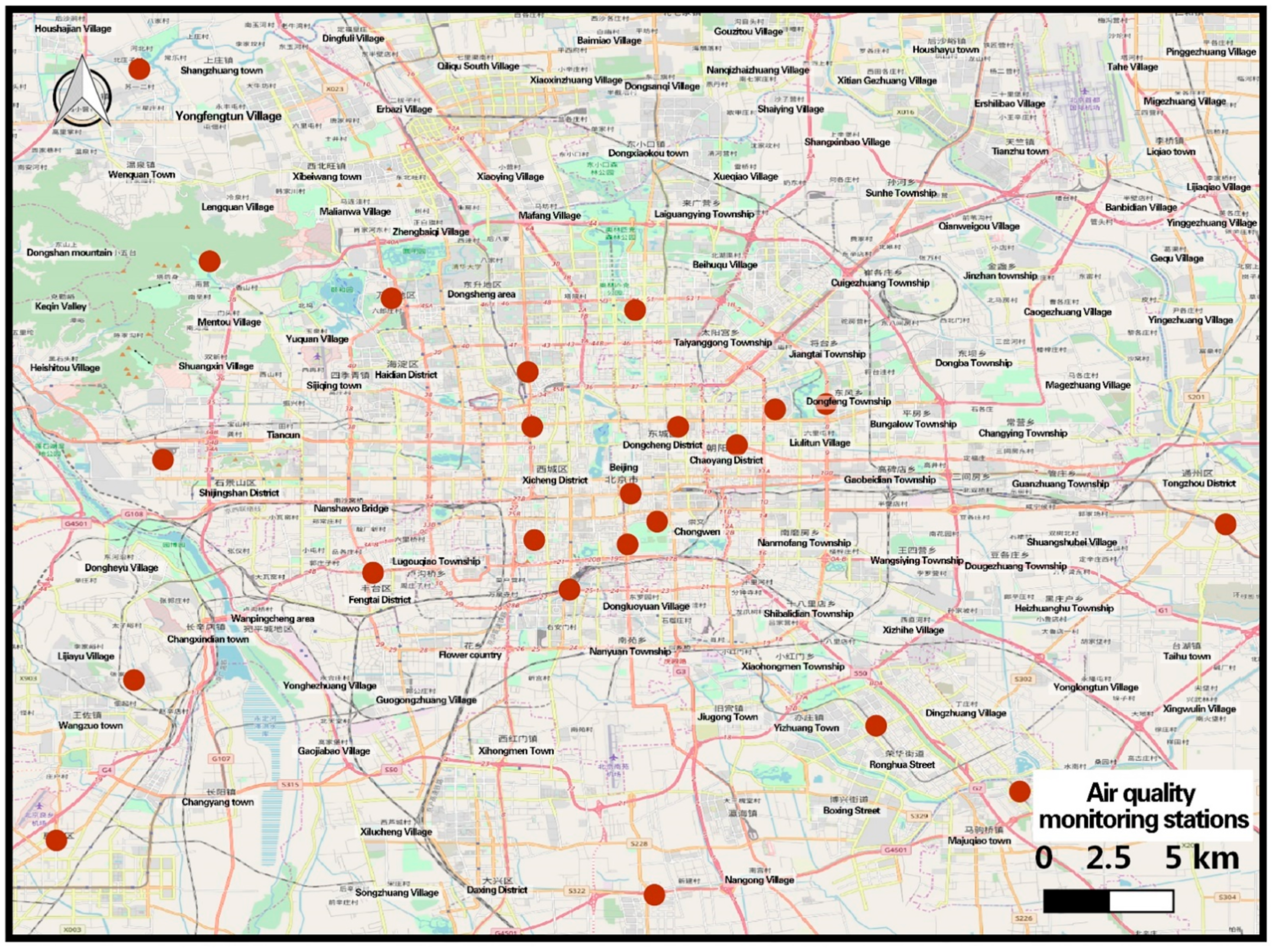
• The air quality monitoring data, which span the time period from 28 February 2013 to 28 February 2014 with a time granularity of one hour, were collected by the air quality monitoring stations in Beijing. The data include the monitoring station ID, monitoring station name, longitude and latitude, collection time, PM2.5 index, PM10 index, NO₂ index, and so on, where PM2.5 is the estimation target of this study model (As shown in Figure 1). And PM2.5 index, PM10 index, and NO₂ index are calculated by hourly average values.
• For meteorological monitoring data, the data span the time period from 28 February 2013 to 28 February 2014, with a time granularity of one hour. The data include information on temperature (°C), pressure (hPa), humidity (%), wind speed (km/h), wind direction (°), and description of weather conditions (rain, snow, clear, etc.). Temperature, pressure, humidity, and wind speed are calculated by hourly average values. Because the urban environmental protection department in the construction of air quality monitoring stations, will be equipped with meteorological characteristics monitoring equipment. Therefore, the meteorological Monitoring site is consistent with the air quality monitoring site.
• The vehicle track data, which are the location data recorded by the vehicle GPS of the cab, span from 1 May 2013 to 31 July 2013 with a time granularity of 10 s. The data include the vehicle number, UTC time, geographic coordinates (longitude, latitude), direction (unit: degree), speed (unit: m/s), passenger status (0/1), and other information, containing 3500 cab travel routes covering Beijing. The information was available for all areas of Beijing. The higher the traffic congestion level was, the higher the tailpipe emissions [36,37]. We calculated the traffic congestion level to estimate the impact of tailpipe emissions on air quality. The calculation of the traffic congestion factor is based on the traffic congestion evaluation method adopted by the Beijing Municipal Administration 2011 of Quality and Technical Supervision in 2009 [38].
• Urban road network, including vector layers of national roads, provincial roads, urban roads, urban ramps, line roads, and rural roads in Beijing.
• POI data record the distribution of geographic entities in urban space and can accurately reflect local urban spatial functions and social activity attributes. The data were derived from the Baidu Map API, totaling 380,000 POI points in Beijing, including geographic coordinates (longitude and latitude), names, detailed street addresses, and other information. The data were rendered by density to generate a POI density distribution map of Beijing. The urban POI data provide the distribution of different kinds of geographic entities in urban space, which is highly correlated with social activities and can reflect the distribution of people’s activities and the pattern of urban spatial functions.
• The land use type data were derived from the FROM-GLC-seg global land use raster image (available online: http://data.ess.tsinghua.edu.cn/ (accessed on 1 December 2019)) produced by the Earth System Science Research Center of Tsinghua University with a resolution of 30 m × 30 m, including farmland, forest, grassland, shrub, water body, human-made surface, bare land, and other types. Land use data reflect forest, shrub, and other vegetation types. This information has an important impact on air quality.
• Remote sensing image data were derived from the remote sensing satellite images of Google Maps. The data are from the 2013 Beijing remote sensing image, and the resolution is 30 m × 30 m. Remote sensing data can reflect forest, shrub, and other vegetation coverage. This information has an important impact on air quality.

In addition, the study area is located in northern China, climate change in the region shows distinctive temporal characteristics, and the meteorological environment shows a cyclical nature. Urban social activities have a high-temporal regularity. To determine the influence of periodicity and regularity on air quality, we labeled the season (1–4), week (1–7), and time period (0–23) to which each point in the experiment belonged and included them as influencing factors in the model.

2.2. Spatio-Temporal Data Preprocessing

The multisource data involved in this study have different spatial organization structures (point data, line data, and surface data), different spatio-temporal states (static data and dynamic data), different layer types (raster data and vector data), etc. If these data need to be fused and mined to reflect the same phenomenon and comprehensive spatio-temporal characteristics, a series of preprocessing work needs to be completed: (1) spatial unit setting, setting the way of dividing spatial units and the scale of dividing according to the demand for refinement of research content; (2) spatio-temporal data normalization processing, unifying the geospatial of vector data, raster data, and dynamic data, and preprocessing operations such as normalization and standardization of data; and (3) spatio-temporal feature scanning and extracting and fusing temporal and spatial features to avoid the information fragmentation of time and space.

(1)

Space unit setting

The division of spatial units is usually divided into homogeneous grid divisions or homogeneous functional area divisions (such as parcels and traffic districts). Considering that grid division can take into account the dynamic changes in the boundary, this paper adopts the homogeneous grid division method. For urban air quality, the grid scale is set to 1 km × 1 km, which can compensate for the influence of spatial inhomogeneity and meet the requirements of fine monitoring; therefore, the scale chosen in this paper is 1 km × 1 km. We divide the study area into a homogeneous grid, and after the division, we obtain a two-dimensional grid of 45 × 48, totaling 2160 grid cells, each of which represents a basic analysis unit, i.e., the target location to be predicted. The spatial data involved in this study are mapped onto the 2D grid according to the spatial location information.

(2)

Spatio-temporal data normalization

The spatio-temporal data normalization operation mainly includes 6 items: (1) interpolation of point data, where meteorological data are collected from meteorological monitoring stations as discrete point data; (2) we use inverse distance weighting (IDW) which is a kind of spatial interpolation method to obtain data for the whole study area; (3) resampling of raster data, as different spatial resolutions of raster data (land use type data) can be used to unify the resolution; (4) spatio-temporal fusion of dynamic data (vehicle trajectory data), for each moment to create a geospatial dataset, mapping the location information of each vehicle under that moment to the geospatial dataset; (5) normalization of continuous data (pollutant gas emission data, normalized and standardized to achieve uniformity in data magnitude) and discrete data (seasonal information, classified according to the categories of spring, summer, autumn, and winter).

(3)

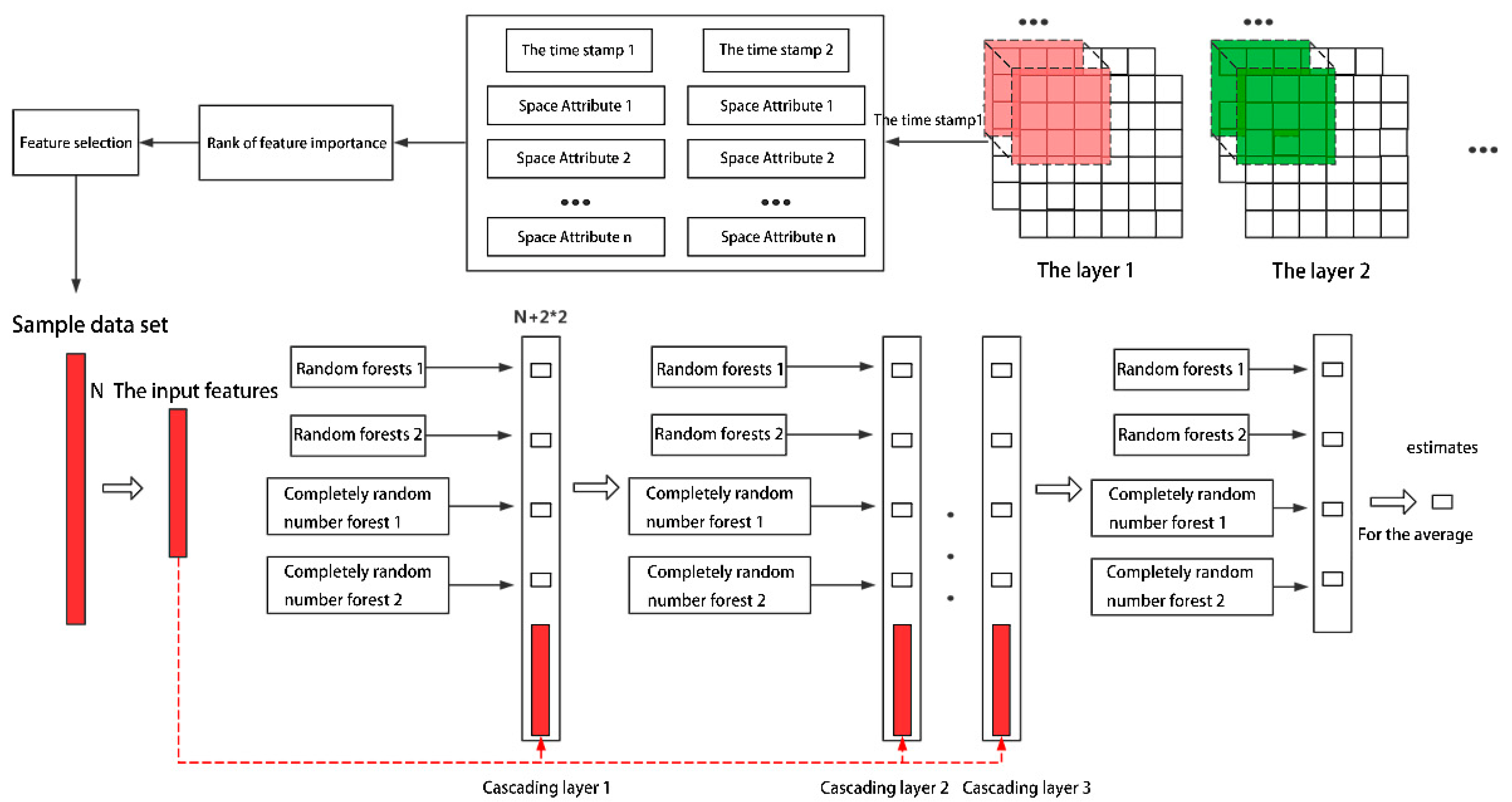
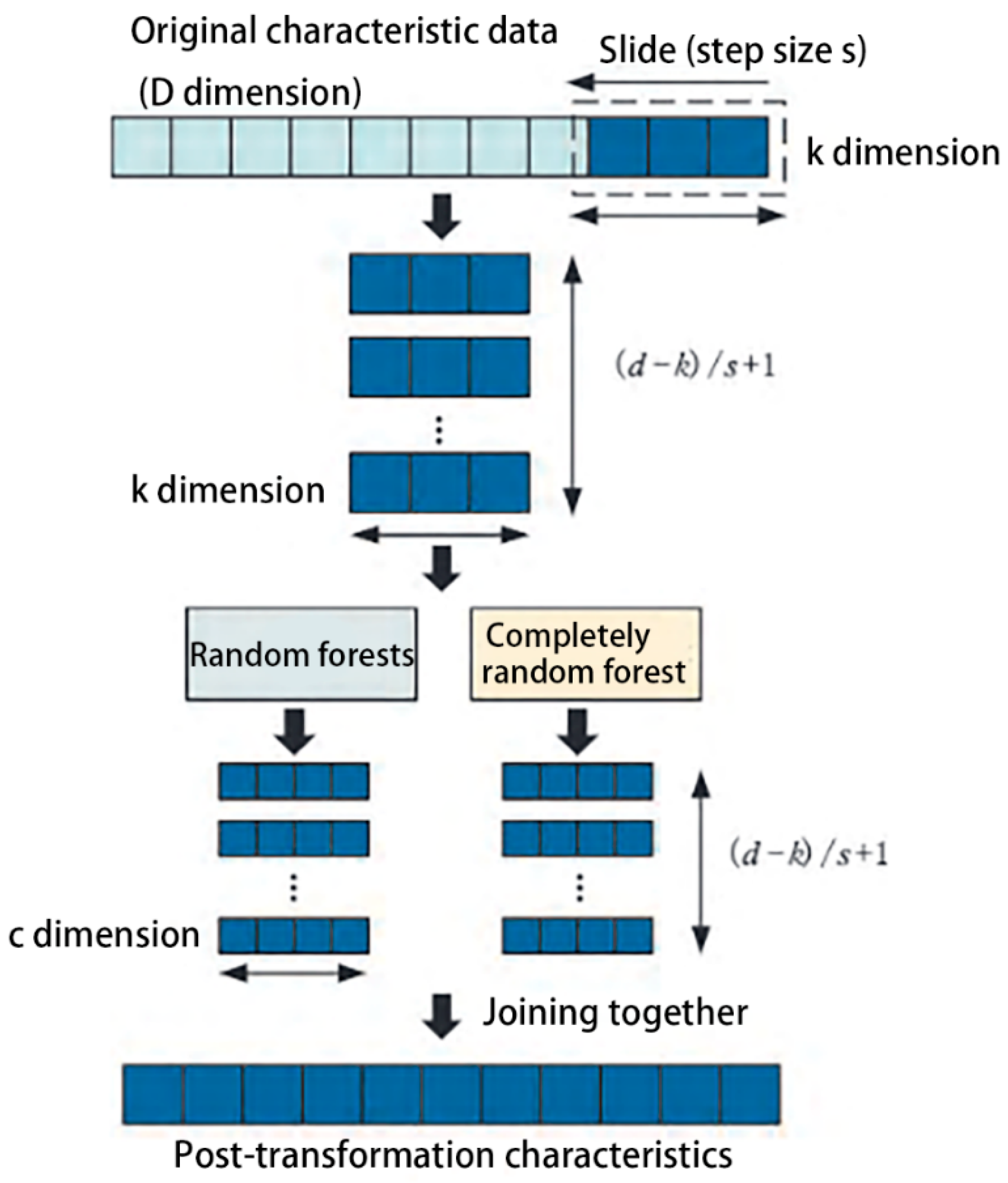
Spatio-temporal feature scanning model

Many existing air quality estimation methods are to extract spatio-temporal features by extracting temporal features and spatial features separately; however, this method cuts the connection between temporal and spatial attributes. To address this problem, this paper proposes a feature extraction model based on spatio-temporal integration, in which temporal and spatial features are extracted separately first, and then feature fusion is performed to establish spatio-temporal connections (as shown in Figure 2) to ensure that no spatio-temporal information is lost. First, during time feature extraction, time features of the current moment and the first $k$ moments are extracted by a time sliding window to obtain time series (Figure 2A):

$$t_{feature}=\left\{a_1\dots \dots a_{k-1},a_k\right\}$$

(1)

$a_k$ is the value of a position ($m,n$) at time $k$.

Secondly, based on the spatial autocorrelation theory, the spatial features are extracted, and at some position in time ($k$), the spatial features of the unit and its neighborhood are obtained by scanning the location information and its domain (Figure 2B):

$$s_{feature}=\left\{\begin{array}{c}{a}_{m-1,n-1},a_{m-1,n},a_{m-1,n+1}\\ a_{m,n-1},a_{m,n},a_{m,n+1} \\ a_{m+1,n-1},a_{m+1,n},a_{m+1,n+1}\end{array}\right\}$$

(2)

Finally, combining temporal and spatial features (Figure 2C).

$$Fusio{n}_{k,m,n}=\left\{{\left\{\begin{array}{c}{a}_{m-1,n-1},a_{m-1,n},a_{m-1,n+1}\\ a_{m,n-1},a_{m,n},a_{m,n+1} \\ a_{m+1,n-1},a_{m+1,n},a_{m+1,n+1}\end{array}\right\}}_1\dots \dots {\left\{\begin{array}{c}{a}_{m-1,n-1},a_{m-1,n},a_{m-1,n+1}\\ a_{m,n-1},a_{m,n},a_{m,n+1} \\ a_{m+1,n-1},a_{m+1,n},a_{m+1,n+1}\end{array}\right\}}_k\right\}$$

(3)

The above mainly focuses on dynamic data, while for static data, i.e., data without temporal attributes, only spatial feature extraction is performed in this paper.

In addition, the temporal sliding window size is chosen as moments t and (t + 1) due to the strongest correlation between the proximity moments; the size of the neighborhood sliding window is 3 km × 3 km, because the 1 km × 1 km grid is the minimum granularity required by the current refined estimation. It should be noted that the window size here is not fixed and can be chosen flexibly according to need.

We used the spatio-temporal feature scanning model to scan the features of the study area. The 129 total spatio-temporal features obtained after scanning are shown in

Table 1. Spatial and temporal characteristics related to air quality.

Features	Description	Number of Features
Time Factor	Hours, seasons, days of the week	3
Previous AQI	AQI of PM2.5 in the last hour	1
Meteorological characteristics of the current moment	Temperature (°C), pressure (hPa), humidity (%), and wind speed (km/h)	4
Meteorological characteristics of the previous moment	Temperature (°C), pressure (hPa), humidity (%), and wind speed (km/h)	4
Traffic Congestion Factor	Current hour and previous hour spatial 3 × 3 neighbourhood congestion level	2 × 9
POI Category	Number of each POI category in the spatial 3 × 3 neighbourhood	5 × 9
Surface vegetation type	Number of each vegetation type in the spatial 3 × 3 neighbourhood	6 × 9

. After extracting all spatio-temporal features, we constructed a sample dataset between the spatio-temporal features and PM2.5 indicators, and after data cleaning, we obtained a total of more than 86,000 valid data points and then divided the training set and test set according to a ratio of 7:3.

2.3. A Refined Urban Air Quality Estimation Method Integrating Multisource Spatio-Temporal Data

The method of urban air quality refinement estimation by fusing multisource spatio-temporal data is a method to accomplish deep relationship mining between urban spatio-temporal characteristics and PM2.5 indicators for urban air quality estimation by using a multigrained cascade forest algorithm.

To effectively realize spatio-temporal data mining, we design a refined urban air quality estimation process by fusing multisource spatio-temporal data. First, we use the feature scanning model based on spatio-temporal integration to scan different attribute layers that have completed spatio-temporal mapping, complete the fusion and association of temporal-spatial attributes, extract the air quality impact factors, complete the screening of impact factors according to the feature importance ranking, correlate the screened impact factors with the air quality indices to be estimated and build a sample dataset, perform the training set and test set based on the sample dataset. Finally, the cascade forest model is used to complete the training of the estimation model (as shown in Figure 3).

(1)

Feature Screening

In the process of model training, information redundancy will affect the model training accuracy. Therefore, feature screening is an essential part. The selection of a reasonable number of features depends on the importance of each feature in the model, and the measure of importance, in turn, depends on the magnitude of the contribution of the feature. In random forests, when solving regression problems, the method of ranking the importance of features usually uses MSE (mean square error) [39,40]. Therefore, in this paper, we choose to use MSE as a judgment indicator to rank the spatio-temporal features obtained from the feature scanning model, and the results show that the temporal factor and meteorological factor are much more important than the traffic congestion factor, POI category, and surface vegetation type. Such ranking results are also basically in line with our expectation that air quality is highly dependent on the influence of temporal regularity and meteorological conditions. On the other hand, the three lower ranked features also weaken the amount of information they contain due to the increased number of features after spatial sliding window traversal. Therefore, in this paper, the three lower-ranked features are further processed, as shown in

Table 2. Spatial and temporal characteristics of air quality after screening.

Features	Description	Number of Features
Time Factor	Hours, seasons, days of the week	3
Previous AQI	AQI of PM2.5 in the last hour	1
Current moment meteorological characteristics	Temperature (°C), pressure (hPa), humidity (%), and wind speed (km/h)	4
Meteorological characteristics of the previous moment	Temperature (°C), pressure (hPa), humidity (%), and wind speed (km/h)	4
Traffic Congestion Factor	Current hour and previous hour spatial 3 × 3 neighbourhood congestion averages	2
POI Category	Average of the number of POI categories in the current and previous hour spatial 3 × 3 neighbourhoods	5
Surface vegetation type	Mean values of the number of vegetation types in each spatial 3 × 3 neighbourhood at the current hour and the previous hour	6

. The original 9 neighborhood features are averaged, and the number of features is reduced from the original 9 to 1. This not only preserves the information of the features in this category but also reduces the number of features to avoid the dispersion of information, and the subsequent training results also prove that such a processing method is better than unprocessed or direct rejection.

The sample dataset is processed by feature filtering, and the number of samples in the new sample dataset remains unchanged, except that the number of 129 spatio-temporal features is reduced to 25 to reduce the redundancy of information. Similarly, the spatio-temporal features in the training and test sets are also changed accordingly, and the new training dataset formed after feature filtering will be placed into the subsequent cascade forest model for training and calibration, and the model estimation and visualization will then be completed.

(2)

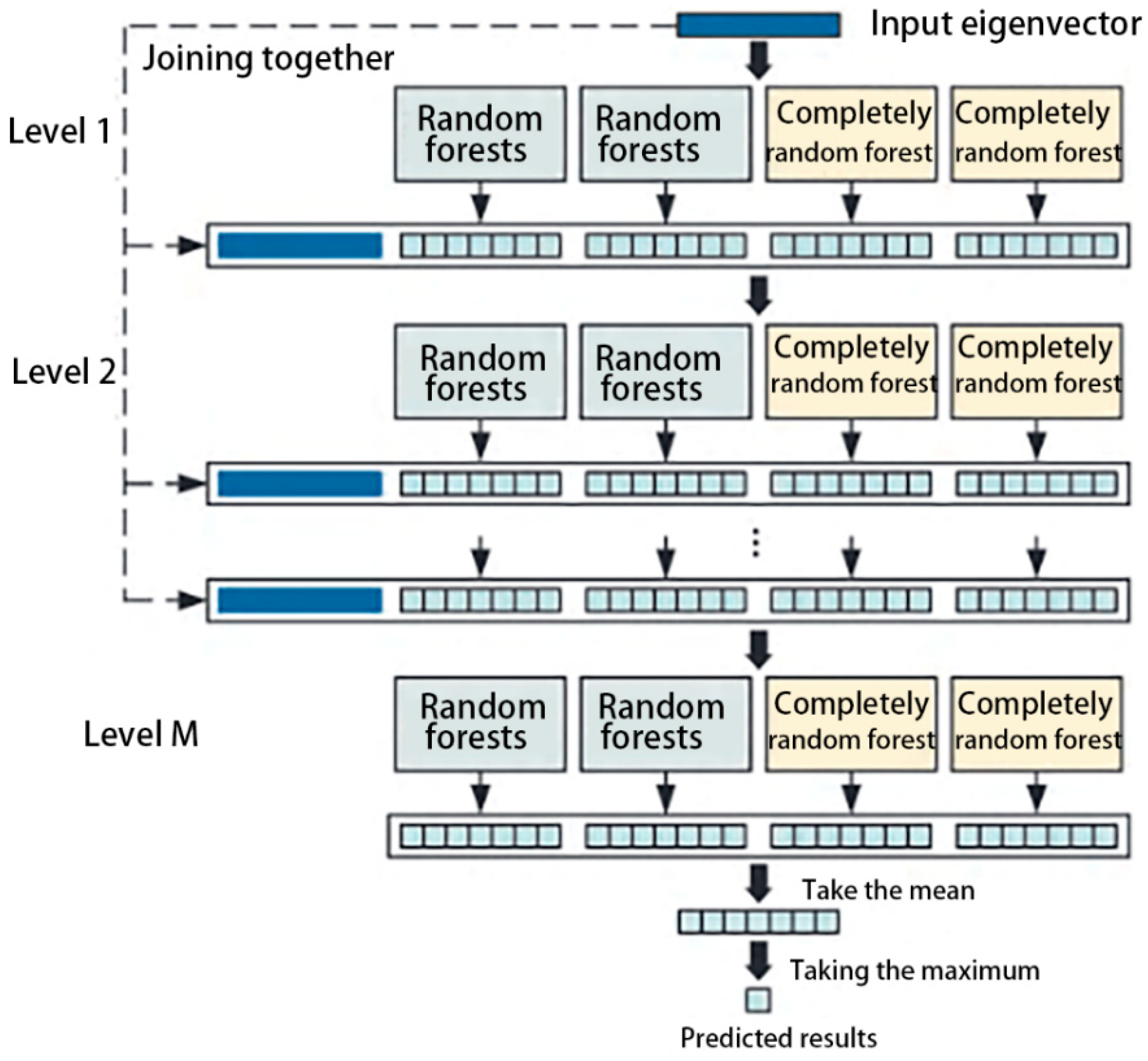
Multigrained cascade forest algorithm

The multigrained cascade forest approach [41] is a machine learning method based on a random forest [42]. The most important feature of this method is that it can achieve adaptive model parameters without relying on human experience, the training difficulty is low, and it can effectively explore the sequential information of sequence data and the spatial correlation information of spatial data.

The multigrained cascade forest model mainly consists of two parts: the multigrained scan structure and the cascade forest structure. The multigrained scan structure uses multiple windows of different widths for slide sampling to obtain multiple interconnected and differentiated subsamples. The subsamples are trained with the ordinary random forest classifier and the complete random forest classifier, and the output category probability vectors are stitched to obtain the final transformation features, as shown in Figure 4.

The whole feature scanning transformation process is introduced by using a sliding window of width k dimensions as an example. When the initial input eigenvector is d-dimension, and the sliding step is s, the number of samples is m = (d − k)/s + 1. The sample set is obtained by Formulas (4)–(6).

$$Data=\left\{a_1,a_2,\dots \dots a_d\right\};$$

(4)

$$Window=\left\{b_1,b_2,\dots \dots b_m\right\}=\left\{\begin{array}{c}1, 0, 0\dots \dots 0\\ 1,1,0\dots \dots 0\\ \dots \dots \\ 0,0,0\dots \dots 1\end{array}\right\} ;$$

(5)

$$Sample=Dat{a}_{original}\times Window=\left\{\left\{a_1,a_2,\dots \dots a_d\right\}{b}_1,\left\{a_1,a_2,\dots \dots a_d\right\}{b}_2,\dots \dots \left\{a_1,a_2,\dots \dots a_d\right\}{b}_m\right\};$$

(6)

where the number of 1 s in $b$ is k, and the number of 0 s before 1 is s.

The samples are trained with two classifiers (ordinary random forest (ORF) and completely random forest (CRF)). After training, each classifier gets a c-dimensional probability vector (c is the number of categories set in advance), which represents the probability that a sample falls into each category. Finally, the two classifiers output a total of 2 × m probability vectors. The 2 × m × c-dimensional transformed feature vectors are obtained by stitching all obtained category probability vectors (Formula (7)).

$$Featur{e}_{2\times m\times n}=\left\{{\left\{Ou{t}_{ORF}\right\}}_{m\times n},{\left\{Ou{t}_{CRF}\right\}}_{m\times n}\right\};$$

(7)

The multigrained cascade forest model uses a hierarchical structure, that is, the output of the previous forests serves as the input of the next forests, as shown in Figure 5. The output of the last layer of forest (2 m probability vectors) is averaged to obtain a probability vector. Finally, the smallest value of the vector is used as the predicted value.

Two different forest classifiers in each layer increase the diversity of model integration. Multiple forest classifiers can make full use of the differences in features, which is conducive to the mining of feature information. To avoid the occurrence of overfitting, k-fold cross-validation is used in the training process of each forest classifier in each layer of the cascaded forest structure.

(3)

Model calibration and implementation

a.

Model parameter calibration

After the training of the urban air quality estimation model, further calibration of the model is needed to further improve the estimation accuracy. The parameters that can be adjusted in the cascade forest include the following: (1) the maximum number of features involved in attribute classification; while the traditional decision tree selects the best attribute in the current node attribute set (assuming there are n attributes) for attribute classification, the random forest selects the best attribute in the random attribute set by randomly selecting k sub-attributes from the set of n attributes; the parameter k controls the degree of randomness in attribute partitioning; (2) the number of base learners and the number of decision trees contained in the cascade forest; the number of forests and the number of trees contained in the forest jointly determine the complexity and training effect of the model; and (3) the number of cascade layers, which also determines the training effect and time complexity of the model. We optimized the model parameters through experiments and tests.

• b.

  Algorithm implementation

Our experiments are based on the cascade forest source code (available online: https://github.com/kingfengji/gcForest (accessed on 1 February 2021)). For feature filtering, model correction methods, and related model implementation, we draw on the Numpy, Pandas, and Scikit-learn libraries based on the Python 3.5 libraries (available online: https://www.python.org/ (accessed on 5 September 2020)) which was originally developed by Guido van Rossum in the late eighties and early nineties at the National Research Institute for Mathematics and Computer Science in the Netherlands.

3. Results

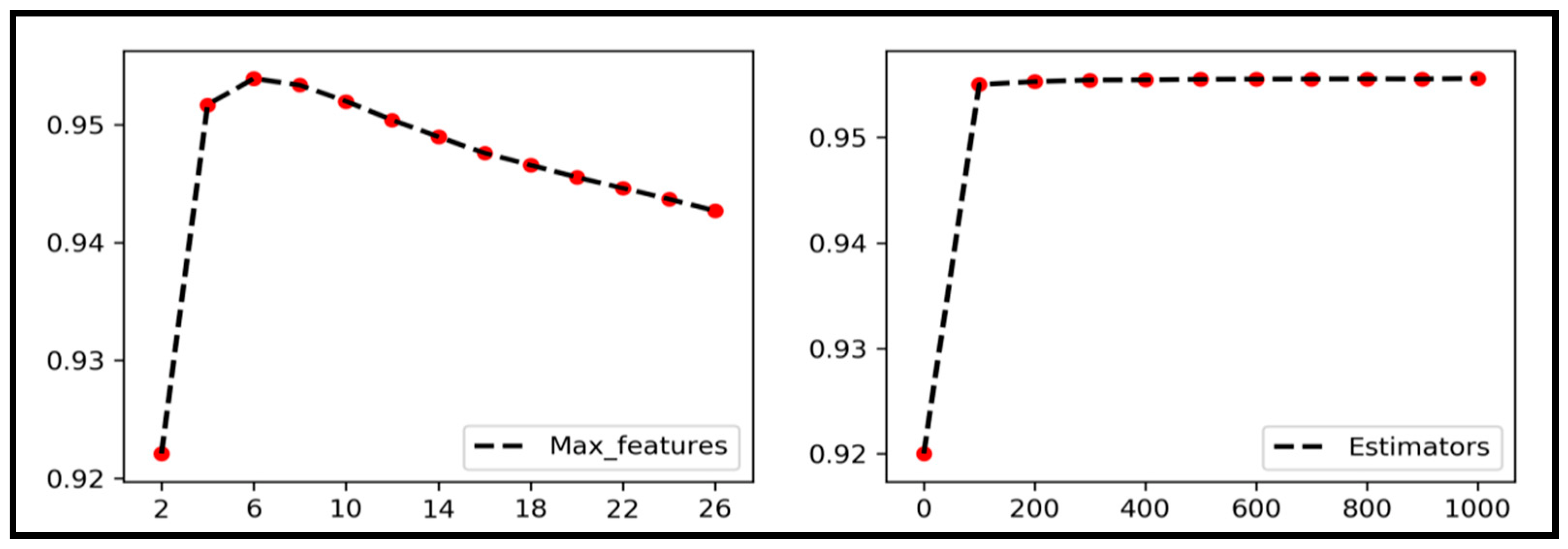
3.1. Parameter Optimization Results

After several model experiments and tests, the following model parameters are corrected in this paper.

(1)

Maximum number of features involved in judgement when dividing attributes (m)

In the usual random forest model setting, assuming that the full set of attributes contains a total of s attributes, the default setting of m is generally s or $\sqrt{s}$. To better judge the relationship between this parameter and the training effect, we tested the relationship between the value of m and the accuracy several times. The test results are shown on the left of Figure 6, where the horizontal axis represents the maximum number of features m involved in the judgment when dividing attributes, and the vertical axis represents the fitting accuracy. From the test results, we can see that the fitting accuracy reaches the critical point when m is taken as six; therefore, we set this parameter as six.

(2)

Number of base learners and the number of decision trees they contain (k)

The default number of base learners for the cascaded forest model is four, which includes two random forests and two completely random tree forests. After testing, this default structure is retained for the number of base learners. The number of trees included in each base learner is still tested with different parameters in this paper. As shown in Figure 6, the horizontal axis represents the number of trees, and the vertical axis represents the fitting accuracy. The results show that the fitting accuracy of the model tends to be stable when k is taken 100 above and reaches the highest value at approximately 300. However, considering that the value of k can have a serious impact on the time complexity of model training, 100 is still chosen as the final value of this parameter in this paper.

(3)

Number of cascade layers (n)

In general, the setting of the number of cascade layers (n) depends on the training efficiency of the model, and when the training accuracy of four successive layers no longer improves, the cascade is stopped, and the structure of the current optimal training result is saved as the trained model. Similarly, such a strategy is adopted in the experiments described in this paper, and the value of n is finally determined as four layers.

3.2. Model Performance Evaluation

In this paper, the model training results were evaluated and compared, the evaluation method adopted was 10-fold-cross validation, and the evaluation metric was chosen as the goodness-of-fit (R²). The evaluation results show that the results of the evaluation metric R² value are close to nearly one, such that the training results indicate that the model learns the information contained in the input features. To verify the generalization ability of the model, we use the test dataset to validate the trained model. The evaluation metrics are selected as the goodness of fit (R²) and the root mean square error (RMSE), and the test results are 0.961 and 17.47, respectively.

This experiment was also compared with other machine learning algorithms based on the same data, and the comparison algorithms chosen were the more widely used neural network (ANN) and random forest (RF). The structure of the neural network is chosen as three layers, which contain one hidden layer. The neuron structure of each layer is 25 × 40 × 1, the activation function of the hidden layer is chosen as the ReLU function, the activation function of the output layer is the linear function, the training algorithm is Rmsprop, and the loss function is the mean squared difference function. The parameters of the random forest are chosen to be consistent with the base learner used in the experimental part of this paper. These two algorithms are compared with the model used in this paper (CF) in terms of training results, testing results, and mean squared deviation. The comparison results are shown in

Table 3. Comparison results of different algorithms.

Algorithm	R_CV2	R2_Test	RMSE
ANN	0.931	0.934	23.01
RF	0.993	0.955	18.96
CF	0.999	0.961	17.47

, and it can be seen that the model described in this paper shows better performance according to all kinds of evaluation indices, which validates the reasonable scientific design of the algorithm framework reported in this paper.

In addition to comparing similar algorithms, this experiment also compares the accuracy of the PM2.5 estimation model (FFA) proposed by Dr. ZhengYu of Microsoft Research [34]. The FFA model models temporal and spatial attributes in different ways and couples the two in a co-training manner to build a PM2.5 estimation model. In this paper, the accuracy of the model used is compared with that of the FFA model on the same dataset, and the accuracy indicators p (Equation (8)) and error e (Equation (9)) used in the FFA model are selected for comparison. The comparison results are shown in

Table 4. Comparison results of different models.

Models	p	e
FFA	0.749	23.7
CF	0.926	10.1

. The experimental results of this paper outperform the FFA model in different metrics, which also verifies the superiority of the feature scanning method and the model training method used in this paper.

$$p=1-\frac{{\sum }_i\left|\widehat{y_i}-y_i\right|}{{\sum }_i{y}_i}$$

(8)

$$e=\frac{{\sum }_i\left|\widehat{y_i}-y_i\right|}{n}$$

(9)

where p represents the estimation accuracy, e represents the estimation error, n represents the number of datasets to be estimated, $y_i$ is the actual label value of the ith data, and $y_i$ is the estimated value of the ith data.

In addition, it is difficult to validate the model estimates due to the lack of real PM2.5 data for areas other than one monitoring station when making global estimates for the study area. For this reason, we randomly selected data for multiple weeks (seven days × 24 h), randomly excluded two air quality monitoring stations in each estimation period, and interpolated the remaining 20 air quality monitoring stations to obtain the meteorological data of other non-monitoring stations in the spatial grid. The trained model was then used to estimate the PM2.5 values for the entire study area in the current time period, and the results of the grid where the excluded stations were located were extracted for each time period and compared with the real values to measure the generalization performance of the model.

As shown in Figure 7, the data from three weeks were randomly extracted in this paper, and a total of 590 valid time periods were obtained, excluding some missing moments. By randomly eliminating two stations, the station IDs were chosen as 1012 (red) and 1014 (blue). For each time period, the data of the 20 stations other than the excluded stations were interpolated to obtain the meteorological data of other locations, and then the trained model was used to estimate them. After comparing the estimated values with the true values of the excluded grid at each time, the fitted results at the extraction time were 0.826 and 0.936, respectively. Among them, the fitted results for Station 1012 were slightly lower. After further analysis, it was found that Station 1014 (blue) was located in the center of the interpolation region, while the excluded Station 1012 (red) was at the boundary of the interpolation region, as shown in Figure 7. This was due to the degree of coverage of meteorological data and the boundary effect of the interpolation method in which the accuracy of the estimation results fluctuated from the center to the boundary, which is a drawback that is difficult to avoid in the current study [43]. However, this also proves the stability of the estimation model in this paper; even with the boundary effect caused by the interpolation, the model can still achieve high fitting accuracy.

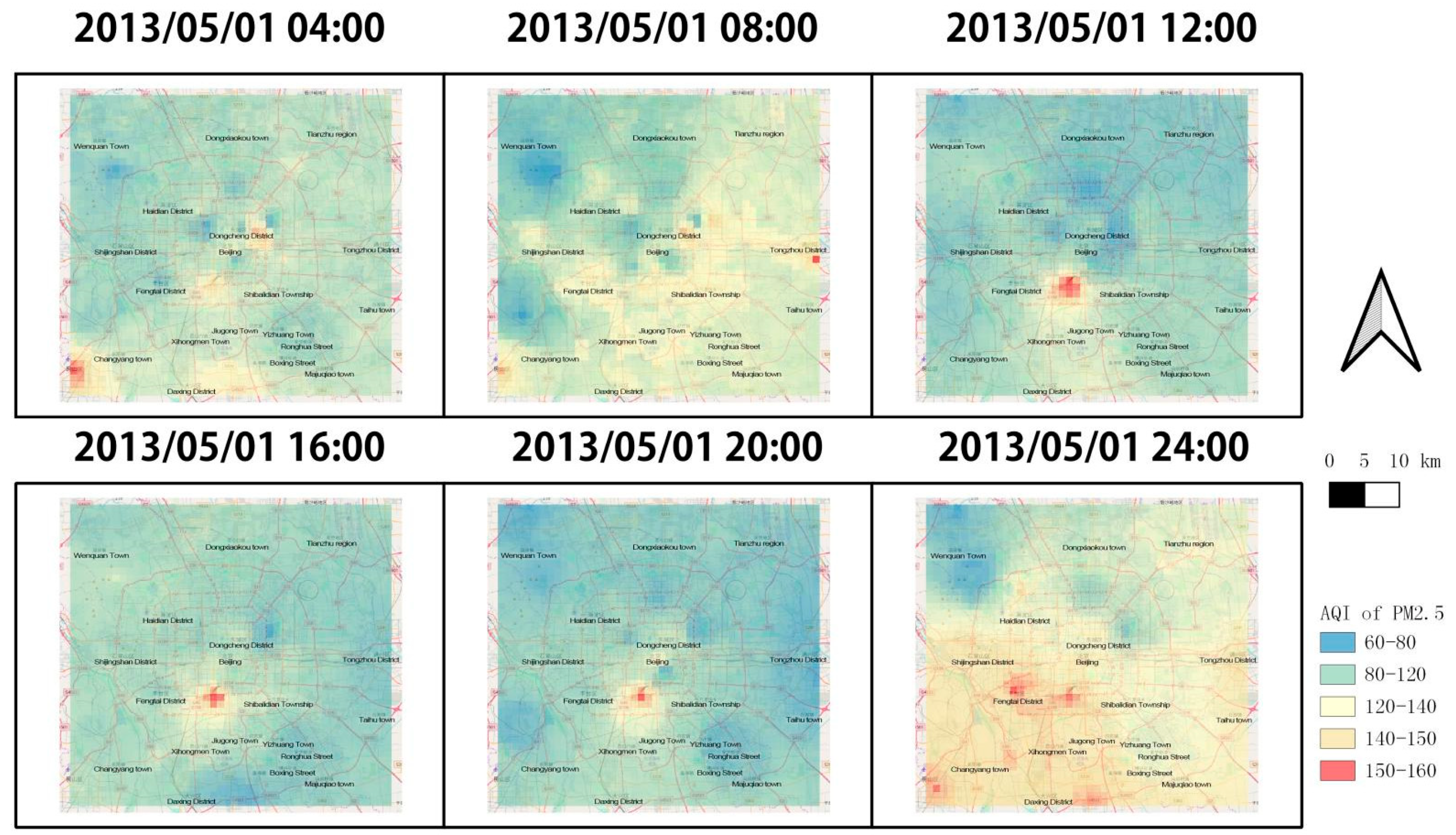
3.3. Real-Time Estimation of Effects

The PM2.5 estimation and the visualization of the results were carried out for all time periods (1:00 am to late at night at 12:00 pm) on the day of 1 May 2013 (shown in Figure 8). From the estimation results, we can see that the cascade forest-based real-time urban air quality estimation model with fine-temporal and spatial granularity proposed in this part of the experiment had a good estimation effect, and the visualization results had a smooth transition and could clearly show the air differences in microregions. From the estimation results of the day, it can be seen that the air quality was better in the afternoon to evening hours than in the early morning to morning hours, and the air pollution situation was consistent with the previous research findings, showing an intensive pollution pattern [17]. Severe pollution areas in the first half of the day period were mainly found in Chongwenmen, Xuanwumen, Haidian, Daxing, Yizhuang, Shijingshan, and other areas, while the air quality in the second half of the day period formed a peak pollution area in Fengtai District.

In terms of the distribution pattern of air pollution, the overall air quality in Beijing was high in the south and low in the north and high in the east, and low in the west on 1 January 2013. Among them, especially in the southwest, the whole-day air quality in the same time ranking was in the serious pollution area, and the areas included Fengtai District and Fangshan District. The central part of the city as a whole had an intermediate level of pollution, but considering the large population living in the city, the pollution level was intermediate, but the AQI was still high between 100 and 200 in the orange warning of “unhealthy for sensitive people” and “unhealthy”. In the long run, this will cause great harm to the health of the residents. The northern part of the country is in a better position overall in terms of air quality due to its dense vegetation and proximity to natural entities such as forest parks and reservoirs. Therefore, in general, Labour Day in 2013 was a popular holiday, and there was a large number of traveling residents and foreign tourists; however, the overall air quality situation in Beijing is still not optimistic and is at a level that threatens human health.

The government and related departments in 2013 promoted industrial optimization, clean energy, travel restrictions, and other energy saving and emission reduction projects, which aim to gradually improve the overall air quality environment in Beijing. The air quality estimation model proposed in this paper will provide contribute to air environmental management based on its excellent performance and estimation effect.

4. Discussion

In this study, by fusing urban multisource spatio-temporal data, we accomplish the filling of gaps in spatio-temporal fine-scale urban air quality information and realize fine-scale air quality estimation at a microscale. This method uses a spatio-temporal integrated feature scanning model to effectively extract the spatio-temporal features of urban big data and then completes the real-time urban air quality estimation at a fine scale (1 km × 1 km or below) by using the cascade forest algorithm. Through model evaluation tests, the estimation model performs well in terms of generalization ability and accuracy, and the model performance is better compared with other machine learning methods.

Previous studies [44,45] on air quality estimation based on data fusion have shown that spatio-temporal high-resolution estimation can be achieved via data fusion, and the average of its goodness-of-fit (R²) was approximately 0.9. In this study, the goodness-of-fit (R²) and root mean square error (RMSE) of the air quality estimation model are 0.961 by fusing urban multisource data that can reflect social activities.

By fusing urban multisource data containing social activity information and mining social activity information closely related to air quality, this study supplements air quality information in site-free areas to compensate for the lack of urban air quality monitoring capacity; by constructing a refined urban air quality estimation model with integrated temporal, spatial, and attribute characteristics, the granularity of the perceived spatial differences in urban air quality is improved. Moreover, this study further verifies the effectiveness of data fusion methods for air quality estimation and provides ideas for effective data selection in the process of data fusion.

There are also shortcomings of this study. The meteorological data of areas without monitoring stations are obtained by interpolation methods, which affects the fitting accuracy of the estimation model. However, at the current stage, there is a lack of good solutions for this problem. If meteorological monitoring devices are widely available and sensor networks can cover a large area, this will provide us with a better solution for improving the fitting accuracy [46,47,48,49].

In our future research, we will further study the refined air quality estimation, including focusing on street-level air quality estimation, detecting air quality changes within the local urban space, and conducting research on the linkage between urban air quality, social activities of people, and urban internal functions to better provide reliable reference information and guidance for urban environmental decision-making and management.

5. Conclusions

With the development of machine learning and big data analysis technology, there is a trend of using data fusion technology to achieve refined urban air quality estimation. The current data fusion method still suffers from the fragmentation of the three dimensions of time, space, and attributes, which can lead to the accumulation of errors in the modeling process, and the estimation results do not conform to the geographic phenomena and patterns. At the same time, data fusion mainly focuses on the fusion of the same attribute data at different resolutions, and this approach does not consider the influence of social activities on air quality, which leads to an inability to detect air quality differences in a small area.

Based on the above problems, this study proposes a fine-scale urban air quality estimation method integrating multisource spatio-temporal data. The method realizes 3D comprehensive feature extraction of time, space, and attributes. A fine-scale urban air quality estimation model is constructed by using the cascade forest algorithm to achieve high spatial and temporal resolution urban air quality estimation. At the same time, this method introduces social activity data to improve the effect of air quality estimation, which provides a new idea for improving the ability of information mining.

In the future, we will also consider the relationship between air circulation, wind speed, and social activities of people and urban functions. Because these relationships reflect information on harmful gas emissions and flows, this information can help to trace the sources and flow paths of harmful gas emissions, which will further help to refine spatial quality estimation and prediction.

References

1. Greenbaum, D.S.; Bachmann, D.; Krewski, D.; Samet, J.M.; White, R.; Wyzga, R.E. Particulate Air Pollution Standards and Morbidity and Mortality: Case Study. Am. Ournal Epidemiol. 2001, 154 (Suppl. S12), S78–S90. [Google Scholar] [CrossRef] [PubMed] [Green Version]
2. Jiménez-Guerrero, P.; Pérez, C.; Jorba, O.; Baldasano, J.M. Contribution of Saharan dust in an integrated air quality system and its on-line assessment. Geophys. Res. Lett. 2008, 35, 183–199. [Google Scholar] [CrossRef] [Green Version]
3. Millman, A.; Tang, D.; Perera, F.P. Air pollution threatens the health of children in China. Pediatrics 2008, 122, 620–628. [Google Scholar] [CrossRef] [Green Version]
4. Arnold, R.; Dennis, R.L. Testing CMAQ chemistry sensitivities in base case and emissions control runs at SEARCH and SOS99 surface sites in the southeastern US. Atmos. Environ. 2006, 40, 5027–5040. [Google Scholar] [CrossRef]
5. Martin, R.V. Satellite Remote Sensing of Surface Air Quality. Atmos. Environ. 2008, 42, 7823–7843. [Google Scholar] [CrossRef]
6. Wu, L.; Bocquet, M. Optimal redistribution of the background ozone monitoring stations over France. Atmos. Environ. 2011, 45, 772–783. [Google Scholar] [CrossRef] [Green Version]
7. Austin, E.; Coull, B.A.; Zanobetti, A.; Koutrakis, P. A framework to spatially cluster air pollution monitoring sites in US based on the PM2.5 composition. Environ. Int. 2013, 59, 244–254. [Google Scholar] [CrossRef]
8. Goodsite, M.E.; Hertel, O.; Johnson, M.S.; Jørgensen, N.R. Urban air quality: Sources and concentrations. Air Pollut. Sources Stat. Health Eff. 2021, 193–214. [Google Scholar] [CrossRef]
9. Jorquera, H.; Montoya, L.D.; Rojas, N.Y. Urban air pollution. In Urban Climates in Latin America; Springer: Cham, Switzerland, 2019; pp. 137–165. [Google Scholar]
10. Seo, J.; Park, D.-S.R.; Kim, J.Y.; Youn, D. Effects of meteorology and emissions on urban air quality: A quantitative statistical approach to long-term records (1999–2016) in Seoul, South Korea. Atmos. Chem. Phys. 2018, 18, 16121–16137. [Google Scholar] [CrossRef] [Green Version]
11. Hsieh, H.P.; Lin, S.D.; Zheng, Y. Inferring Air Quality for Station Location Recommendation Based on Urban Big Data. In Proceedings of the 21th SIGKDD conference on Knowledge Discovery and Data Mining, Sydney, Australia, 10–13 August 2015; pp. 437–446. [Google Scholar]
12. Li, T.; Shen, H.; Zeng, C.; Yuan, Q.; Zhang, L. Point-surface fusion of station measurements and satellite observations for mapping PM2.5 distribution in China: Methods and assessment. Atmos. Environ. 2017, 152, 477–489. [Google Scholar] [CrossRef] [Green Version]
13. Gurram, S.; Stuart, A.L.; Pinjari, A.R. Agent-based modeling to estimate exposures to urban air pollution from transportation: Exposure disparities and impacts of high-resolution data. Comput. Environ. Urban Syst. 2019, 75, 22–34. [Google Scholar] [CrossRef]
14. Shad, R.; Mesgari, M.S.; Abkar, A.; Shad, A. Predicting air pollution using fuzzy genetic linear membership kriging in GIS. Comput. Environ. Urban Syst. 2009, 33, 472–481. [Google Scholar] [CrossRef]
15. Zou, B.; Pu, Q.; Bilal, M.; Weng, Q.; Zhai, L.; Nichol, J.E. High-Resolution Satellite Mapping of Fine Particulates Based on Geographically Weighted Regression. In IEEE Geoscience & Remote Sensing Letters; IEEE: Piscataway, NJ, USA, 2016; Volume 13, pp. 495–499. [Google Scholar]
16. You, W.; Zang, Z.; Zhang, L.; Li, Y.; Pan, X.; Wang, W. National-Scale Estimates of Ground-Level PM2.5 Concentration in China Using Geographically Weighted Regression Based on 3 km Resolution MODIS AOD. Remote Sens. 2016, 8, 184. [Google Scholar] [CrossRef] [Green Version]
17. Feizizadeh, B.; Blaschke, T. Examining urban heat island relations to land use and air pollution: Multiple endmember spectral mixture analysis for thermal remote sensing. IEEE J. Sel. Top. Appl. Earth Obs. Remote Sens. 2013, 6, 1749–1756. [Google Scholar] [CrossRef]
18. Hu, X.; Waller, L.A.; Lyapustin, A.; Wang, Y.; Al-Hamdan, M.Z.; Crosson, W.L.; Estes, M.G., Jr.; Estes, S.M.; Quattrochi, D.A.; Puttaswamy, S.J.; et al. Estimating ground-level PM2.5 concentrations in the Southeastern United States using MAIAC AOD retrievals and a two-stage model. Remote Sens. Environ. 2014, 140, 220–232. [Google Scholar] [CrossRef]
19. Lee, H.J.; Liu, Y.; Coull, B.A.; Schwartz, J.; Koutrakis, P. A novel calibration approach of MODIS AOD data to predict PM2.5 concentrations. Atmos. Chem. Phys. 2011, 11, 9769–9795. [Google Scholar] [CrossRef] [Green Version]
20. Han, W.; Ling, T.; Chen, Y. A new algorithm for aerosol retrieval using H-1 CCD and MODIS NDVI data over urban areas. In Proceedings of the Geoscience & Remote Sensing Symposium, Beijing, China, 10–15 July 2016. [Google Scholar]
21. Xiang, J.; Li, R.; Wang, G.; Qie, G.; Wang, Q.; Xu, L.; Zhang, M.; Tang, M. Modeling Urban PM2.5 Concentration by Combining Regression Models and Spectral Unmixing Analysis in a Region of East China. Water Air Soil Pollut. 2017, 228, 250. [Google Scholar] [CrossRef]
22. Huang, B.; Wu, B.; Barry, M. Geographically and Temporally Weighted Regression for Modeling Spatio-Temporal Variation in House Prices; Taylor & Francis, Inc.: Oxfordshire, UK, 2010; Volume 24, pp. 383–401. [Google Scholar]
23. Chu, H.J.; Huang, B.; Lin, C.Y. Modeling the spatio-temporal heterogeneity in the PM10-PM2.5 relationship. Atmos. Environ. 2015, 102, 176–182. [Google Scholar] [CrossRef]
24. He, Q.; Bo, H. Satellite-based mapping of daily high-resolution ground PM2.5 in China via space-time regression modeling. Remote Sens. Environ. 2018, 206, 72–83. [Google Scholar] [CrossRef]
25. Zou, B.; Chen, J.; Zhai, L.; Fang, X.; Zheng, Z. Satellite Based Mapping of Ground PM2.5 Concentration Using Generalized Additive Modeling. Remote Sens. 2016, 9, 1. [Google Scholar] [CrossRef] [Green Version]
26. Zou, B.; Zheng, Z.; Wan, N.; Qiu, Y.; Wilson, J.G. An optimized spatial proximity model for fine particulate matter air pollution exposure assessment in areas of sparse monitoring. Int. Ournal Geogr. Inf. Sci. 2015, 30, 727–747. [Google Scholar] [CrossRef]
27. Kovács, A.; Leelőssy, Á.; Tettamanti, T.; Esztergár-Kiss, D.; Mészáros, R.; Lagzi, I. Coupling traffic originated urban air pollution estimation with an atmospheric chemistry model. Urban Clim. 2021, 37, 100868. [Google Scholar] [CrossRef]
28. Harrison, R.M.; Van Vu, T.; Jafar, H.; Shi, Z. More mileage in reducing urban air pollution from road traffic. Environ. Int. 2021, 149, 106329. [Google Scholar] [CrossRef] [PubMed]
29. Borck, R.; Schrauth, P. Population density and urban air quality. Reg. Sci. Urban Econ. 2021, 86, 103596. [Google Scholar] [CrossRef]
30. Ma, Y.; Li, J.; Guo, R. Application of data fusion based on deep belief network in air quality monitoring. Procedia Comput. Sci. 2021, 183, 254–260. [Google Scholar] [CrossRef]
31. Yu, Z. Methodologies for Cross-Domain Data Fusion: An Overview. IEEE Trans. Big Data 2015, 1, 16–34. [Google Scholar]
32. Liu, J.; Li, T.; Xie, P.; Du, S.; Teng, F.; Yang, X. Urban big data fusion based on deep learning: An overview. Inf. Fusion 2020, 53, 123–133. [Google Scholar] [CrossRef]
33. Zheng, Y.; Yi, X.; Li, M.; Li, R.; Shan, Z.; Chang, E.; Li, T. Forecasting Fine-Grained Air Quality Based on Big Data: ACM SIGKDD International Conference on Knowledge Discovery and Data Mining. In Proceedings of the 21th ACM SIGKDD International Conference on Knowledge Discovery and Data Mining, Sydney, Australia, 10–13 August 2015. [Google Scholar]
34. Zheng, Y.; Chen, X.; Jin, Q.; Chen, Y.; Qu, X.; Liu, X.; Chang, E.; Ma, W.; Rui, Y.; Sun, W. A Cloud-Based Knowledge Discovery System for Monitoring Fine-Grained Air Quality. MSR-TR-2014-40. Tech. Rep.. 2014, Volume 1, p. 40. Available online: https://www.microsoft.com/en-us/research/wp-content/uploads/2016/02/UAir20Demo.pdf (accessed on 3 April 2022).
35. Zheng, Y.; Liu, F.; Hsieh, H.P. U-Air: When urban air quality inference meets big data: ACM SIGKDD International Conference on Knowledge Discovery and Data Mining. In Proceedings of the 19th SIGKDD conference on Knowledge Discovery and Data Mining (KDD 2013), Chicago, IL, USA, 11–14 August 2013. [Google Scholar]
36. Masiol, M.; Harrison, R.M. Aircraft engine exhaust emissions and other airport-related contributions to ambient air pollution: A review. Atmos. Environ. 2014, 95, 409–455. [Google Scholar] [CrossRef] [Green Version]
37. Burr, M.; Karani, G.; Davies, B.; Holmes, B.; Williams, K. Effects on respiratory health of a reduction in air pollution from vehicle exhaust emissions. Occup. Environ. Med. 2004, 61, 212. [Google Scholar] [CrossRef] [Green Version]
38. Su, F.; Dong, H.; Jia, L.; Sun, X. On urban road traffic state evaluation index system and method. Mod. Phys. Lett. B 2017, 31, 1650428. [Google Scholar] [CrossRef]
39. Genuer, R.; Poggi, J.-M.; Tuleau-Malot, C. VSURF: An R Package for Variable Selection Using Random Forests. R J. 2015, 7, 19–33. [Google Scholar] [CrossRef] [Green Version]
40. Kuras, M.B. Robustness of Random Forest-based gene selection methods. BMC Bioinform. 2014, 15, 8. [Google Scholar] [CrossRef] [Green Version]
41. Podgorelec, V.; Kokol, P.; Stiglic, B.; Rozman, I. Decision Trees: An Overview and Their Use in Medicine. J. Med. Syst. 2002, 26, 445–463. [Google Scholar] [CrossRef] [PubMed]
42. Zhou, Z.H.; Feng, J. Deep Forest: Towards an Alternative to Deep Neural Networks. In Proceedings of the International Joint Conference on Artificial Intelligence, Melbourne, Australia, 19–25 August 2017; pp. 3553–3559. [Google Scholar]
43. Fischer, M.M.; Wang, J. Spatial Data Analysis. Annu. Rev. Public Health 2013, 37, 47. [Google Scholar]
44. Zeng, Q.; Chen, L.; Zhu, H.; Wang, Z.; Wang, X.; Zhang, L.; Gu, T.; Zhu, G.; Zhang, Y. Satellite-Based Estimation of Hourly PM2.5 Concentrations Using a Vertical-Humidity Correction Method from Himawari-AOD in Hebei. Sensors 2018, 18, 3456. [Google Scholar] [CrossRef] [PubMed] [Green Version]
45. Gressent, A.; Malherbe, L.; Colette, A.; Rollin, H.; Scimia, R. Data fusion for air quality mapping using low-cost sensor observations: Feasibility and added-value. Environ. Int. 2020, 143, 105965. [Google Scholar] [CrossRef] [PubMed]
46. Hasenfratz, D.; Saukh, O.; Sturzenegger, S.; Thiele, L. Participatory Air Pollution Monitoring Using Smartphones. Mob. Sens. 2012, 1, 1–5. [Google Scholar]
47. Zhang, Y.; Bocquet, M.; Mallet, V.; Seigneur, C.; Baklanov, A. Real-time air quality forecasting, part II: State of the science, current research needs, and future prospects. Atmos. Environ. 2012, 60, 656–676. [Google Scholar] [CrossRef]
48. Tunno, B.; Shields, K.N.; Lioy, P.; Chu, N.; Kadane, J.B.; Parmanto, B.; Pramana, G.; Zora, J.; Davidson, C.; Holguin, F.; et al. Understanding intra-neighborhood patterns in PM2.5 and PM10 using mobile monitoring in Braddock, PA. Environ. Health A Glob. Access Sci. Source 2012, 11, 76. [Google Scholar] [CrossRef] [Green Version]
49. Jiang, Y.; Li, K.; Tian, L.; Piedrahita, R.; Yun, X.; Mansat, O.; Lv, Q.; Dick, R.P.; Hannigan, M.; Shang, L. MAQS: A personalized mobile sensing system for indoor air quality monitoring. In Proceedings of the 13th International Conference on Ubiquitous Computing (UBICOMP 2011), Beijing, China, 17–21 September 2011; pp. 271–280. [Google Scholar]
Figure 1. Scope of the study on real-time air quality estimation (covering all 22 air quality monitoring stations built in Beijing before 2013). The red dots indicate air Quality Monitoring Stations.
Ijgi 11 00330 g001
Figure 2. Spatio-temporal integration feature extraction model. (A) represents time feature extraction, (B) represents spatial features extraction, and (C) represents temporal and spatial features fusion. The red square in (A) represents the sliding window of time, the red square in (B) represents the sliding window of space. The pink and green squares in (C) represent sliding spatio-temporal windows for the two properties respectively.
Ijgi 11 00330 g002
Figure 3. Fine-grained urban air quality estimation process by fusing multisource spatio-temporal data. In the figure, red and green squares represent the spatio-temporal feature extraction windows of different attributes, the red bars represent feature sets.
Ijgi 11 00330 g003
Figure 4. Multigrained scanning structure. Dark blue squares represent features and light blue squares represent samples. In the scan structure diagram, the random forest model uses a decision tree as the base classifier of the bagging algorithm, which is used to reduce the generalization error of the model by reducing the variance of the base classifier [42]. A completely random forest is a random forest that omits the pruning step. The step retains the subnodes that have little impact on the objective function, thus avoiding information omission.
Ijgi 11 00330 g004
Figure 5. Cascade forest structure. The downward black arrow indicates the direction of data flow; the arrows pointing to the right indicate outputs belonging to forest models at a particular level; the dark blue bars represent data sets; the light blue squares represent outputs.
Ijgi 11 00330 g005
Figure 6. Cascade forest parameter optimization results. The red dot represents the integer value of the parameters(i.e., Max_features and Estimators).
Ijgi 11 00330 g006
Figure 7. Generalization performance evaluation. The red and blue squares are the stations that will be estimated.
Ijgi 11 00330 g007
Figure 8. Real-time estimation effect (with partial moment of 1 May 2013 as an example). Black characters are the main place names.
Ijgi 11 00330 g008