
The Reflection of Income Segregation and Accessibility Cleavages in Sydney’s House Prices


Abstract
:1. Introduction
2. Research Objectives
3. Literature Review
3.1. Accessibility
3.2. Income Segregation and House Prices
3.3. Income and Wealth Inequalities in Australia
4. Data
4.1. Census Data
4.1.1. Personal Income Data
4.1.2. Journey to Work
4.2. Road Network
4.3. House Price
5. Methods
5.1. Entropy Measures
5.2. Accessibility Indices
5.3. Relationship Testing
Multicollinearity Diagnosis
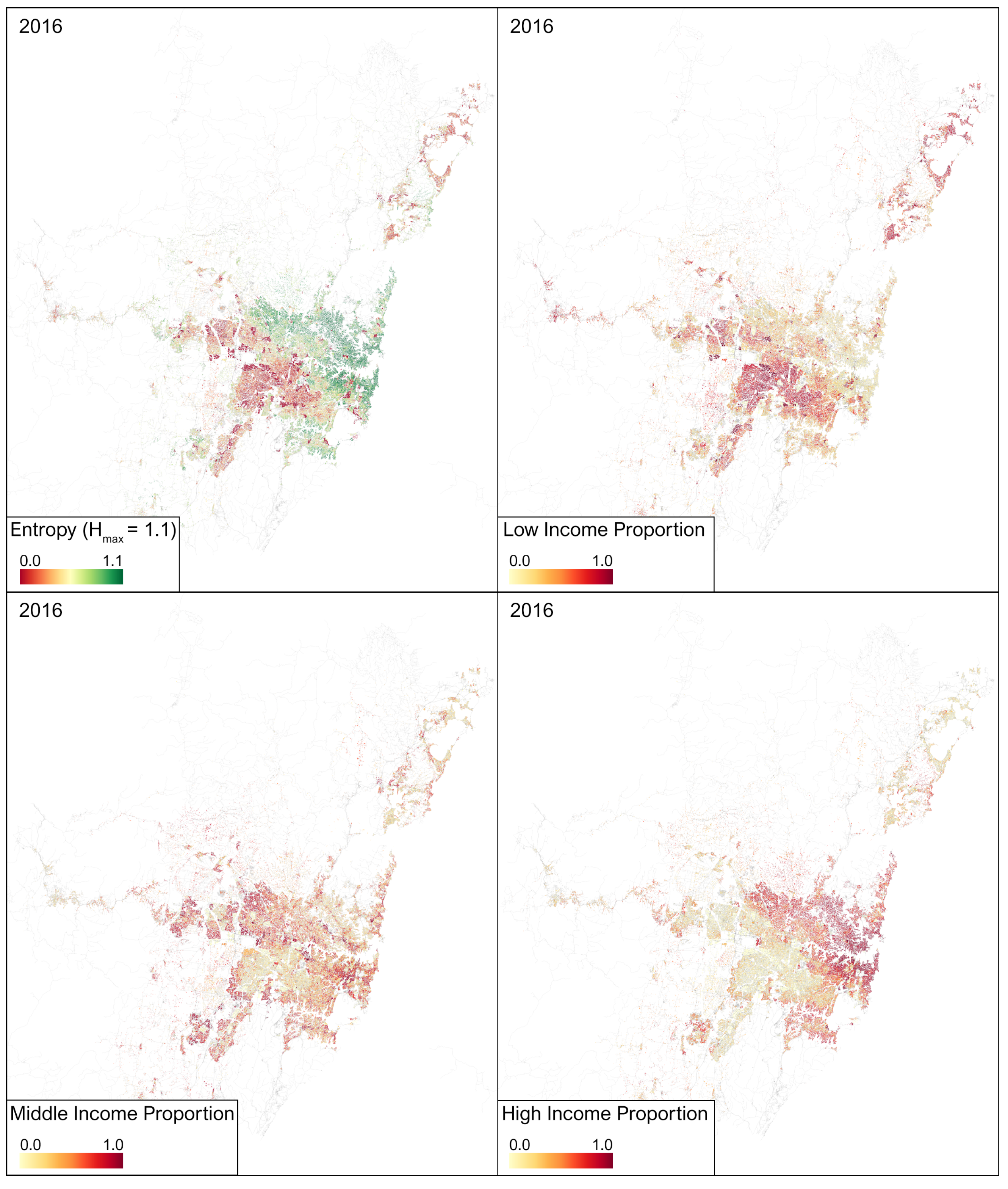
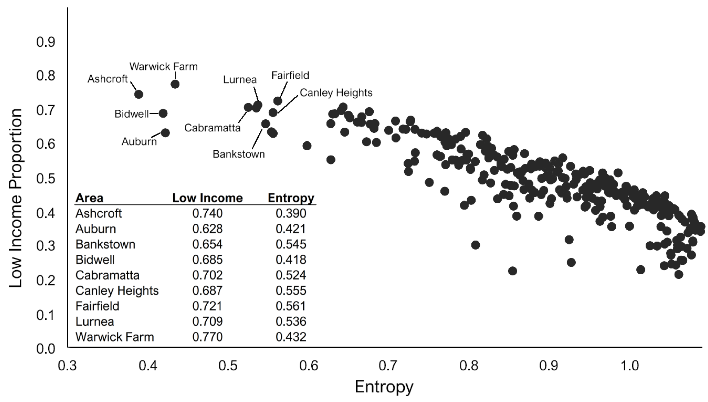
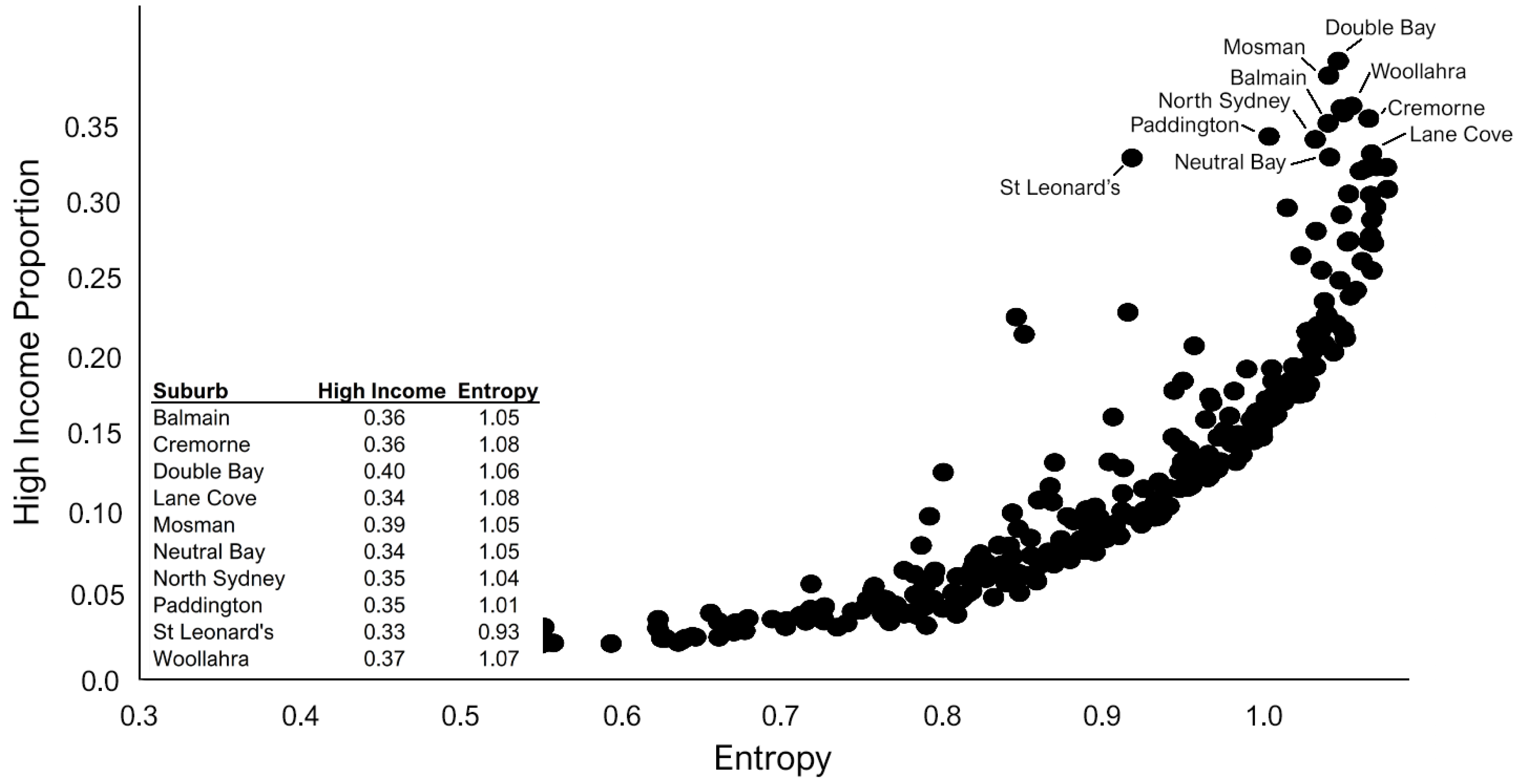
6. Results Objective 1: Income Distributions in Greater Sydney
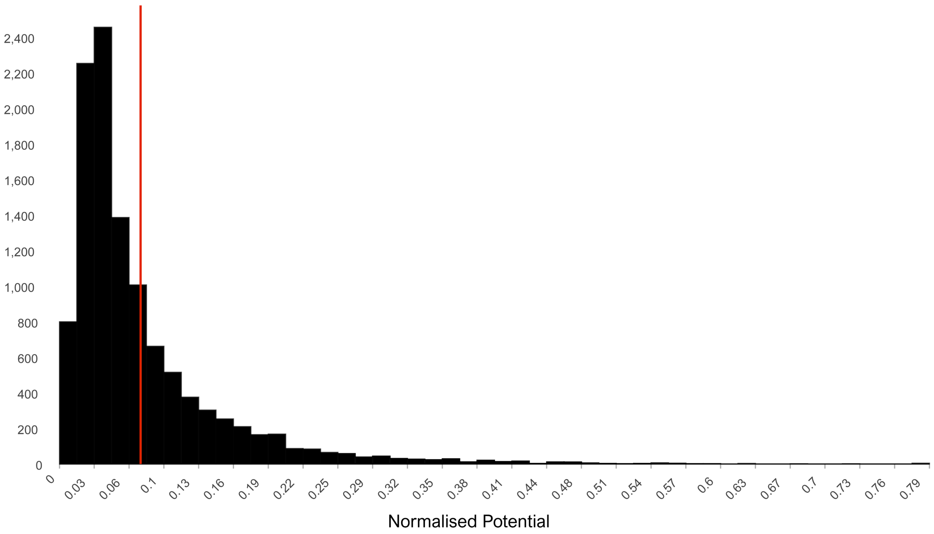
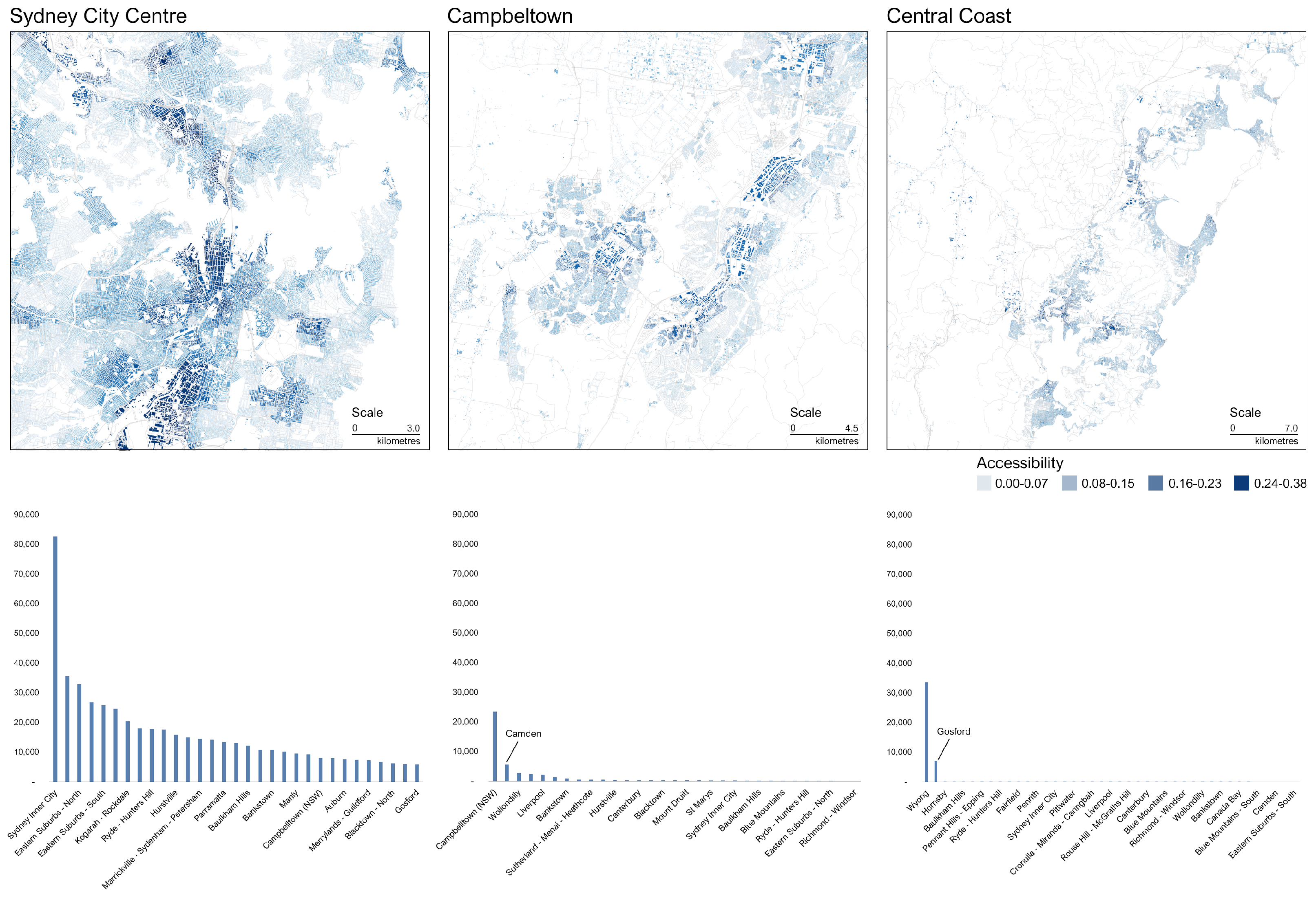
7. Results Objective 2: Accessibility and Income
8. Results Objective 3: House Values, Accessibility, and Income Segregation in Sydney
8.1. Method
8.2. OLS Results
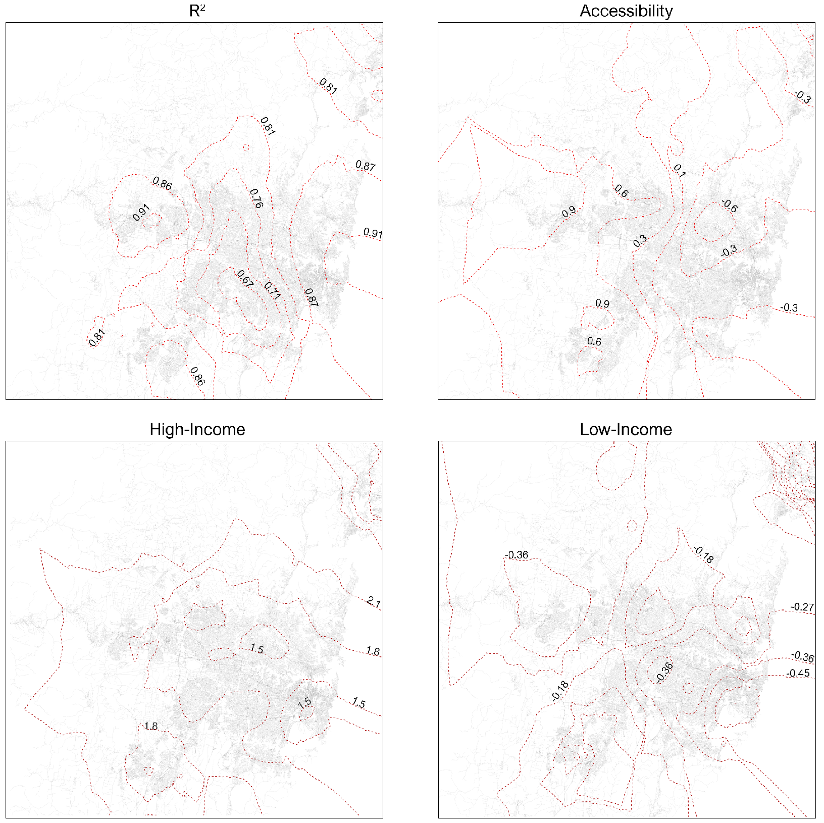
8.3. GWR Results
9. Conclusions
Author Contributions
Funding
Institutional Review Board Statement
Informed Consent Statement
Data Availability Statement
Conflicts of Interest
References
- Kain, J.F. The spatial mismatch hypothesis: Three decades later. Hous. Policy Debate 1992, 3, 371–460. [Google Scholar] [CrossRef]
- Nelson, A.C.; Moore, T. Assessing urban growth management: The case of Portland, Oregon, the USA’s largest urban growth boundary. Land Use Policy 1993, 10, 293–302. [Google Scholar] [CrossRef]
- Ihlanfeldt, K. The spatial mismatch between jobs and residential locations within urban areas. Cityscape 1994, 1, 219–244. [Google Scholar]
- Gobillon, L.; Selod, H.; Zenou, Y. The mechanisms of spatial mismatch. Urban Stud. 2007, 44, 2401–2427. [Google Scholar] [CrossRef] [Green Version]
- Hillier, A.E. Spatial analysis of historical redlining: A methodological exploration. J. Hous. Res. 2003, 14, 137–167. [Google Scholar]
- Dujardin, C.; Goffette-Nagot, F. Neighborhood Effects, Public Housing and Unemployment in France. SSRN Electron. J. 2005. [Google Scholar] [CrossRef] [Green Version]
- Åslund, O.; Östh, J.; Zenou, Y. How important is access to jobs? Old question—Improved answer. J. Econ. Geogr. 2010, 10, 389–422. [Google Scholar] [CrossRef] [Green Version]
- Cervero, R.; Rood, T.; Appleyard, B. Job Accessibility as a Performance Indicator: An Analysis of Trends and Their Social Policy Implications in the San Francisco Bay Area; University of California at Berkeley: Berkeley, CA, USA, 1995. [Google Scholar]
- Mulley, C. Accessibility and residential land value uplift: Identifying spatial variations in the accessibility impacts of a bus transitway. Urban Stud. 2014, 51, 1707–1724. [Google Scholar] [CrossRef]
- Pettit, C.; Shi, Y.; Han, H.; Rittenbruch, M.; Foth, M.; Lieske, S.; Van De Nouwelant, R.; Mitchell, P.; Leao, S.; Christensen, B.; et al. A new toolkit for land value analysis and scenario planning. Environ. Plan. B Urban Anal. City Sci. 2020, 47, 1490–1507. [Google Scholar] [CrossRef]
- Bangura, M.; Lee, C.L. The differential geography of housing affordability in Sydney: A disaggregated approach. Aust. Geogr. 2019, 50, 295–313. [Google Scholar] [CrossRef]
- Randolph, B.; Tice, A. Suburbanizing disadvantage in Australian cities: Sociospatial change in an era of neoliberalism. J. Urban Aff. 2014, 36, 384–399. [Google Scholar] [CrossRef]
- Miller, E.J. Accessibility: Measurement and Application in Transportation Planning. Transp. Rev. 2018, 38, 551–555. [Google Scholar] [CrossRef]
- Páez, A.; Scott, D.M.; Morency, C. Measuring accessibility: Positive and normative implementations of various accessibility indicators. J. Transp. Geogr. 2012, 25, 141–153. [Google Scholar] [CrossRef]
- Masucci, A.P.; Serras, J.; Johansson, A.; Batty, M. Gravity versus radiation models: On the importance of scale and heterogeneity in commuting flows. Phys. Rev. E 2013, 88, 022812. [Google Scholar] [CrossRef] [Green Version]
- Piovani, D.; Arcaute, E.; Uchoa, G.; Wilson, A.; Batty, M. Measuring accessibility using gravity and radiation models. R. Soc. Open Sci. 2018, 5, 171668. [Google Scholar] [CrossRef] [Green Version]
- Yang, R.; Liu, Y.; Liu, Y.; Liu, H.; Gan, W. Comprehensive Public Transport Service Accessibility Index—A New Approach Based on Degree Centrality and Gravity Model. Sustainability 2019, 11, 5634. [Google Scholar] [CrossRef] [Green Version]
- Muraco, W.A. Intraurban Accessibility. Econ. Geogr. 1972, 48, 388–405. [Google Scholar] [CrossRef]
- Vickerman, R.W. Accessibility, attraction, and potential: A review of some concepts and their use in determining mobility. Environ. Plan. A 1974, 6, 675–691. [Google Scholar] [CrossRef] [Green Version]
- Van Eck, J.R.; de Jong, T. Accessibility analysis and spatial competition effects in the context of GIS-supported service location planning. Comput. Environ. Urban Syst. 1999, 23, 75–89. [Google Scholar] [CrossRef]
- Tsou, K.W.; Hung, Y.T.; Chang, Y.L. An accessibility-based integrated measure of relative spatial equity in urban public facilities. Cities 2005, 22, 424–435. [Google Scholar] [CrossRef]
- Sá, C.; Florax, R.J.; Rietveld, P. Does accessibility to higher education matter? Choice behaviour of high school graduates in the Netherlands. Spat. Econ. Anal. 2006, 1, 155–174. [Google Scholar] [CrossRef]
- Cheng, J.; Bertolini, L. Measuring urban job accessibility with distance decay, competition and diversity. J. Transp. Geogr. 2013, 30, 100–109. [Google Scholar] [CrossRef] [Green Version]
- Brondeel, R.; Weill, A.; Thomas, F.; Chaix, B. Use of healthcare services in the residence and workplace neighbourhood: The effect of spatial accessibility to healthcare services. Health Place 2014, 30, 127–133. [Google Scholar] [CrossRef] [PubMed]
- Curl, A.; Nelson, J.D.; Anable, J. Does accessibility planning address what matters? A review of current practice and practitioner perspectives. Res. Transp. Bus. Manag. 2011, 2, 3–11. [Google Scholar] [CrossRef] [Green Version]
- Massey, D.S.; Denton, N.A. The dimensions of residential segregation. Soc. Forces 1988, 67, 281–315. [Google Scholar] [CrossRef]
- Arapoglou, V.P.; Sayas, J. New facets of urban segregation in southern Europe: Gender, migration and social class change in Athens. Eur. Urban Reg. Stud. 2009, 16, 345–362. [Google Scholar] [CrossRef]
- Li, H.; Campbell, H.; Fernandez, S. Residential segregation, spatial mismatch and economic growth across US metropolitan areas. Urban Stud. 2013, 50, 2642–2660. [Google Scholar] [CrossRef]
- Cervero, R. Paradigm shift: From automobility to accessibility planning. Urban Futur. 1997, 22, 9–20. [Google Scholar]
- Geurs, K.T.; Krizek, K.J.; Reggiani, A. Accessibility Analysis and Transport Planning: Challenges for Europe and North America; Edward Elgar Publishing: Cheltenham, UK, 2012. [Google Scholar]
- Bartholomew, K.; Ewing, R. Hedonic price effects of pedestrian-and transit-oriented development. J. Plan. Lit. 2011, 26, 18–34. [Google Scholar] [CrossRef]
- Proffitt, D.G.; Bartholomew, K.; Ewing, R.; Miller, H.J. Accessibility planning in American metropolitan areas: Are we there yet? Urban Stud. 2019, 56, 167–192. [Google Scholar] [CrossRef]
- Lieske, S.N.; van den Nouwelant, R.; Han, J.H.; Pettit, C. A novel hedonic price modelling approach for estimating the impact of transportation infrastructure on property prices. Urban Stud. 2021, 58, 182–202. [Google Scholar] [CrossRef]
- Cutler, D.M.; Glaeser, E.L. Are ghettos good or bad? Q. J. Econ. 1997, 112, 827–872. [Google Scholar] [CrossRef]
- Turner, M.A.; Popkin, S.J.; Rawlings, L. Public Housing and the Legacy of Segregation; The Urban Institute: Washington, DC, USA, 2009. [Google Scholar]
- Fan, Y. The planners’ war against spatial mismatch: Lessons learned and ways forward. J. Plan. Lit. 2012, 27, 153–169. [Google Scholar] [CrossRef]
- Kneebone, E.; Holmes, N. The growing distance between people and jobs in metropolitan America. In Metropolitan Policy Program at Brookings; The Brookings Institution: Washington, DC, USA, 2015. [Google Scholar]
- Geurs, K.T.; Van Wee, B. Accessibility evaluation of land-use and transport strategies: Review and research directions. J. Transp. Geogr. 2004, 12, 127–140. [Google Scholar] [CrossRef]
- Ferrer, A.L.C.; Thomé, A.M.T.; Scavarda, A.J. Sustainable urban infrastructure: A review. Resour. Conserv. Recycl. 2018, 128, 360–372. [Google Scholar] [CrossRef]
- Banister, D. Unsustainable Transport: City Transport in the New Century; Routledge: London, UK, 2005. [Google Scholar]
- Farrington, J.H. The new narrative of accessibility: Its potential contribution to discourses in (transport) geography. J. Transp. Geogr. 2007, 15, 319–330. [Google Scholar] [CrossRef]
- Davidson, K.B. Accessibility and isolation in transport network evaluation. In Proceedings of the VII World Conference on Transport Research, Sydney, Australia, 16–21 July 1995; pp. 8–10. [Google Scholar]
- Ewing, R.H.; Pendall, R.; Chen, D.D. Measuring Sprawl and Its Impact; Smart Growth America: Washington, DC, USA, 2002; Volume 1. [Google Scholar]
- Ewing, R.; Hamidi, S.; Grace, J.B.; Wei, Y.D. Does urban sprawl hold down upward mobility? Landsc. Urban Plan. 2016, 148, 80–88. [Google Scholar] [CrossRef] [Green Version]
- Alesina, A.; Baqir, R.; Easterly, W. Public goods and ethnic divisions. Q. J. Econ. 1999, 114, 1243–1284. [Google Scholar] [CrossRef] [Green Version]
- Alesina, A.; La Ferrara, E. Participation in heterogeneous communities. Q. J. Econ. 2000, 115, 847–904. [Google Scholar] [CrossRef] [Green Version]
- Charles, C.Z. The dynamics of racial residential segregation. Annu. Rev. Sociol. 2003, 29, 167–207. [Google Scholar] [CrossRef] [Green Version]
- Sánchez, F.J.; Liu, W.M.; Leathers, L.; Goins, J.; Vilain, E. The subjective experience of social class and upward mobility among African American men in graduate school. Psychol. Men Masculinity 2011, 12, 368. [Google Scholar] [CrossRef] [PubMed] [Green Version]
- Wasmer, E.; Zenou, Y. Does city structure affect job search and welfare? J. Urban Econ. 2002, 51, 515–541. [Google Scholar] [CrossRef]
- Stoll, M.A. Spatial job search, spatial mismatch, and the employment and wages of racial and ethnic groups in Los Angeles. J. Urban Econ. 1999, 46, 129–155. [Google Scholar] [CrossRef]
- Giuliano, G.; Small, K.A. Is the journey to work explained by urban structure? Urban Stud. 1993, 30, 1485–1500. [Google Scholar] [CrossRef] [Green Version]
- De Bruyne, K.; Van Hove, J. Explaining the spatial variation in housing prices: An economic geography approach. Appl. Econ. 2013, 45, 1673–1689. [Google Scholar] [CrossRef]
- Määttänen, N.; Terviö, M. Income distribution and housing prices: An assignment model approach. J. Econ. Theory 2014, 151, 381–410. [Google Scholar] [CrossRef] [Green Version]
- Ohnishi, T.; Mizuno, T.; Shimizu, C.; Watanabe, T. On the Evolution of the House Price Distribution; Working Paper 249; Center on Japanese Economy and Business, Graduate School of Business, Columbia University: New York, NY, USA, 2011. [Google Scholar]
- Davidson, P.; Saunders, P.; Phillips, J. Inequality in Australia 2018; ACOSS and UNSW Sydney: Strawberry Hills, NSW, Australia, 2018. [Google Scholar]
- AGPC. Rising Inequality? A Stocktake of the Evidence; Australia Government Productivity Commission Research Commission Research Paper; AGPC: Canberra, ACT, Australia, 2018; pp. 1–162. [Google Scholar]
- Sila, U.; Dugain, V. Income, Wealth and Earnings Inequality in Australia: Evidence from the HILDA Survey; OECD Economics Department Working Papers, Working Paper 1538; OECD: Paris, France, 2019. [Google Scholar]
- Wiesel, I.; Ralston, L.; Stone, W. How the Housing Boom Has Driven Rising Inequality. The Conversation 2020. Available online: https://theconversation.com/how-the-housing-boom-has-driven-rising-inequality-102581 (accessed on 18 March 2021).
- Gittins, R. Inequality: Nothing to See Here is Not the True Picture. The Sydney Morning Herald. 2018. Available online: https://www.smh.com.au/business/the-economy/inequality-nothing-to-see-here-is-not-the-true-picture-20180831-p500ww.html (accessed on 17 March 2021).
- ABS. Total PERSONAL Income (Weekly) (INCP); Australian Bureau of Statistics: Sydney, NSW, Australia, 2017.
- ACOSS. Poverty in Australia 2016; The Australian Council of Social Service: Strawberry Hills, NSW, Australia, 2016; pp. 1–41. [Google Scholar]
- PCA. Treasury Laws Amendment (Medicare Levy and Medicare Levy Surcharge) Bill 2019; The Parliament of the Commonwealth of Australia: Canberra, ACT, Australia, 2019; pp. 1–17. Available online: https://www.overleaf.com/project/62d81a25300c236f626b4e9d (accessed on 17 March 2021).
- ABS. Census of Population and Housing Destination Zones; Australian Bureau of Statistics: Canberra, ACT, Australia, 2016. Available online: https://www.abs.gov.au/statistics/people/population/census-population-and-housing-destination-zones/latest-release (accessed on 17 March 2021).
- OpenStreetMap Data in Layered GIS Format Topf J 2009. GeoFabrik, 2009. Available online: https://www.geofabrik.de/data/geofabrik-osm-gis-standard-0.7.pdf (accessed on 17 March 2021).
- Batty, M.; Morphet, R.; Masucci, P.; Stanilov, K. Entropy, complexity, and spatial information. J. Geogr. Syst. 2014, 16, 363–385. [Google Scholar] [CrossRef] [Green Version]
- Wilson, A. Entropy in Urban and Regional Modelling (Routledge Revivals); Routledge: London, UK, 2013. [Google Scholar]
- Tan, Y.; Wu, C.F. The laws of the information entropy values of land use composition. J. Nat. Resour. 2003, 18, 112–117. [Google Scholar]
- Fischer, M.J. The relative importance of income and race in determining residential outcomes in US urban areas, 1970–2000. Urban Aff. Rev. 2003, 38, 669–696. [Google Scholar] [CrossRef]
- Hansen, W.G. How accessibility shapes land use. J. Am. Inst. Planners 1959, 25, 73–76. [Google Scholar] [CrossRef]
- Luo, J. Integrating the Huff model and floating catchment area methods to analyze spatial access to healthcare services. Trans. GIS 2014, 18, 436–448. [Google Scholar] [CrossRef]
- Kantorovich, Y.G. Equilibrium models of spatial interaction with locational-capacity constraints. Environ. Plan. A 1992, 24, 1077–1095. [Google Scholar] [CrossRef]
- Hernández-Murillo, R.; Owyang, M.T. The information content of regional employment data for forecasting aggregate conditions. Econ. Lett. 2006, 90, 335–339. [Google Scholar] [CrossRef] [Green Version]
- Geurs, K.T.; De Montis, A.; Reggiani, A. Recent advances and applications in accessibility modelling. Comput. Environ. Urban Syst. 2015, 49, 82–85. [Google Scholar] [CrossRef] [Green Version]
- Dennett, A. Estimating Flows between Geographical Locations: ‘Get Me Started in’ Spatial Interaction Modelling; Technical Report; UCL: London, UK, 2012. [Google Scholar]
- Wilson, A.G. A family of spatial interaction models, and associated developments. Environ. Plan. A 1971, 3, 1–32. [Google Scholar] [CrossRef] [Green Version]
- Fotheringham, A.S.; Brunsdon, C.; Charlton, M. Geographically Weighted Regression: The Analysis of Spatially Varying Relationships; John Wiley & Sons: Hoboken, NJ, USA, 2003. [Google Scholar]
- Fotheringham, A.S.; Oshan, T.M. Geographically weighted regression and multicollinearity: Dispelling the myth. J. Geogr. Syst. 2016, 18, 303–329. [Google Scholar] [CrossRef]
- Oshan, T.; Wolf, L.J.; Fotheringham, A.S.; Kang, W.; Li, Z.; Yu, H. A comment on geographically weighted regression with parameter-specific distance metrics. Int. J. Geogr. Inf. Sci. 2019, 33, 1289–1299. [Google Scholar] [CrossRef]
- Albuquerque, P.H.M.; Medina, F.A.S.; Silva, A.R.D. Geographically weighted logistic regression applied to credit scoring models. Rev. Contab. Financ. 2017, 28, 93–112. [Google Scholar] [CrossRef] [Green Version]
- Fábián, Z. Method of the Geographically Weighted Regression and an Example for its Application. Reg. Stat. 2014, 1, 61–75. [Google Scholar] [CrossRef]
- Gareth, J.; Daniela, W.; Trevor, H.; Robert, T. An Introduction to Statistical Learning: With Applications in R; Springer: New York, NY, USA, 2013. [Google Scholar]
- Bruce, P.; Bruce, A.; Gedeck, P. Practical Statistics for Data Scientists: 50+ Essential Concepts Using R and Python; O’Reilly Media: Sebastopol, CA, USA, 2020. [Google Scholar]
- Lee, C.L.; Piracha, A.; Fan, Y. Another Tale of Two Cities: Access to Jobs Divides Sydney Along the ‘Latte Line’. The Conversation 2018. Available online: https://theconversation.com/another-tale-of-two-cities-access-to-jobs-divides-sydney-along-the-latte-line-96907 (accessed on 17 March 2021).
- Australian Bureau of Statistics. Media Release—More than Two in Three Drive to Work, Census Reveals (Media Release), Australian Bureau of Statistics, Release 133/2017. 2017. Available online: https://www.abs.gov.au/ausstats/abs@.nsf/mediareleasesbyreleasedate/7DD5DC715B608612CA2581BF001F8404?OpenDocument (accessed on 17 March 2021).


| Dataset | Source |
|---|---|
| Road Network | OpenStreetMap |
| Statistical Area 2 Neighbourhood Attributes | Australian Bureau of Statistics |
| Journey to Work | Australian Bureau of Statistics |
| Income Data | Australian Bureau of Statistics |
| Geographic Statistical Boundaries | Australian Bureau of Statistics |
| House Price | Australian Property Monitor |
| Points of Interest (including building footprints) | Geoscape Australia |
| Classification | Line Count | Total Length (km) |
|---|---|---|
| Motorway | 11,220 | 2466 |
| Primary | 10,305 | 1755 |
| Residential | 178,668 | 23,203 |
| Secondary | 16,705 | 2537 |
| Shared | 116 | 12 |
| Tertiary | 23,495 | 3141 |
| Tracks | 10,286 | 6530 |
| Unclassed | 8716 | 2363 |
| Total | 259,511 | 42,007 |
| Low Income | Middle Income | High Income | Entropy | |
|---|---|---|---|---|
| Low Income | 1.000 | −0.218 | −0.561 | −0.219 |
| Middle Income | −0.218 | 1.000 | 0.198 | 0.565 |
| High Income | −0.561 | 0.198 | 1.000 | 0.629 |
| Entropy | −0.219 | 0.565 | 0.629 | 1.000 |
| Residuals: | |||||
|---|---|---|---|---|---|
| Min | 1Q | Median | 3Q | Max | |
| −3.08558 | −0.14556 | −0.01844 | 0.11633 | 2.40827 | |
| Coefficients: | |||||
| Estimate | Std. Error | t-Value | Pr (>|t|) | ||
| (Intercept) | 1.33 × 10 | 5.69 × 10 | 233.182 | <2.00 × 10 | *** |
| Bedrooms | 1.42 × 10 | 1.58 × 10 | 90.152 | <2.00 × 10 | *** |
| Bathrooms | 4.89 × 10 | 1.48 × 10 | 33.016 | <2.00 × 10 | *** |
| Distance to Sydney | −1.45 × 10 | 1.69 × 10 | −85.66 | <2.00 × 10 | *** |
| Distance to Secondary City | 7.07 × 10 | 1.74 × 10 | 4.065 | 4.82 × 10 | *** |
| Distance to Beach | −2.44 × 10 | 2.24 × 10 | −10.916 | <2.00 × 10 | *** |
| Distance to Bus Interchanges | 2.91 × 10 | 4.83 × 10 | 6.031 | 1.65 × 10 | *** |
| Distance to Highway | 7.50 × 10 | 4.44 × 10 | 16.883 | <2.00 × 10 | *** |
| Distance to Primary School | 1.02 × 10 | 3.26 × 10 | 3.118 | 0.00182 | ** |
| Distance to University | 1.12 × 10 | 4.27 × 10 | 2.617 | 0.00889 | ** |
| Distance to Swimming Pool | −4.61 × 10 | 9.32 × 10 | −4.952 | 7.40 × 10 | *** |
| Distance to Shopping Centre | 1.11 × 10 | 7.50 × 10 | 14.774 | <2.00 × 10 | *** |
| Distance to Sport Centre | 9.00 × 10 | 7.27 × 10 | 12.378 | <2.00 × 10 | *** |
| Population Above 65 (%) | 5.08 × 10 | 2.17 × 10 | 23.355 | <2.00 × 10 | *** |
| Crime Rate (%) | −4.35 × 10 | 1.62 × 10 | −2.681 | 0.00735 | ** |
| Low Income (%) | −1.87 × 10 | 5.75 × 10 | −3.244 | 0.00118 | ** |
| Middle Income (%) | −1.02 × 10 | 5.80 × 10 | −1.758 | 0.0788 | . |
| High Income (%) | 2.51 | 5.97 × 10 | 41.983 | <2.00 × 10 | *** |
| Accessibility Score | 2.73 × 10 | 8.68 × 10 | 3.142 | 0.00168 | ** |
| Summary of GWR Coefficient Estimates | |||||
|---|---|---|---|---|---|
| Min | 1Q | Median | 3Q | Max | |
| Intercept | 6.2 | 1.3 × 10 | 1.4 × 10 | 1.4 × 10 | 1.8 × 10 |
| Bedrooms | 1.1 × 10 | 1.2 × 10 | 1.4 × 10 | 1.6 × 10 | 1.9 × 10 |
| Bathrooms | 2.8 × 10 | 4.0 × 10 | 5.1 × 10 | 5.8 × 10 | 8.1 × 10 |
| Distance to Sydney | −3.4 × 10 | −3.0 × 10 | −2.3 × 10 | −1.5 × 10 | 0.0 |
| Distance to Secondary City | −1.6 × 10 | −4.7 × 10 | −5.6 × 10 | 4.1 × 10 | 0.0 |
| Distance to Beach | −3.8 × 10 | −8.7 × 10 | 2.3 × 10 | 8.7 × 10 | 0.0 |
| Distance to Bus Interchanges | −3.8 × 10 | −9.7 × 10 | −3.2 × 10 | 4.4 × 10 | 0.0 |
| Distance to Highway | −1.8 × 10 | 3.0 × 10 | 7.6 × 10 | 1.1 × 10 | 0.0 |
| Distance to Primary School | −3.7 × 10 | 1.3 × 10 | 2.7 × 10 | 4.5 × 10 | 1.0 × 10 |
| Distance to University | −2.1 × 10 | 2.3 × 10 | 6.5 × 10 | 1.1 × 10 | 0.0 |
| Distance to Swimming Pool | −2.7 × 10 | −1.3 × 10 | -4.5 × 10 | 6.8 × 10 | 0.0 |
| Distance to Shopping Centres | −1.5 × 10 | −4.0 × 10 | 7.2 × 10 | 1.8 × 10 | 0.0 |
| Distance to Sports Centres | −1.2 × 10 | 3.6 × 10 | 6.7 × 10 | 1.4 × 10 | 0.0 |
| Population Above 65 | 1.2 × 10 | 2.6 × 10 | 3.7 × 10 | 5.8 × 10 | 8.9 × 10 |
| Crime Rate | −3.1 × 10 | −8.0 × 10 | −2.1 × 10 | 1.0 × 10 | 6.8 × 10 |
| Low Income (%) | −7.2 | −3.8 × 10 | −2.8 × 10 | −1.6 × 10 | 5.0 |
| Middle Income (%) | −6.6 | −3.1 × 10 | −1.8 × 10 | −6.7 × 10 | 5.4 |
| High Income (%) | −4.5 | 1.5 | 1.7 | 1.8 | 7.7 |
| Accessibility Score | −7.8 × 10 | −2.8 × 10 | 3.3 × 10 | 5.7 × 10 | 1.1 |
Publisher’s Note: MDPI stays neutral with regard to jurisdictional claims in published maps and institutional affiliations. |
© 2022 by the authors. Licensee MDPI, Basel, Switzerland. This article is an open access article distributed under the terms and conditions of the Creative Commons Attribution (CC BY) license (https://creativecommons.org/licenses/by/4.0/).
Share and Cite
Ng, M.K.M.; Roper, J.; Lee, C.L.; Pettit, C. The Reflection of Income Segregation and Accessibility Cleavages in Sydney’s House Prices. ISPRS Int. J. Geo-Inf. 2022, 11, 413. https://doi.org/10.3390/ijgi11070413
Ng MKM, Roper J, Lee CL, Pettit C. The Reflection of Income Segregation and Accessibility Cleavages in Sydney’s House Prices. ISPRS International Journal of Geo-Information. 2022; 11(7):413. https://doi.org/10.3390/ijgi11070413
Chicago/Turabian StyleNg, Matthew Kok Ming, Josephine Roper, Chyi Lin Lee, and Christopher Pettit. 2022. "The Reflection of Income Segregation and Accessibility Cleavages in Sydney’s House Prices" ISPRS International Journal of Geo-Information 11, no. 7: 413. https://doi.org/10.3390/ijgi11070413
APA StyleNg, M. K. M., Roper, J., Lee, C. L., & Pettit, C. (2022). The Reflection of Income Segregation and Accessibility Cleavages in Sydney’s House Prices. ISPRS International Journal of Geo-Information, 11(7), 413. https://doi.org/10.3390/ijgi11070413