Geo-Referencing and Analysis of Entities Extracted from Old Drawings and Photos Using Computer Vision and Deep Learning Algorithms

Abstract

This study offers a quantitative solution that automates the creation of a historical timeline starting with old drawings from the beginning of the 18th century and ending with present-day photographs of the Old City of Jerusalem. This is performed using GIScience approaches, computer vision, and deep learning. The motivation to select the Old City of Jerusalem is the substantial availability of old archival drawings and photographs, owing to the area’s significance throughout the years. This task is challenging, as drawings, old photographs, and new photographs exhibit distinct characteristics. Our method encompasses several key components for the analyses: a 2D location recommendation engine, which detects an approximate location in the image of 3D landmarks; 2D landmarks to 3D conversion; and 2D polygonal areas to 3D GIS polylines conversion. This is applied to the segmentation of built areas. To achieve more accurate results, Meta’s Segment Anything model was utilized, which eliminates the need for extensive data preparation, training, and validation, thus optimizing the process. Using such techniques enabled us to examine the landscape development throughout the last three centuries and gain deeper insights concerning the evolution of prominent landmarks and features such as built area over time.

1. Introduction

Accurate visual sources play a critical role in the reconstruction of historical landscapes. Among them, old photographs are one of the most valuable and precise sources available [1,2]. However, because photography was not available prior to the mid-19th century [3], researchers must rely on alternative visual sources and cartographic material. However, while these sources provide valuable information, they can be incomplete, inaccurate, and subjective, necessitating careful verification [4,5]. Additionally, many of these sources lack geo-referencing to a modern coordinate reference system (CRS), making it challenging to accurately position the depicted features within a spatial context. The process of verifying visual historical sources is complex, time-consuming, and often requires specialized professional skills [4]. Moreover, visual sources encompass a variety of types, including maps, photographs, drawings, and sketches, each exhibiting unique spatial settings, characteristics, origins, styles, and production standards. Integrating and cross-correlating these diverse sources can present challenges in terms of achieving uniformity, compatibility, and suitability for analysis [6,7,8,9].

Our case study is on landmarks and building areas in the Old City of Jerusalem, where the availability of old photographs is limited to the mid-19th century onward. As a result, our reliance on old drawings depicted prior to this period becomes essential for landscape reconstruction. The primary motivation for our selection of the Old City of Jerusalem is the substantial availability of old archival drawings and photographs, owing to the area’s enduring significance throughout the years. Many studies have examined Jerusalem using such sources. For example, the inspection of drawings and painters in conjunction with historical events [10], the examination of Jerusalem’s maps [11], photography as a major tool for depicting Jerusalem in the 19th century [12]. Yet, most of the existing studies conducted so far are qualitative, thus ignoring the vast potential of performing quantitative analyses to gain more accurate and enriched insights.

In this paper, we developed a unified framework designed to analyze a set of drawings and photos, each with its unique characteristics and behaviors. Using this framework, one can determine the precise location from where a drawing or photo was taken and establish a connection between the 2D pixels of the drawing/photo and their corresponding 3D real-world GIS points. This connection enables us to seamlessly convert 3D GIS points to the 2D pixels of the drawing/photo and vice versa. With this capability, we can perform geo-referencing on a given drawing, allowing us to accurately position it within the spatial context. Furthermore, one can effortlessly switch between the 2D representation of the drawing/photo and its corresponding 3D point in the real world, opening up new possibilities for comprehensive analysis and interpretation of historical and geographical data.

Performing such tasks tackles the persistent challenge of accuracy in the domain of drawings by presenting innovative and effective tools. Through the design of these algorithms, we achieve efficient extraction of relevant information from a large number of drawings and photos, enabling us to analyze and interpret depicted scenes with greater precision. One significant aspect is the ability to track changes in landmarks over time, allowing to identify peculiar landmarks within the depicted scenes. This analysis provides valuable insights into the historical development and transformation of the Old City, shedding light on its evolution through the ages. Additionally, our framework tracks landmarks within the drawings and photos that might not be immediately recognizable qualitatively. This feature is invaluable in identifying and interpreting elements that have undergone changes but lack sufficient documentation. By pinpointing these subtle variations, we gain a deeper understanding of the historical context and the reasons behind specific alterations in the Old City. Moreover, our framework can closely examine how particular areas, especially built areas, have evolved over time. This quantitative analysis is unique and may reveal unique patterns or areas of interest, providing crucial insights into the historical urban development and architectural changes that have occurred in the Old City. The developed framework offers a consistent evaluation of the reliability and precision of the depicted information, thereby enhancing the credibility and integrity of the historical analysis. By employing the tools and approaches demonstrated in this study, one can contribute to a more accurate and comprehensive understanding of historical landscapes depicted in artworks, enriching our knowledge of the Old City’s heritage and development beyond the existing knowledge.

2. Related Work and Contributions of This Study

Related works in the field of geographical and historical analysis of old drawings have historically relied on qualitative methods, where researchers visually inspect and interpret the cartographic material. One such example is [13], which qualitatively assessed the Al-Nabi Da’ud minaret’s height in old photos and drawings or [2] analyzing old photographs to extract earthquake damage after the 1927 Jericho earthquake. Another example of qualitative methods can be found in [14], where researchers sought to identify the locations where landscapes were painted by combining information about drawings, their authors, and terrain analysis in GIScience. While qualitative analyses have offered valuable insights, they have limitations in objectivity, accuracy, and reliability, and may not fully exploit modern technologies.

In contrast, some studies have adopted manual quantitative analysis from aerial photography, such as [15]. These approaches integrated aerial reconnaissance photography with conventional census methods to accurately count the nomadic Bedouin population’s tents in the Negev region. Aerial photography was also used in [16], examining Mandatory Palestine during World War I. Recent advancements in deep learning have paved the way for quantitative analyses using sophisticated techniques. The work presented in [17] demonstrates how satellite imagery can be leveraged to build a population map without the need for costly and time-consuming government censuses. The study introduced two convolutional neural network (CNN) architectures to predict population density accurately using inputs from multiple satellite imagery sources. Additionally, Ref. [18] showcases the use of context-based machine learning for extracting human settlement footprints from historical topographic maps. While the detection of areas with no buildings or urban areas achieved good results, individual built area extraction still presents segment detection challenges (individual buildings were not well identified by their model). These diverse works highlight the evolving landscape of geographical and historical analysis, transitioning from qualitative to quantitative approaches and showcasing the potential of deep learning in this domain [19,20]. The integration of innovative techniques continues to open new possibilities for extracting valuable insights from old drawings and maps, contributing to a deeper understanding of historical landscapes.

The work presented in [21] offers a comprehensive exploration of the integration of GIScience within the context of historical geography, specifically focusing on the late Ottoman and Mandatory Palestine. This study examines the potential advantages, obstacles, and complexities associated with incorporating GIScience methodologies into historical geographic analysis. The study emphasizes the significant theoretical and methodological advancements that can be achieved through proper integration, thereby enhancing the field of historical geography and contributing to a deeper understanding of the studied periods.

Our work, which relates images or drawings to a 3D scene (GIS model), is based on research that has been performed in the field of photogrammetry or multiple-view geometry in computer vision. The related issues are covered for example in [22] in chapters 9–13. In brief, given a set of 3D points and their corresponding points in an image, the place where the image was taken O and the homography matrix H (an uncalibrated projection matrix) can be estimated. Using them, a projection of 3D points to the image can be computed, and given a point in the image, the corresponding 3D ray can be computed. We will be using these capabilities as a basis for our algorithms described below.

The most recent work closely related to our study is [23]. This previous work focuses on determining the location from where a drawing or photo was taken and converts 3D real-world GIS points to 2D landmarks of the drawing/photo. Our study follows [23] and presents innovative improvements. Firstly, we tackle the more challenging task of converting 2D landmarks to 3D real-world GIS points, where information on the Z axis is missing. This conversion requires a technique to accurately infer the missing spatial dimension. Additionally, our study introduces the use of a landmark recommendation engine in old drawings, enabling us to track changes in landmarks over time and identify peculiar landmarks within the depicted scenes. Secondly, our research introduces an approach to examine how specific areas, particularly built areas, have evolved over time. This method is of great importance in landscape reconstruction, in particular during periods in which photographs were not available. Lastly, our study enables assessment of the accuracy of the drawings and photos through a 3D quantitative evaluation, enhancing the credibility and integrity of our historical analysis. By grounding our interpretations in empirical evidence and solid data, we aim to make a more reliable and comprehensive understanding of the depicted scenes. These innovations significantly contribute to the domain of historical geography that examines landscape developments as a proxy for human activity [21]. In our case, we enrich our knowledge associated with Jerusalem Old City’s heritage and development throughout history.

3. Materials and Methods

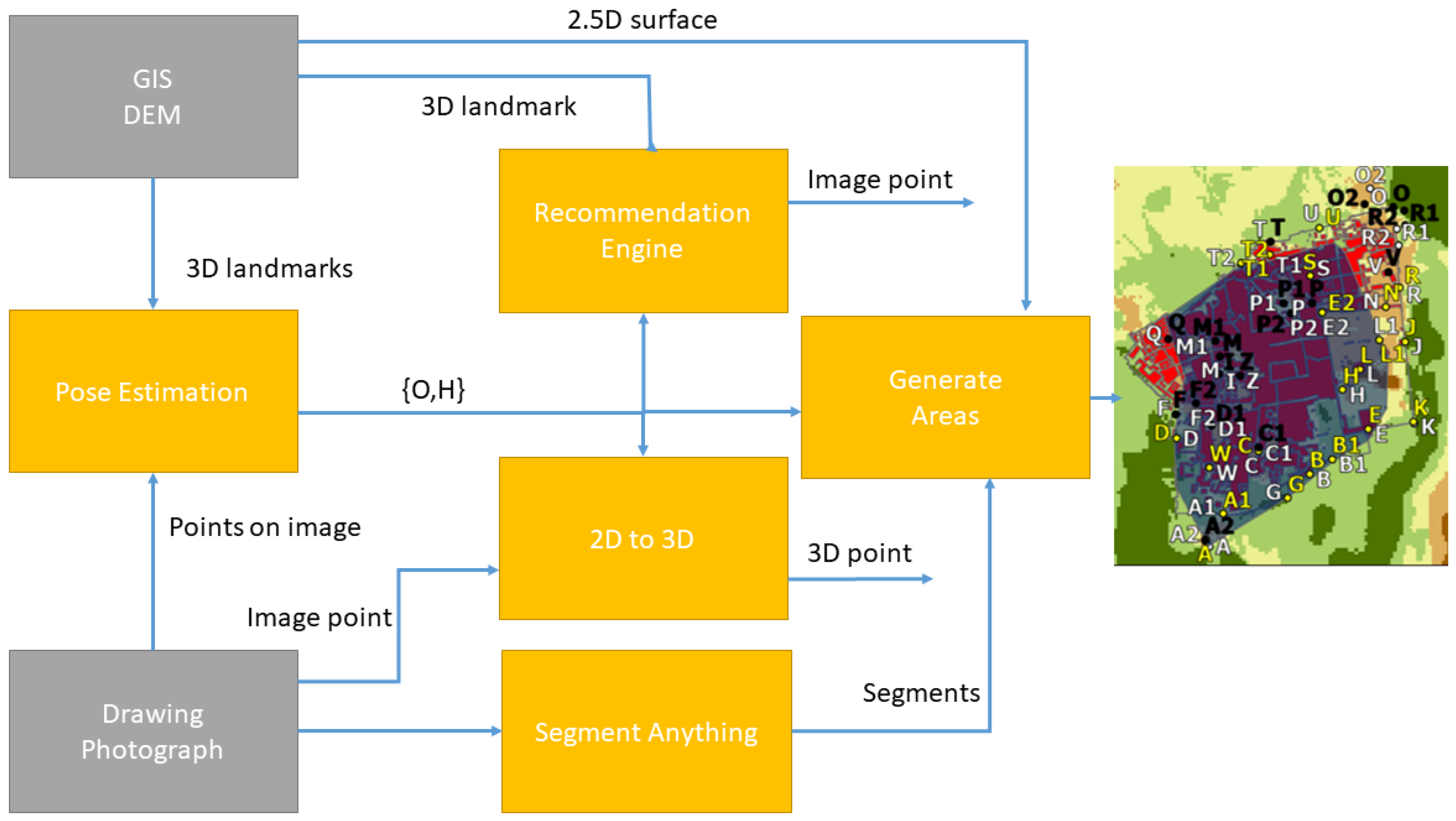
Our methodology comprehensively outlines the algorithms that constitute our unified framework, enabling us to conduct a thorough analysis of old artworks depicting the Old City of Jerusalem. The general outline of the system is given in Figure 1. Using the method described in [23], matches between 3D landmarks and their corresponding points in the image/drawing are used to recover the position of the camera/artist with respect to the 3D scene ($O,H$). This can then be used to find corresponding points between 3D and 2D points. Then, using the DEM (digital elevation model) of the old city, we generate a large 2.5D point cloud (that is, the height represents the surface height in meters above sea level). It is then used to recover the corresponding point in the point cloud for any point in the image.

These capabilities are the basis of our algorithms. Our first algorithm (recommendation engine in the diagram), powered by the location recommendation engine, tracks changes in landmarks over time using 2D drawings and photos. This engine suggests locations within the drawings and photos that may not be immediately recognizable, enhancing our understanding of evolving historical features. The second algorithm (2D to 3D in the diagram) focuses on 3D landmark detection, where we employ computer vision techniques to convert 2D landmarks from drawings and photos into 3D real-world GIS points. Lastly, the third algorithm (generate areas in the diagram) facilitates 3D area generation from drawings and photos. Using deep learning image segmentation techniques, we recover the built areas shown in the picture and convert it to their corresponding detailed 3D areas in the depicted scenes.

The old drawings and photos used to portray the Old City of Jerusalem from the Mount of Olives perspective include De Bruyn’s drawing [24] (1700); Trion’s drawing [25] (1732); Jerusalem [Cartographic Material] drawing [26] (1782); Vue Générale de Jérusalem drawing [27] (1800?); Henniker’s drawing [28] (1823); Vue du Mont des Oliviers, Panorama [29] (1859–1861); Vue du Mont des Oliviers, center, Panorama [30] (1870–1871); Panorama photograph—American Colony [31] (1899–1904); American Colony photograph [32] (1920); American Colony photograph [33] (1934–1939); and Gotfryd, Bernard, photographer [34] (1971). Additionally, there are more recent photos taken by the authors in 2020, namely DSC_0518 photo (2020) and DSC_0539 photo (2020). In addition to old drawings and photographs, we have used present-day orthophotos and DEMs of the Old City of Jerusalem for 2D and 3D locations representation (in terms of coordinates), respectively. The CRS (coordinate reference system) used for extracting the longitude and latitude coordinates is ITM (Israel transverse Mercator) [35], while the elevation values were expressed in absolute height (in meters) above sea level.

3.1. Location Recommendation Engine for 2D Drawings/Photos

Our study presents a location recommendation system tailored specifically for drawings and photographs. The users can mark landmarks they recognize within the image. Our system provides recommendations for landmarks that the user may not have identified initially. This approach not only enhances the user’s exploration of old drawings but also extends to old photos, expanding the range of available resources. The location recommendation system introduces two key innovations. Firstly, it assists users in uncovering unfamiliar landmarks within old drawings/photos. By suggesting additional landmarks that were not initially recognized, users can gain a more comprehensive understanding of the depicted scene and delve into unexplored areas. This contributes to the preservation and interpretation of historical artworks. Secondly, our system enables the observation of landmark evolution over time. Through the analysis of old drawings and photos, users can witness the changes and transformations that landmarks have undergone throughout history. This offers valuable insights into the development and evolution of significant sites and landmarks, providing a unique perspective on the cultural and historical context.

In our study, we include drawings from 1700 (the Renaissance period) and onward, drawn according to established artistic conventions. Thus, these drawings are comparable to photographs. Consequently, we assume that photographic principles apply to drawing, and a model effective for photography also works for drawings. Within the drawings, there are 40 annotated landmarks. However, a potential issue might arise, as some of these landmarks may not align accurately. This discrepancy could stem from errors made by those marking the landmarks, or from the fact that the projection from the 3D landmark to its corresponding 2D landmark in the drawing might be less precise than in photographs. This imprecision could result in outcomes that are less accurate. Therefore, the algorithm should consider that some of the alignments between landmarks in the drawing and real-world coordinates may not be accurate.

One of the crucial technical challenges we addressed in our research involves the estimation of the homography matrix H, which establishes the relationship between a 2D landmark in the drawing and its corresponding 3D real-world coordinate, as well as the camera position O, representing the location from which the drawing or photograph was captured. In a previous work [23], which focused on the Old City of Jerusalem viewed from the Mount of Olives, a method was developed to determine homography matrix and camera position by leveraging 40 known landmarks (depicted in Figure A1 in Appendix A) with their corresponding locations in both the drawing and 3D GIS space. That is, a 2D location on the drawing (in pixels) and the actual surface location in terms of longitude (X ), latitude (Y), and height (Z) coordinates. The longitude and latitude were extracted from the orthophoto, while the height was first extracted from the DEM (the surface height in meters above sea level) and then added to the height of the given structure above the surface. Through this approach, estimates were found for the camera position O and homography matrix H. With these estimates in place, the 2D pixel coordinates $\tilde{p}=(u,v,1)$ can be calculated on the drawing or photo from a given 3D real-world GIS point $P=(X,Y,Z)$. This calculation is achieved through the equation: $H(P-O)\cong \tilde{p}$.

In this current study, we have improved the algorithm to enhance the accuracy and performance of the estimation process. We employed a robust algorithm to align landmarks in the illustration with real-world coordinates. Thus, the algorithm has to estimate the model $(H,O)$ while eliminating outlier matches. Here, we used two versions. The first version employs the RANSAC [36] algorithm, which does not assume that every pair of (landmark, coordinate) matches perfectly. Therefore, a threshold is set, and if the distance exceeds this threshold, the pair is considered inaccurate and it is disregarded. We utilized the RANSAC implementation with a threshold of either 120 or 1000. The second version involves the use of the least-median of squares robust method [37], where decisions are made about which pairs to exclude based on high distance values between them. By incorporating these options into our algorithm, we aim to obtain better and more precise results. These enhancements contribute to the overall accuracy and reliability of our homography matrix estimation, facilitating more robust and accurate transformations between 3D to 2D points. Also, we expanded the scope of our algorithm by testing it on a significantly larger and more diverse dataset of drawings and photos. This expansion allowed us to evaluate the algorithm’s performance and robustness across various artistic styles, time periods, and visual representations of the Old City of Jerusalem.

3.2. Building 2.5D Point Cloud

Our objective is to establish a connection between the 3D real-world geographic information system (GIS) data of the Old City of Jerusalem and the corresponding 2D pixels in the drawings and photographs. To accomplish this, we constructed a geographic 2.5D point cloud that accurately describes the 2.5D surface of the Old City of Jerusalem. To create the point cloud, we first obtained the building layer of the Old City of Jerusalem [38] from 2020 and ensured that only polygonal structures within the Old City will remain. Subsequently, we extracted approximately 100,000 2D points, denoted as R, extending the area of the remaining buildings. Then, we combined the 2D points with the Jerusalem height map [39] to yield a 2.5D point cloud where the elevation of each point (the Z axis) is the height of the surface above sea level (in meters). Obviously, there might be some differences between present-day built area (and consequently also the resulted point cloud) and the past landscape, but we assume that the majority of landmarks have remained stationary for the past 300 years. The resulting geographic 2.5D point cloud serves as a valuable resource for the next analyses and the understanding of the spatial characteristics of the Old City of Jerusalem.

3.3. From 2D Drawing/Photo Landmark to 3D Coordinate

Using the method described in Section 3.1, the camera’s position and the matrix H have been determined. Given a 2D pixel landmark $p=(u,v,1)$ in a drawing/photograph, we aim to determine its corresponding 3D coordinate $P=(X,Y,Z)$. In Section 3.2, we explained how we generated a 2.5D point cloud containing around 100,000 points. Subsequently, we projected this point cloud onto the drawing/photograph. Our framework uses the KDTree algorithm [40] to select points from the point cloud that were 2D projected onto the drawing/photograph, which are the close to the marked landmark. From these points, we select only the 3D points which are closest to the camera as can be seen in Figure 2. From this set of points, the three points whose projections are closet to the marked landmark are selected. Given the density of points, we can assume that these points will nearly always belong to the same building as the marked landmark, and that the vector P is orthogonal to the ray V. Among these chosen points, a single point is selected based on the smallest value of $\left|d\right|$ which measures the distance between P (the real corresponding 3D coordinate) and $\tilde{P}$ (the computed corresponding 3D coordinate), as illustrated in Figure 2. The primary challenge lies in the absence of the Z dimension in a 2D photo/drawing, necessitating its computation.

Given the three Ps, we want to compute the 3D point $\tilde{P}$. To achieve this, we must establish values for V (each 2D pixel p in the drawing/photo corresponds to a 3D ray V), $\alpha$ (the distance from $\tilde{P}$ to the camera position O along the ray V), and d the vector connecting P and $\tilde{P}$), as depicted in Figure 2. Thus, the vector $P-O$ is divided into two orthogonal vectors $\tilde{P}-O$ and d. Using orthogonal vectors yields the shortest vector d. From the three suggested Ps, the one with the shortest vector d will be chosen.

Initially, our focus is on finding V. From the previous study [23], we derived the equation $\tilde{p}\cong H(\tilde{P}-O)$. This previous study transitioned from 3D to 2D and calculated the 2D point $\tilde{p}$, but this current study transitioned from 3D to 2D to obtain the ray V due to the absence of the Z dimension in a 2D photo/drawing. To proceed, both sides of the equation are multiplied $H^{-1}$, resulting in:

$$H^{-1}p\cong (\tilde{P}-O)\cong V.$$

(1)

Next, we established $\alpha$, which is the size of the vector $\tilde{P}-O$. This yields a point on the ray V so $\tilde{P}-O=\alpha V$):

$$P-O=(\tilde{P}-O)+d=\alpha V+d.$$

(2)

For the distance $\alpha$ to be in meters, it is necessary for V to be a unit vector. Therefore, we normalize V, ensuring that $V^{T}V=1$. As d is orthogonal to V ($d\perp V$), we arrive at the relationship $d^{T}V=0$. By multiplying both sides of this equation by $V^T$, we attain the value of $\alpha$.

$$V^T(P-O)=V^T(\alpha V+d)=\alpha V^{T}V+V^{T}d=\alpha \ast 1+0=\alpha .$$

(3)

From this, it is clear that

$$\tilde{P}-P=d.$$

(4)

We then select the P with the shortest distance $\left|d\right|$ from the three.

3.4. Drawing/Photo 3D Area Reconstruction

By employing computer vision and deep learning techniques, we reconstruct areas constructed from 3D poly-lines from the drawings and photos, capturing the spatial layout and features of the depicted scenes in the Old City of Jerusalem. This process allows us to generate 3D representations of the built area and landmarks present in historical artworks.

3.4.1. Segmentation Model—Meta Segment Anything

The objective is to identify distinctive areas within an image based on texture. The texture we have chosen is buildings. This same process can be applied to other textures, such as vegetation, water bodies, and more. The standard method for accomplishing this is through semantic segmentation. Since there is no known training set of old drawings annotated for semantic segmentation, we annotated such a dataset which consists of 20 large old drawings using the URL https://www.apeer.com (accessed on 27 September 2023) annotation tool as buildings and not buildings classes. Since the drawings are large and the sizes of the drawings are not equal, in order to avoid loss of information we cut every drawing into patches of 256 × 256 (a well-known method in satellite photos). We split the patches into a 60% training set (2199 patches), a 20% validation set (733 patches), and a 20% testing set (734 patches). We run three semantic segmentation networks (U-Net [41], Linknet [42], and FPN [43]) using the segmentation-models library [44].

In the last year, the “Meta Segment Anything” [45] model was created. While the standard semantic segmentation models provided some satisfactory results, we found that the application of the Meta Segment Anything model yielded significantly improved outcomes. Using this method, it is not necessary to train a model, which is very problematic in our case since extensive datasets, which can fit each type of drawing or photographic technique, do not exist. You only need to interactively mark regions or squares on a given drawing or photo, approximately enclosing the required region, and the model will efficiently generate segments corresponding to the marked areas, simplifying the segmentation process significantly. This method of course is not useful for large test sets, but since in our case only several dozen drawings/images exist, there is no problem with interactively dealing with each one of them separately.

Overall, the adoption of the Meta Segment Anything model proved to be a game changer in our research. It demonstrated its superiority by delivering good results while eliminating the cumbersome processes of dataset creation and model training. This breakthrough has opened up new possibilities for extracting valuable insights from historical visual sources. After conducting extensive testing on various segmentation models, we found that this particular model exhibited good performance on photos, old photos, and drawings.

In order to enhance the accuracy of the segmentation process, we mark multiple regions or squares into the Segment Anything model. In Figure 3, we employed multiple boxes to ensure precise segmentation of the desired areas. By strategically placing these boxes across the image, we aimed to accurately delineate and capture the specific regions of interest. This approach allowed us to achieve a high level of precision in the segmentation process, ensuring that the desired areas were accurately identified and separated from the rest of the image. This emphasizes the significance of leveraging state-of-the-art techniques and models, such as the zero-shot capabilities offered by the Segment Anything model, to enhance the accuracy and effectiveness of semantic segmentation tasks.

3.4.2. Generate GIS Area Layer from Drawing/Photo

The central goal is to transform a 2D drawing/photo built area pixels into a 3D GIS poly-line layer. As depicted in Figure 4, the red elements represent approximately 100,000 points that were projected in 2D onto the photo. The white areas correspond to building segments extracted by the segmentation model. In green, the 3D conversions are derived from the previously delineated 2D building segments. The diagram also illustrates that the 3D GIS points are incorporated as a ploy-line within a GIS layer. This ploy-line is generated through the utilization of the $\alpha$-shape algorithm [46], streamlining the integration of the transformed 3D representation into the GIS framework.

4. Results

Our results section comprehensively outlines the three main outcomes of our unified framework, which enables us to conduct a thorough analysis of old artworks depicting the Old City of Jerusalem. The first algorithm, powered by the location recommendation engine, efficiently tracks changes in landmarks over time using 2D drawings and photos. This engine suggests locations within the drawings and photos that may not be immediately recognizable, enhancing our understanding of evolving historical features. The second algorithm focuses on 3D landmark detection, where we employ computer vision techniques to convert 2D landmarks from drawings and photos into 3D real-world GIS points. Lastly, the third algorithm facilitates 3D area generation from drawings and photos, enabling us to create detailed 3D areas from the depicted scenes. These three main results significantly contribute to our ability to quantitatively interpret old artworks and reconstruct the historical landscape of the Old City of Jerusalem with increased accuracy and efficiency.

4.1. Landmark Evolution over Time Using 2D Location Recommendation

In our study, users can witness the evolution of examples such as the Church of the Redeemer (Z), Custodia Terrae Sanctae (Q), Hurva Synagogue (C1), and Dormition Abbey (A2) as shown in

Table 1. The table showcases the presence of landmarks Church of the Redeemer (Z), Custodia Terrae Sanctae (Q), Hourva Synagogue (C1), and Dormition Abbey (A2) in various photos and drawings. The table entries indicate whether each photo or drawing includes these landmarks.

Photo/Drawing	Z	Q	C1	A2
De Bruyn’s drawing (1700)	-	-	-	-
Trion’s drawing (1732)	-	-	-	-
Jerusalem [Cartographic Material] drawing (1782)	-	-	-	-
Vue Générale de Jérusalem drawing(1800?)	-	-	-	-
Henniker drawing (1823)	-	-	-	-
Vue du Mont des Oliviers, Panorama (1859–1861)	-	-	-	-
Vue du Mont des Oliviers, centre, Panorama (1870–1871)	-	-	+	-
Panorama photo—American Colony—(1899–1904)	+	+	+	-
American Colony photo (1920)	+	+	+	+
American Colony photo (1934–1939)	+	+	+	Hidden by tree
Gotfryd, Bernard, photographer (1971)	+	+	-	Cut from photo
DSC_0518 photo (2020)	+	+	+	+
DSC_0539 photo (2020)	+	+	+	+

.

Figure 5 shows the evolution of the Church of the Redeemer (Z) and Custodia Terrae Sanctae (Q). Part (a) Vue du Mont des Oliviers, centre, Panorama taken between 1870–1871 does not include landmarks Z and Q, indicating that they were not present during that time period. In part (b), Panorama photo American Colony taken between 1899–1904, landmarks Z and Q can be observed. Thus, we deduce that landmarks Z (Church of the Redeemer) and Q (Custodia Terrae Sanctae) were built between 1870–1904. Historical research found that the Church of the Redeemer (Z) was built in 1898 [47] and Custodia Terrae Sanctae (Q) was built in 1885 [48].

Figure 6 shows the landmark evolution of the Dormition Abbey(A2). Part (a) Panorama photo—American Colony taken between 1899–1904 does not include the Dormition Abbey (A2), indicating that he was not present during that time period. Part (b) American Colony photo taken in 1920 by the American Colony, we can observe the Dormition Abbey (A2). Thus, we conclude that the Dormition Abbey (A2) was built between 1899–1920. Historical research found that the Dormition Abbey (A2) was built in 1910 [49]. The comparison of all the photos and drawings allows us to trace the evolution of the landmark over time.

Moreover, in our drawings/photos, Table 1 clearly illustrates the temporal sequence of Hourva Synagogue (C1), showing its existence from 1870 to 1871, its absence in 1971, and its subsequent reappearance in 2020. Through our research on Hourva Synagogue (C1) history, we discovered that it was originally constructed in 1864, later destroyed in 1948, and then reconstructed again in 2010 [50].

Table 2. The table displays the average distance, measured in pixels, between real 2D features and calculated 2D features obtained from 3D data. A threshold of 120 pixels has been set as the maximum acceptable deviation.

Photo/Drawing Name	Average 2D Landmarks Distance (Pixels)
De Bruyn’s drawing (1700)	26
Trion’s drawing (1732)	19
Jerusalem (Cartographic Material) drawing (1782)	46
Vue Générale de Jérusalem drawing (1800?)	64
Henniker drawing (1823)	48
Vue du Mont des Oliviers, Panorama (1859–1861)	52
Vue du Mont des Oliviers, centre, Panorama (1870–1871)	37
Panorama photo—American Colony—(1899–1904)	76
American Colony photo (1920)	34
American Colony photo(1934–1939)	52
Gotfryd, Bernard, photographer (1971)	83
DSC_0518 photo (2020)	66
DSC_0539 photo (2020)	32

demonstrates that the accuracy of the 2D location computation from the 3D landmarks is quite satisfactory. The calculated 2D pixels exhibit a close proximity to the real 2D pixels, with an average distance of 51 pixels. The pixel distance threshold is 120, and the average we have achieved is 51 pixels.

Figure 7 provides examples of landmarks that our algorithm accurately predicts, showcasing its effectiveness in location recommendation. The figure shows two examples using the recommended engine. The landmark Al-Hanka minaret (M1) marked in (a) DSC_0518 photo(2020) and suggested in (b) Panorama photo American Colony (1899–1904) and landmark Al-Omar minaret (I) marked in (c) DSCDSC_0518 photo (2020) and suggested in (d) Gotfryd, Bernard, photographer (1971). Furthermore, Figure A5 in Appendix A presents the results across different types of drawings, including cut and full drawings. The figure shows three types of drawings/photos: cut, full-view, and panoramic. The “real” landmarks are in yellow, calculated landmarks are in black, and the distance between “real” and calculated landmarks is in green.

4.2. Drawing Accuracy Ranking by 2D to 3D Landmark Conversion

Our framework makes landmark detection from 2D landmarks that were marked in the drawing/photo. Additionally, our framework goes beyond the marked 2D landmarks and can suggest 3D landmarks that were not originally marked in the drawing/photo. By leveraging the power of our location recommendation engine, we can identify potential locations within the artworks that may contain unmarked landmarks.

Convert 2D Landmarks to 3D Coordinates

In our study, we gathered a diverse collection of thirteen old drawings/photos, new photos, and old panorama photos capturing the Old City of Jerusalem. Spanning from the year 1700 to the present day, these visual records provide valuable insights into the city’s historical evolution. Our objective was to compute the real-world 3D coordinates $P=(X,Y,Z)$ of various features depicted in each drawing/photo. This conversion involved mapping the 2D pixel coordinates $p=(u,v,1)$ of each feature to its corresponding 3D point.

Table 3. The table displays the average distance, measured in meters, between real 3D landmarks and calculated 3D landmarks.

Photo/Drawing Name	Average 3D Features Distance (Meters)
De Bruyn’s drawing (1700)	1.82
Trion’s drawing (1732)	1.68
Jerusalem [Cartographic Material] drawing (1782)	2.56
Vue Générale de Jérusalem drawing (1800?)	4.09
Henniker drawing (1823)	3.06
Vue du Mont des Oliviers, Panorama (1859–1861)	2.35
Vue du Mont des Oliviers, centre, Panorama (1870–1871)	2.21
Panorama photo—American Colony—(1899–1904)	1.06
American Colony photo (1920)	1.42
American Colony photo (1934–1939)	0.92
Gotfryd, Bernard, photographer (1971)	0.74
DSC_0539 photo (2020)	0.7
DSC_0518 photo (2020)	1.36

displays the average distance, measured in meters, between real 3D features and calculated 3D features. The results found that the average distance between landmarks in all the drawings is 2.64 m, in panorama photos it is 1.87 m, and in regular photos it is 1.02 m, and in all thirteen photos and drawings together it is 1.84 m.

Figure 8 presents an example of the conversion process, showcasing the transformation of 2D annotated landmarks into 3D GIS coordinates in the Henniker drawing (1823). Part (b) is a 2D drawing with marked landmarks (in yellow) and calculated landmarks (in black), and part (a) is these 2D landmarks converted to 3D GIS (yellow and black) and real landmarks location in white.

4.3. Drawing/Photo 3D Area Reconstruction

Figure 9 presents the development of the built areas within the Old City of Jerusalem excluding the surrounding wall. The calculation of the area is extracted from drawings starting from the beginning of the 18th century until the present day. It can be noticed that De Bruyn’s drawing from 1700 and Trion’s drawing from 1732 have similarly built areas, unusually large built areas (for its time) in the Jerusalem cartographic drawing (1782), and similar built areas in DSC_0539 (2020) and DSC_0518 (2020) photos. The development presented describes a gradual increase in the built area towards the mid-19 century, which is in good accordance with the density within the Old City, leading to the process of massive settlements outside the walls starting in 1860’s [48].

4.4. Combine Drawing/Photo 3D Area Reconstruction and Landmark Detection

Figure 10 shows visual analysis combining 3D area reconstruction and landmark detection on Jerusalem (cartographic material) drawing (1782). Table 3 shows that the average distance between real 3D features and calculated 3D features in Jerusalem (cartographic material) drawing (1782) is 2.56 m (in the middle in terms of accuracy in the drawings) but Figure 9 shows that the drawing built areas are very unusually for the period in which it was painted.

4.5. Classic Semantic Segmentation Results

The results are shown in

Table 4. Evaluation results of classic semantic segmentation networks on the drawing data set that was created.

Methods	mIou	Precision	Recall	Dice Coefficient (F1)	Accuracy
LinkNet	0.74	0.93	0.96	0.94	0.91
FPN	0.72	0.92	0.96	0.94	0.91
U-Net	0.73	0.93	0.96	0.94	0.91

. It can be seen that the max average mIoU (mean intersection over union) in all three semantic segmentation networks is 0.74 in LinkNet which is considered good. This is especially good since there is a confusion between a wall and a building and there are cases where it is difficult to distinguish between them even at the annotation stage. We used semantic segmentation since it is difficult to locate individual buildings, and it is much easier to locate a group of buildings. Figure 3 shows an example of results in apeer.com (accessed on 27 September 2023) [51], U-Net [41], FPN [43]), and LinkNet [42] networks on a typical Old Jerusalem drawing.

5. Discussion

GIScience faces several difficulties relevant to integration with the social sciences and humanities disciplines, such as historical geography. Most are associated with the interrogation of historical visual sources, whereas some are applicable to any work being implemented with historical material, while others are context-driven and are unique to the 19th-century and early 20th-century material of the Old city of Jerusalem. The scope of our research encompassed a comprehensive exploration within the realm of historical and geographical developmental analysis of old drawings and their interrogation. Leveraging advanced techniques such as deep learning, computational vision, and GIScience, we attempted to uncover insights from the past that shed light on landscape development of Jerusalem using archival old drawings and photographs.

The first insight is the veracity and accuracy of the examined sources and the potential reflection on the extracted information one can utilize in order to convert visual historical information into new forms of knowledge [21]. Our framework addresses this concern by comparing the positions of 40 landmarks marked in both photographs and artworks with those calculated to 3D by our algorithm. Based on this, we can evaluate the accuracy of the artwork. In Table 3, we present the average 3D landmark distance (in meters) for each artwork, providing insight into the accuracy of their depiction. Notably, Trion’s drawing (1732) emerges as the most accurate with an average 3D landmark distance of 1.68 m, followed closely by De Bruyn’s drawing (1700) with an average distance of 1.82 m. The Jerusalem [Cartographic Material] drawing (1782) exhibits a slightly higher average 3D landmark distance of 2.56 m, followed by Henniker’s drawing (1823), with an average distance of 3.06 m. Lastly, the Vue Générale de Jérusalem drawing (1800?) shows the highest average 3D landmark distance of 4.09 m.

The second insight is the relationship between the various sources as reflected by the analysis of the built area presented in Figure 9 depicting the comparison between De Bruyn’s 1700 drawing and Trion’s 1732 drawing. These drawings exhibit a striking similarity in the extent of their depicted built areas, suggesting a potential influence from De Bruyn’s work on Trion’s depiction, as also discussed in a prior study by [23]. A comprehensive examination, illustrated in Figure A4 in Appendix A, contrasts the 2D drawings and 3D renderings of Trion and De Bruyn, indicating that Trion’s drawing from 1732 seems to draw from De Bruyn’s work in 1700, as evident in their GIS 3D buildings areas representations, displaying noticeable resemblances between the two renderings. Similar to textual sources whereby historians inspect the chain of transmission [52] to verify reliability, this developed insight is of great importance in adopting such methodology into the domain of visual sources.

The third notable insight pertains to the landscape development in Jerusalem. Figure 9 highlights this drawing’s departure from the norm, with conspicuously larger built areas for its era. Further exploration, as demonstrated in Figure A3 in Appendix A, involves a comparison of built areas across different drawings: (a) Trion’s drawing (1732), (b) the Jerusalem [Cartographic Material] drawing (1782), and (c) Henniker’s drawing (1823). A chronological examination of these depictions unveils a marked disparity in their built areas. While the Jerusalem (Cartographic Material) drawing (1782) is between Trion’s (1732) and Henniker’s (1823) drawings, questions arise upon visual analysis, particularly regarding the depiction of built areas in the Jerusalem (Cartographic Material) drawing within this timeline. The drawing landmark prediction in Table 3 is notable in that it indicates a relatively accurate depiction, with a prediction score of 2.56. This suggests that the artist had a good understanding of the landmarks and their placement within the Old City of Jerusalem. This could suggest that the artist primarily focused on accurately depicting the landmarks based on observation but may have relied on artistic interpretation or assumptions when it came to the overall layout and scale of the city’s buildings. This discrepancy between accurate landmarks and inflated built areas indicates that the artist may have completed the rest of the drawing without direct visual references, relying on their artistic vision or other sources of information. This finding emphasizes the significance of integrating various sources of information, including landmark prediction and analysis of different areas over different periods of time in order to evaluate the level of accuracy and completeness of a given visual source which is substantially important in cases one would like to reconstruct an historical landscape.

The fourth insight is the observance of how specific landmarks have evolved over time. By referring to Table 1, we can make intriguing observations about the changes in and presence of certain landmarks throughout history. For instance, the Church of the Redeemer (Z) and Custodia Terrae Sanctae (Q) are visible in our data from 1899. The presence of these landmarks in the historical records from 1899 indicates that they were already established and part of the landscape during that period. Further research and examination of older records might reveal if they have an even longer history predating the year 1899. Regarding the Hourva Synagogue (C1), it is visible in the historical records from 1870–1871 until 1934–1939. However, it is notable that the synagogue does not appear in the data from 1971 and reappears in the records from 2020. This absence raises questions about the status and condition of the synagogue during that time. As for the Dormition Abbey, it can be observed in the records from 1920. Unfortunately, the data from 1934 to 1971 are hidden, leaving a gap in our understanding of the abbey’s visibility during that period. Nonetheless, the presence of the abbey in the data from 1920 and its reappearance in 2020 suggests its long-standing existence.

The quantitative outcomes of the study, delineating average landmark distances of 2.64 m in drawings, 1.87 m in panorama photos, and 1.02 m in regular photos, reveal a nuanced interplay between artistic representation and photographic accuracy. Photographs are naturally more accurate. These results offer validation to the distinctions we previously explored concerning the characteristics of photographs and drawings. It becomes evident that the artistic medium of drawings allows for a certain degree of imprecision, potentially stemming from the artist’s deliberate departure from exact spatial alignments. Evaluating the accuracy of a cartographic material using the landmarks it contains is important for the reliability of the artwork but also to understating the artist’s point of view. We have already evaluated the alleged position in which a drawing was painted; in case the drawing is also accurate, one can argue that the artist was actually present at the scene and was painting was he witnessed. Interestingly, the comparative analysis extends to the realm of photography, where we observe that panorama photos, despite their all-encompassing nature, exhibit a lower level of accuracy compared to regular photos. The 1.87-meter average distance between landmarks in panoramas underscores the challenges of compiling multiple images to create a panoramic view. The potential misalignment of camera positions during the image-stitching process contributes to this discrepancy, emphasizing the delicate nature of achieving precise spatial representation through panoramic photography.

The approaches we applied differ from the ’classical’ historical geography examination because the landscape developments and trends are now being quantitatively measured, thus bringing sharpness and consistent analyses into a field which used to be almost solely dominated by qualitative approaches. By combining these approaches, one can achieve a more comprehensive understanding of the historical urban evolution as demonstrated in the case of Jerusalem.

It is important to note that in our test case all the viewpoints of the drawings and images were quite close to each other. In the more general case, where the viewpoints are quite distant from each other, the 3D positions of a specific landmark might be slightly different, which will have to be taken into account in the analysis. Moreover, when considering the visibility of a landmark, the case that the landmark is occluded by other landmarks should also be taken into account. This can be easily executed by comparing the 3D position of the landmark to the 3D position of the suspected detected point in the scene. When the detected point is closer to the camera than the landmark, the landmark might simply be occluded. However, these issues are beyond the scope of this paper.

6. Conclusions

The core of our study’s discussion centers on the analysis of historical drawings and the valuable insights they provide when examining one specific location from the same viewpoint across various points in history. By delving into these depictions, we aim to uncover a wealth of knowledge about the past and gain a deeper understanding of how the chosen place has evolved over time. By associating landmarks with drawings or photos, we have established an automated tool for conducting intricate timeline analyses. Through this approach, we have tackled the complexities arising from historical limitations, offering a method to analyze and interpret visual representations from the past.

The historical timeline automatically discovered that De Bruyn’s (1700) drawing and Trion’s (1732) drawing exhibit striking similarity in their built areas, suggesting a potential influence from De Bruyn’s work on Trion’s depiction. Unusually large built areas for its period were also discovered automatically in the Jerusalem Cartographic drawing (1782). Our study also adds a location recommendation engine that makes it easy to observe how specific landmarks have evolved over time from drawing until the present. One quantitative outcome of the study delineates average landmark distances of 2.64 m in drawings, 1.87 m in panorama photos, and 1.02 m in regular photos. This means that single photographs are the most accurate, followed by panoramas (potential misalignment of camera positions during the image-stitching process ) and then drawings. Finally, our framework has played a role in assessing the accuracy of the drawings by giving an accuracy score for each of our thirteen drawings/photos.

In conclusion, our study has demonstrated the use of deep learning, computer vision, and GIScience in conducting historical analysis of landscape reconstruction using old drawings and photographs. Additionally, our framework automated the extraction of quantitative data from old drawings. This efficiency has enabled us to conduct a more comprehensive, fast, and easy analysis and interpretation of the depicted scenes. In our opinion, the process and techniques presented in this paper add to the ongoing effort to reconstruct past landscape beyond the photographed era and serves as a platform for further integrated analyses of historical cartographic material which no doubt will advance significantly the field of historical geography. From a geographical point of view, our study is not limited to the Old City of Jerusalem area but also offers a framework that can be applied to various locations worldwide and area types (sea, forest end, etc.) over time.

Future research holds the potential to delve into a multitude of study cases besides Jerusalem worldwide, spanning various landscapes such as oceans, forests, and more. Moreover, expanding the scope of investigation to include different research study questions will enrich our understanding of historical and geographical phenomena. Furthermore, the integration of a broader array of sources, both old and new, such as videos and ancient texts, can contribute to a more comprehensive analysis and offer fresh perspectives on the past and present of the locations.