

The Spatial Effects of Regional Poverty: Spatial Dependence, Spatial Heterogeneity and Scale Effects

1
Chinese Research Academy of Environmental Sciences, Beijing 100012, China
2
State Key Laboratory of Resources and Environmental Information Systems, Institute of Geographic Sciences and Natural Resources Research, Chinese Academy of Sciences, Beijing 100101, China
3
College of Resources and Environment, University of Academy of Sciences, Beijing 100049, China
4
Jiangsu Center for Collaborative Innovation in Geographical Information Resource Development and Application, Nanjing 210023, China
5
Department of Urban Informatics, School of Architecture and Urban Planning, Shenzhen University, Shenzhen 518060, China
*
Author to whom correspondence should be addressed.
ISPRS Int. J. Geo-Inf. 2023, 12(12), 501; https://doi.org/10.3390/ijgi12120501
Submission received: 22 September 2023
/
Revised: 6 December 2023
/
Accepted: 10 December 2023
/
Published: 13 December 2023
Abstract
:Recognizing the spatial effects of regional poverty is essential for achieving sustainable poverty alleviation. This study investigates these spatial effects and their determinants across three distinct administrative levels within Hubei Province, China. To analyze the spatial patterns and heterogeneity of multi-scale regional poverty, we employed various spatial analysis techniques, including the global and local Moran’s I statistics, the Lineman, Merenda, and Gold (LMG) method, as well as Multiscale Geographically Weighted Regression (MGWR). We found that: (1) Regional poverty exhibits significant spatial dependence across various scales, with a higher level of spatial dependence observed at higher administrative levels. (2) The spatial distribution of poverty is primarily influenced by geographical factors, encompassing first-, second-, and third-nature geographical elements. Notably, first-nature geographical factors make substantial contributions, accounting for 36.99%, 42.23%, and 23.79% at the county, township, and village levels, respectively. (3) The influence of geographical factors varies with scale. Global effects of various factors may transcend scales or remain confined to specific scales, while the local impacts of different factors also exhibit variations across scales. These results underscore the necessity for collaborative efforts among government entities at different levels with the anti-poverty measures tailored to local contexts.
1. Introduction
Poverty remains one of the most formidable global challenges of our era, with the ambition to eradicate poverty in all its forms prominently enshrined within the Sustainable Development Goals (SDGs) [1]. While significant strides have been made, as evidenced by the reduction of global poverty incidence (the proportion of the impoverished population to the total population in a region) under the USD 1.90 poverty line—from 36% in 1990 to 8.2% in 2019—attributed to robust economic development and targeted policy interventions worldwide [2], the specter of the COVID-19 pandemic threatens to reverse these gains, potentially thrusting millions back into poverty. The urgency of poverty alleviation remains stark in many corners of the world [3,4].
China was once the developing country with the largest rural poor population in the world, and attracted worldwide attention regarding the various types and complex causes of poverty. To tackle this problem, China launched a list of well-designed rural-focused poverty alleviation programs and achieved the goal of wiping out absolute poverty at the end of 2020 [5,6]. However, relative poverty will continue to exist for a long time. China now enters a multidimensional phase characterized by regional differences in health status, educational attainment, and access to public services. It remains unknown how to improve the effectiveness of regional development as a necessary condition for sustainable poverty reduction and preventing poverty return.
Poverty is complicated, multidimensional, dynamic, and often concentrated in space, which is known as regional poverty [5,7]. Regional poverty has an implicit spatial effect in its patterns and processes [8], encompassing spatial dependency, spatial heterogeneity, and scale effects.
1.1. The Spatial Dependence of Regional Poverty
The first law of geography states that spatial events are influenced by neighboring events and are more closely related to nearby events. The spatial dependence of regional poverty is manifested in the fact that the distribution of poverty is often concentrated and contiguous, meaning that the poverty incidence is high around areas with high poverty incidence. At both global and national levels, nearly 60% of the world’s extreme poor in 2019 resided in Sub-Saharan Africa, while 81% of the global poor under the poverty line of USD 3.65 lived in Sub-Saharan Africa or South Asia [9]. The spatial concentration of regional poverty also exists within countries, from underdeveloped countries in Africa, to developing countries such as China, to developed countries such as the United States [5,7,10,11,12,13].
LeSage pointed out that steady-state equilibrium with spatial dependence takes a form consistent with the data generating process that is mainly influenced by the geographical environment effects and neighboring effects in a region. Geographical capital, encompassing natural conditions, resource endowments, accessibility to markets, infrastructure development, and policies, plays a pivotal role. The lack of geographical capital can affect the return on capital for households and increases the risk of falling into the poverty trap, which is known as the spatial poverty trap [7,14,15,16,17,18,19]. Therefore, the spatial dependence of geographical capital will, in most cases, determine the spatial dependence of regional poverty [7,16,20]. The neighboring effects, or community effects, are based on the memberships theory that an individual’s socioeconomic prospects are strongly influenced by the groups to which he is attached over the course of his life [21,22]. Such groups may be endogenous, including residential neighborhoods, schools, and firms, or exogenous, including ethnicity and gender. These memberships can exert causal influences on individual outcomes through a range of factors such as peer group effects, role model effects, social learning, and social complementarities [21].
1.2. The Spatial Heterogeneity of Regional Poverty
Spatial heterogeneity describes the decentralization of regional poverty, or the inhomogeneity and complexity of its spatial distribution. Extensive research underscores the distinct heterogeneity of regional poverty, as well as the geographic capitals influencing it [7,17,18,23,24,25]. Across different countries, the nation-level determinants of poverty were not aligned with those at the sub-national levels in Kenya and the Niger River Basin [17,26]. Poverty indices computed and mapped for 415 rural subdistricts in Bangladesh revealed distinct high-poverty areas correlating with ecologically depressed regions [27]. The concentration of poverty in rural areas is possibly driven by Bangkok’s high agglomeration force and the fact that most economic activities are concentrated in Bangkok and its suburbs [4]. Global and local models developed for rural aggregated enumeration areas in Malawi provided strong evidence of the spatial non-stationarity in the relationship between poverty and its determinants [28]. In China, factors such as rural income, urbanization, education, grain production, and irrigated land ratio had a significantly negative association with the spatial distribution of poverty-stricken counties [29]. At the village level, factors like travel time to market towns, woodland coverage, and winter crop coverage were significantly related to welfare in India [30], while slope, annual rainfall, population growth rate, distance to town centers, and distance to ports were found to be significantly related to village-level poverty incidence in the Philippines [31].
1.3. The Scale Effects of Regional Poverty
Scale effect is a fundamental theme in geographical studies. Geographical variables may exhibit scale-dependent and scale-independent variations in spatial, temporal, and spatiotemporal dimensions. Understanding how observed patterns vary with the spatial scale should not be absent in describing the spatial dependence and heterogeneity of rural regional poverty. The occurrence of regional poverty is a multidimensional and multi-scale process rooted in the regional differentiation of the “human–land relationship”, the spatial patterns and driving mechanisms of regional poverty at different scales exhibit significant correlations and differences. The focus of regional poverty reduction policies for decision-makers also varies at different scales. Finding the most effective and optimal poverty alleviation path requires the support of poverty research at the corresponding spatial scale. However, the majority of the existing research operates within a single scale, which cannot comprehensively and systematically reveal the mechanisms underlying the formation of regional poverty.
In recent years, several studies have noticed the scale effect in regional poverty and have tried to explore the spatial variation of it. Ward et al. argued that interactions between environmental, social, and institutional factors are complex, and a comprehensive understanding of poverty and its causes requires analysis at multiple spatial scales [26]. Kim et al. identified crucial structural factors at state and village levels influencing the spatial distribution of impoverished households in India [32]. Ma et al.’s research in the Liupanshan area in China showed that there were significant differences in the spatial dependence and patterns of poverty at the county, township, and village levels [33]. Wang et al. examined the impact of geographic capital and associated spatial heterogeneity on multi-level (county, township, and village) regional poverty, revealing varying factors influencing regional poverty at different levels [34]. Wang et al. found significant background and spatial effects in China’s poor villages, as well as the different action mechanisms of observed poverty-causing factors at different levels. For example, the terrain type, per capita cultivated land area, and labor force ratio were significant at the village level, while the per capita income, vegetation coverage, and terrain relief were significant at the county level [35]. The multilevel analysis of multidimensional child poverty in India showed that the age and sex of the child, age and years of schooling of the mother, children ever born, religion, caste, wealth quintile, and central, northeast, north and west regions are significantly associated with child poverty [36].
Revealing the spatial pattern of regional poverty, properly understanding the multi-level characteristics of rural poverty, identifying the relative importance of various geographical factors at different spatial scales, and quantitatively evaluating the role of different influencing factors in poverty formation can assist governments in making efficient targeted policies. However, while the three most fundamental spatial effects of regional poverty, namely spatial dependence, spatial heterogeneity, and scale effects have been explored in isolation in prior research, there remains a critical gap in systematically examining these spatial effects of regional poverty and their inherent linkages, particularly concerning the scale effects in terms of the measure on the relative importance of different factors influencing regional poverty and the associated multi-scale spatial heterogeneity. The formation of regional poverty is constrained by multiple geographical factors, and these factors are often correlated, with some even highly correlated. This makes it difficult for traditional indicators of variable importance to accurately identify the real impact of different geographical factors.
The spatial pattern of socioeconomic phenomena is often the result of long-term equilibrium of the “human–land relationship geographical system” under the joint action of macro and micro mechanisms. In this paper, we focus on the comprehensive analysis of the spatial effects of regional poverty and how it developed under imbalanced regional development, in particular to figure out how the macro geo-environment affects the occurrence of micro-level poverty from the perspective of the scale effects of spatial dependence and heterogeneity patterns of poverty. We believe it is of great theoretical and practical significance to improve the current understanding of regional poverty and support the construction of sustainable long-term relative poverty alleviation policies. Our empirical research focuses on Hubei Province, employing a multi-level dataset (namely the village-, township-, and county-level) with 3S technology, statistics, and spatial statistics methods. The spatial pattern of multi-level regional poverty was investigated using global and local Moran’s I. Additionally, the LMG metric built on multiple linear regression (MLR) and the MGWR model was adopted in order to compare the contribution of different geographical factors to multi-level regional poverty. Finally, potential factors that shape the variation of multi-level poverty incidence in Hubei Province are further discussed.
2. Material and Methods
2.1. Study Region
We selected 2014 as the study period since the Targeted Poverty Alleviation (TPA) strategy was initiated in 2014, and poor individuals were identified in the first half of 2014 under the Chinese poverty line (CNY 2300 (USD 360.7) per capita annual income in 2010 prices) [34]. The number of absolute poor people in China reduced rapidly from 98.99 million to 0 during 2014–2020, with an average annual poverty reduction of 12.37 million people [37]. This was owing to the unprecedented nationwide poverty alleviation efforts and large scale of policies with the cumulative investment of poverty alleviation funds of nearly 0.22 trillion dollars under TPA (2014–2020), which was difficult to implement and has not been conducted in other countries. What’s more, the current poverty line in China is lower than in many other countries, indicating that there is still considerable potential poverty, including relative poverty and poverty-returning [38,39]. Therefore, the poverty condition in 2014 could be regarded as the result of long-term balance of regional development before the implementation of the nation-wide TPA strategy [34,40]. This is especially true in places that used to be the poorest regions that faced the multiple tasks of environmental protection and poverty alleviation.
Hubei Province was chosen as the focal point of our research due to its significance in addressing poverty-related challenges, belonging to one of the main areas for poverty reduction in China. This province hosts a relatively concentrated poverty population, primarily clustered within four prominent areas: Qinba, Dabie, Wuling, and Mufu, which cover a large number of poor counties. These regions are typical remote areas with harsh environments, weak economic foundations, and insufficient resources and public services, encompassing numerous impoverished counties with 35.69 × 10⁶ poor people (accounting for 60.9% of the total poor people in Hubei Province). The comprehensive poverty characteristics exhibited in these four areas are emblematic of the broader poverty landscape in China.
The administrative division system of Hubei Province comprised 103 county-level, 1251 township-level, and 25,351 village-level divisions in 2014, with a population of about 58.51 × 10⁶. To focus our research, we excluded the 12 fully urbanized main urban areas (with no rural population), leaving 91 counties (comprising 770 townships) as the study region. In 2014, around 5.81 million poor people were identified based upon the national poverty threshold.
We selected a typical deeply impoverished county within Hubei Province, Yunyang County, for an in-depth investigation into the spatial patterns and determinants of village-level poverty. This county has been mentioned in the Seven-Year Priority Poverty Alleviation Program (known as the 8-7 Plan) since 1994, and is one of the 14 poverty-stricken areas of China that were officially identified in 2011. It is situated in the north-western part of Hubei Province (Figure 1) with a total area of 3.863 × 10³ , and is characterized by dense mountains (73% of the total area) and limited cropland (per capita area 0.06 ha). The county is divided into 348 administrative villages, with an average poverty incidence per village of approximately 25% in 2014.
The distribution of poverty incidence at different levels in Hubei Province was plotted in Figure 1. The result revealed the concentration of impoverished populations in the eastern and western mountainous areas, with the poverty incidence ranging from 14.7% and 42.5%. These areas are relatively undeveloped regions in Hubei characterized by poor natural conditions and frequent natural disasters. While this geographical disparity in poverty incidence may be attributed to inherent environmental factors, statistical modeling is still required to test this hypothesis.
2.2. Geographical Factors and the Data Sources
Regional poverty is closely related to imbalanced regional development, a consequence of long-term equilibrium of the “human–land relationship”, and an external manifestation of human–land relation incompatibility in specific areas and their undesirable evolution within the system. Building upon the concept of the “human–land relationship”, we constructed a framework for the generating process of spatial effects of regional poverty (Figure 2). Overall, the formation of the spatial effects of regional poverty comes from two types of factors at different scales: geographical environment and regional memberships. Economist Krugman proposed the theory of “two geographical natures” of the geographical environment, which fundamentally shape a region’s development [41]. The first nature pertains to natural endowments, while the second nature involves the transportation infrastructure and geolocation constructed by human activities. Scholars in China have further extended this framework to include “three geographical natures” that impact economic growth within a region: the first nature geography (natural), the second nature geography (transportation and geolocation), and the third nature geography (human capital) [42,43]. Specifically, the first nature geography refers to the synthesis of natural endowments in regions, which are difficult for humans to change through their own power, and stay unchanged for a long time. They provide a certain foundation for economic activities, and can promote or limit economic growth, thereby serving as primary drivers for economic development. The second nature geography is the geographical nature that humans utilize and construct in the process of human development. The development of transportation networks and geolocation infrastructure has, to a considerable extent, offset regional imbalances stemming from natural factors. This development has bolstered the influence of geographical environments on regional economies, offering crucial facilities and conditions for the growth of secondary and tertiary industries. It stands as a pivotal driving force for regional economic development, constituting a secondary incentive for economic progress. In contrast, the third nature geography is created by humans in societal development. The development of human resources, including human capital and information level, promotes technological progress and greatly improves production efficiency. From the perspective of endogenous economic growth theory, it is an important driving force for a region’s economic development, and the third incentive for economic development.
The geographical environment, as the backdrop for regional development, interacts with the region’s constituents, including residents, enterprises, and governing bodies, engaged in a multitude of activities. The “negative cyclic accumulations” of these factors jointly contribute to the formation of regional poverty, and manifest their spatial continuity and spatial interruption attributes to the spatial dependence and heterogeneity of poverty. The first, second, and third nature geographical factors usually manifest spatial continuity; specifically, the second nature geographical factor was supposed to have a spatial gradient effect on regional poverty, which decayed with the distance.
Drawing upon previous research and the theoretical analysis outlined earlier, a multi-level poverty impact index system was developed [16,23,29,44,45,46,47,48,49,50]. In this process, we prioritized indicators that remained consistent across different levels, which meant that the indicators selected were the same or reflected the same aspects of information at different levels, and we prioritized geographical data with better data source consistency. For example, the cropland distribution could be obtained from both the remote sensing product and the statistical data; we chose the remote sensing product instead of the statistical data published by different governments in China to make the factors comparable at different levels. For the first and second geographical dimension, most indictors such as topography, land use, and geolocation could be obtained through remote sensing or site monitoring dataset. However, the third geographical dimension included many socio-economic indicators which were mainly collected from statistical yearbooks, and for some indicators no statistical data could be found at the township and village levels. For example, the numbers of registered teachers and doctors are the most widely used indicators reflecting the education and health development of a region, but these data were only available at county level. Therefore, we extracted the accessibility of the nearest schools and hospitals from POI data to characterize the education and health development at village levels. For clarity, a summary of the dimensions, descriptions, abbreviations, and sources of each variable is provided at the three levels in Table 1. For more detailed descriptions, please refer to the Supplementary Material.
In regional poverty research, the county level represents the most common scale of analysis. This is primarily due to the availability of public data on poverty incidence and socio-economic statistics at the county level in China. The township is one of the five administrative divisions in China, and plays a bridge role in connecting the county and village [51]. Serving as an intermediary scale, townships exhibit higher spatial heterogeneity in poverty than counties but lower than that at the village level. Analyzing poverty at the township scale allows for a deeper understanding of the spatial differentiation mechanisms of poverty and offers valuable insights for county governments when allocating resources between townships. The village is the smallest administrative unit in China and serves as the fundamental basic regional unit for poverty targeting and policy implementation in China’s Targeted Poverty Alleviation policy. Therefore, villages are considered the most refined scale in regional poverty research. Villages are not only grassroots management units in rural areas, but also the basic economic and social units where the rural population’s residents live and engage in economic activities. In this study, county-level poverty incidence data were acquired from the official website of the Hubei Poverty Alleviation Office (http://xczx.hubei.gov.cn, accessed on 20 January 2022) and detailed township-level poverty incidence data were obtained from the individual county government website. Village-level poverty incidence was provided by the local government of Yunyang, sourced from the household census data.

Table 1.
The dimensions, descriptions, abbreviations, and data sources of different factors.
| Dimensions | Description | Indicators | Abbreviations | Data Sources |
|---|---|---|---|---|
| First nature geography | Physical conditions | Average elevation (m) | AE | ALOS DSM: Global 30 m (2014) [52] |
| Annual average precipitation (mm) | AAP | Resource and Environment Science and Data Center (2014) (https://www.resdc.cn/Default.aspx, accessed on 20 January 2022) | ||
| Annual average temperature (°C) | AVT | |||
| Proportion of the population impacted by natural disasters (%) | PPN | China Geological Survey (average data from last 10 years) (https://geocloud.cgs.gov.cn/, accessed on 20 January 2022) | ||
| Per capita cropland (ha per capita) | PCC | Copernicus Global Land Cover Layers: CGLS-LC100 collection (2015)/Land-use and land-cover change provided by Yunyang government (2014) | ||
| Natural resources | Cropland with slope higher than 15° (%) | CSH | Copernicus Global Land Cover Layers: CGLS-LC100 collection (2015)/Land-use and land-cover change provided by Yunyang government (2014)Department of natural resources of Hubei Province (2015) (http://zrzyt.hubei.gov.cn/fbjd/xxgkml/sjfb/kczytjsj/#test, accessed on 20 January 2022)/POI data from Gaode map API (2014) | |
| Per capita value of mine resources (county level/township level)/Distance to the nearest mineral site (village level) | PCM | |||
| Farmland production potential | FPP | (http://www.resdc.cn/, accessed on 20 January 2022), 2017. DOI:10.12078/2017122301 | ||
| Second nature geography | Geolocation and transportation | Density of roads (m/km2) | DR | Road network from local government and interpretation of Google Maps (2014) |
| Distance to nearest train station (m) | DNT | POI data from Gaode map API (2014)/Harvard University world map (https://dataverse.harvard.edu/dataverse/chgis, accessed on 20 January 2022) (2016)/ | ||
| Distance to the nearest central city/county (county/township level)/Average time cost from residential area in the village to the nearest town (min) (village level) | DCI/DCO/ATT | Statistic year book of Hubei (2014)/POI data from Gaode map API (2014) | ||
| Third nature geography | Governance capability of local government | Per capita local financial revenue (county level/township level)/no data at village level | PCF | Statistic year book of Hubei (2014) |
| The investment attracted (%) (county level)/no data at village level | IA | Annual assessment report on county economic work in Hubei Province in 2014 | ||
| informatization level | Proportion of the population having access to the internet (%) | PPI | Annual assessment report on county economic work in Hubei Province (2014)/Household census data provided by the local government (2017) | |
| Public service | Number of registered doctors per 10,000 people | NRD | Hubei health and family planning yearbook (2014)/Household census data provided by the local government (2014) | |
| Number of registered teachers per 10,000 people (county level)/township level/Access to the nearest school (min) (village level) | NRT/AS | Hubei education yearbook (2014)/POI data from Gaode map (2014) | ||
| Proportion of New Rural Co-operative Medical System participants (%) | PMP | Annual assessment report on county economic work in Hubei Province in 2014 | ||
| Proportion of labor force (%) | PLF | Hubei agriculture yearbook (2014)/Household census data provided by the local government (2017) | ||
| Human resources | Proportion of migrant labor force (%) | PMLF | Hubei agriculture yearbook (2014)/Household census data provided by the local government (2017)WorldPop (www.worldpop.org) (21 September 2023) [53] | |
| Proportion of aged 60 or above (%) | PA | Hubei agriculture yearbook (2014)/Household census data provided by the local government (2017)WorldPop (www.worldpop.org) (21 September 2023) [53] | ||
| Average educational attainment of people | AEA | 2010 population census of the PRC |
2.3. Methods
2.3.1. Spatial Autocorrelation Analysis for Spatial Dependency
Spatial dependence analysis is crucial for understanding the spatial patterns of regional poverty, and it plays a pivotal role in our study. Global Moran’s I and Local Moran’s I were adopted to measure the degree of spatial autocorrelation in regional poverty at various scales. Proposed by Moran, Global Moran’s I provides a global assessment of spatial autocorrelation to quantify the extent to which similar values of regional poverty tend to cluster together or disperse across our study area [54,55]. In contrast, local indicators of spatial association (LISA) introduced by Anselin [56] identify local clusters and local spatial outliers, shedding light on where specific clusters of high or low poverty incidence are situated. The formula of these two indexes read as follows:
describes the county/township/village level deviation of poverty incidence from its mean (), is the spatial weight between region and , is the sum of the spatial weights, and is the number of regions.
2.3.2. Variable Importance Metrics for Global Spatial Heterogeneity Analysis
To achieve the goal of relative contributions of various geographical factors across different scales, we employed a variable importance metric known as the LMG index, which offers a robust evaluation of the importance on their relationships with regional poverty. The LMG index has several advantages. On the one hand, LMG is based on a Multiple Linear Regression (MLR) model, which provides enhanced explanatory power compared to data-driven machine learning algorithms [7]. The use of most parameters in MLR models such as the correlation and regression coefficients may produce unstable and misleading results in the case of cross-correlation [57], which is unsuitable in spatial data analysis with highly correlated variables [58]. On the other hand, LMG is a multi-linear regression model that decomposes the into non-negative contributions based upon semi-partial coefficients [59,60,61], which can evaluate the total impact of multiple elements under one dimension or multiple dimensions, allowing for a comprehensive analysis of the mechanisms underlying poverty variation. Therefore, in conducting multi-level comparative analysis, it is reasonable to choose the LMG index to compare and analyze the relative importance of elements at different spatial and temporal levels.
The of a multi-linear regression model with a set of variables in is given as the ratio of the model sum of squares (MSS) and the total sum of squares (TSS):
When a variable is added to the model, the increase in the is defined as and is given by:
The order of the variables in a model is a permutation of the available variables and is denoted by the tuple of indices . Let denote the set of variables entered into the model before variable in the order . Then, the portion of R2 allocated to variable in the order r is denoted as:
Then, for the explanatory variable , the LMG metric over all permutations r is obtained as:
The LMG metric was calculated using the R package ‘relaimpo_2.2-3′ [57].
2.3.3. Multiscale Geographically Weighted Regression (MGWR) for Local Spatial Heterogeneity Analysis
Geographically weighted regression (GWR) is a well-established, non-stationary regression model that has been applied to regional poverty analysis [34,62,63]. Unlike traditional global models (e.g., linear regression), GWR is concerned with the variability of observations across as well as within a study area. In contrast, linear regression assumes that uniformity exists among observations, regardless of the spatial characteristics of disparate phenomena. Hence, GWR takes into account non-stationarity, or put more simply, GWR adjusts the model’s ability to vary spatially to account for the basic ‘law’ of geography that neighboring values are more likely to be similar than not.
Classical GWR assumes that all of the processes being modeled operate at the same spatial scale, however. Multiscale geographically weighted regression (MGWR) proposed in 2017 relaxes this assumption by allowing different processes to operate at different spatial scales, which is achieved by deriving an optimal bandwidth vector in which each element indicates the spatial scale at which a particular process takes place.
where is poverty incidence, is the jth geographical variable, is the jth coefficient, in indicates the bandwidth used for calibration of the jth conditional relationship, and is the error term. The MGWR models were built using MGWR4.0 software.
2.3.4. Handling Multicollinearity and Model Selection
High multicollinearity can lead to unstable and misleading results. Prior to regression modeling, we addressed multi-collinearity among explanatory variables by computing the variance inflation factor (VIF) of the explanatory variables. The full MLR model including all explanatory variables at the first step, and explanatory variables that had the largest VIF with the value greater than 10 were removed [64]. The procedure was then repeated with the reduced model until there were no more variables that had VIF larger than 10. Additionally, we employed a step-wise model based on the Akaike Information Criterion (AIC) to further reduce the model and remove any remaining redundant variables [65].
3. Results
3.1. The Spatial Effects of Regional Poverty at Multiple Scales
The spatial distribution of poverty incidence across different administrative levels and the statistical tests are shown in Figure 1 and Table 2. The results indicated the presence of spatial autocorrelation in the distribution of poverty at varying administrative scales since Global Moran’s I values all exceeded the expected value under the null hypothesis of no spatial autocorrelation and a Z-score above 1.96. The global Moran’s I were close at the county and township level but lower at the village level, indicating that the degree of spatial association increases as we move up the administrative hierarchy, with higher levels exhibiting stronger spatial clustering.
On the map of multilevel local indicators of spatial association (LISA), high poverty incidence areas were found concentrated in the west part of Hubei Province at the county and township levels (Figure 3) and in the southwestern region of Yunyang county at the village level. Additionally, we observed a greater number of sub-units of high-high poverty incidence at the administrative levels compared to the county level. Across all three administrative levels, regions with a lower-than-average poverty incidence were mainly concentrated in the administration center, which typically serves as the political, economic and cultural center of province, city, or county. At the township level, towns with low poverty incidence were also concentrated in the central part of Hubei Province. The findings are in accordance with previous studies on multi-scale features of regional poverty, where lower-scale poverty had higher levels of spatial differences, agglomeration, and spatial autocorrelation than higher-scale poverty [33,34].
3.2. The Spatial Effects of Regional Poverty Determinants at Multiple Scales
3.2.1. The Global Spatial Heterogeneity of Regional Poverty at Multiple Scales
The Impact of Geographical Factors on Poverty at Multiple Levels
The VIF analysis removed two variables with VIF > 10 (average elevation and per capita forest) at the county level and two variables (mean elevation and annual average temperature) at the township level. The remaining variables were used as input to stepwise regression to further exclude irrelevant variables.
The interpretation accuracy of the MLR models is summarized in Table 3. We found that models constructed with the selected geographical factors were significant at all levels. However, the percentage of explained variance decreased from 84% at the county level to 69% at the township level and 55% at the village level. This suggests that the contribution of geographical factors to regional poverty gradually diminishes at finer spatial scales, possibly implying the increasing influence of random, unstructured factors related to human subjects on poverty incidence.
The contribution of each geographical factor to poverty incidence at different levels is presented in Figure 4. To better understand the variations in the relative importance of geographical factors at different levels, we also examined the Spearman’s correlation and the pairwise scatter relationship between poverty incidence and significant individual geographic factors (Table 4 and Figure 5). The pairwise scatter relationship was fitted using local weighted regression (loss) function [66].
At the county level, two of the top three most important variables belong to the first nature geography, specifically AE and FPP with the correlation of 0.739 *** and −0.689 ***,which was consistent with previous analyses that areas with an increase in slope and elevation suffer from more poverty than flat terrain areas [40,63]. Third nature geographical variables IA (identified as the second most important variable) and AEA (ranked fifth) were significantly negatively (−0.741 ***, −0.690 ***) correlated with poverty. Economic aid and education development is known to promote poverty reduction [67,68,69]. Variables representing second nature geography, such as DCI and DR, ranked fourth and sixth separately with a positive relation (0.518 ***, 0.539 ***). The seven least important variables with a total contribution of less than 5% were mainly third nature geography variables, such as PMP and PMLF. The results indicate that county-level poverty in Hubei Province was constrained by the geographical environment, including first, second, and third nature geography, and more constrained by first nature geography. At the township level, the first 15 variables explain 95% of the variation of poverty. CSH emerged as the most important factor while AE, IA, and FPP maintained their rankings from second to fourth, indicating the significant cross-scale impact of first nature geography. AVT exhibited a weak impact at county level but had more influence with a negative (−0.428***) correlation at the township level. For agricultural production, areas with high temperatures and sufficient heat can cultivate three or four crop seasons in one year, which means that the same land area can produce more agricultural products and feed a larger population. At the village level, second nature geography factors, particularly ATT, demonstrated the greatest influence. ATT was significantly positively (0.569 ***) correlated with poverty, which has also been found in several studies between poverty and remoteness in India, Keney, and Bangladesh [17,30,70]. However, the pairwise scatter relationship showed that the nonlinear associations found with ATT may indicate a more complex situation within the county. AS (ranked second), PCM (fifth), and PPI (sixth) showed greater importance at the village level. CSH and AE maintained their third and fourth rankings but exhibited slightly diminished effects compared to higher administrative levels. Interestingly, third nature geography factors, such as PLF and PMLF, were not significant at any of the three administrative levels, based on their LMG rankings. On the whole, village-level poverty incidence was influenced by a more complex interplay of factors, with more dispersed effects of geographical factors. Most variables maintained the same direction of association with poverty across administrative levels, except for PCC and FPP. This shift can be explained by observations from our field study in Yunyang, which revealed land scarcity and widespread cropland abandonment in the county [16].
Table 5 presents the overall contribution of different dimensions of the first nature, second nature, and third nature geography at different scales by summing up the LMG metric. This analysis reveals that the first nature geography consistently exerted influence on regional poverty across all levels, followed by third nature geography (36.99%, 42.23%, 23.79%; 13.21%, 7.51%, 14.18%; and 33.77%, 19.29%, 19.97% at the county, township, and village levels). The greatest and smallest influences of geographical factors came from physical condition and public service, natural endowments and informatization level, natural endowments and human resources dimension at the county, township, and village levels respectively. The results indicated that spatial poverty traps widely exist at different scales, with a predominant concentration of impoverished populations in regions characterized by harsh first nature geographical environments.
The Neighboring Effects at Multiple Levels
To investigate the presence of neighboring effects and assess whether the geographical factors employed could sufficiently explain the spatial structure of regional poverty, we calculated the spatial autocorrelation in the residuals of multi-level models. Many studies assume that the spatial pattern observed in the dependent variable can be accounted for by the spatial patterns of the explanatory variables. The results presented in Table 6 reveal that at the county and village levels, residuals exhibit no significant spatial autocorrelation, as evidenced by a Z-score smaller than 1.96 at 95% significance level. However, at the township level, neighboring effects exist but are not statistically significant, with a positive Moran’s Index of 0.228. This suggests that the spatial dependence of regional poverty mainly comes from the spatial structure of geographical factors, supporting the notion that the agglomeration of the impoverished population results from a passive process associated with the spatial poverty trap rather than an active diffusion process driven by neighboring effects, which was also found in Ma’s research [20].
3.2.2. The Local Spatial Heterogeneity of Regional Poverty Determinants at Multiple Scales
To explore the local spatial heterogeneity in the impact of spatial determinants on regional poverty at different scales, multi-level MGWR models were built with the top geographical factors contributing more than 1%. Overall, the MGWR models outperformed the MLR models in terms of explanatory power. The estimation of coefficients and bandwidth results is presented in Table 7 and Table 8. Our analysis revealed significant spatial heterogeneity in the impact of each geographical factor on regional poverty, with the ranges of the regression coefficient (Figure 6) and bandwidth varying from the village to the county level, which aligns with the concept of spatially varying determinants of poverty reported in previous research from various regions, such as Ecuador, Kenya, Tunisia, and China [33,44,71,72,73]. In general, factors exhibited a larger range of the regression coefficient at the township and village level compared to the county level, proving increased local spatial heterogeneity at lower administrative levels. For specific factors, the parameter estimates associated with the factors’ percentage of each unit at the three levels under farmland production potential and distance to the nearest train station were global, while under DCI/DCO/ATT varied over relatively short distances. The optimal bandwidth in each case was as large as it could be (89,768 and 346 nearest neighbors at the county, township, and village level). Some factors had a broadly varied relationship with regional poverty at one level but were relatively local or not important at the other two levels, including PPI, PCF, DR, AS, and CSH. Meanwhile, some factors had a broadly varied relationship at two levels but were relatively local or not important at the other level, including PPN, AE, AVT, AEA, NRD, AAP, and PCC.
To further illustrate the variations in spatial scales at which different geographical factors operated, we provided local parameter estimates from three geographical environment: average elevation, distance to the nearest administrative center, and the proportion of the population with access to the internet in Figure 7a–c. In Figure 7a, it can be seen that the local parameter estimates for the factor “average elevation” derived from the MGWR model exhibited a positive relationship with poverty incidence across the region with a less pronounced impact in the east at the county level, and in the western areas at the township level. At the village level, along the central axis in Yunyang county, village-level poverty was negligible or less severe at higher elevations, whereas in much of the rest of the county the effect was positive, the latter implying that poverty was more severe on relatively higher ground. These findings indicate that elevation significantly influences poverty incidence, while its effect varies spatially and across different scales. For “distance to the nearest administrative center” (Figure 7b), the impact of this factor was uniformly positive across the region at all the three levels, and the general pattern was one where closeness to the capital city and proximity to the administrative center had less of an effect on regional poverty. The patterns of “proportion of the population having access to the internet” (Figure 7c) are generally similar, with a positive relationship observed at the county and township levels and in the northeastern region at the village level. In most other parts of the county, the effect was negligible or negative. These results highlight the complex and localized influences of geographical factors on regional poverty, emphasizing the importance of considering the specific spatial scales at which these factors operate in our analysis.
4. Discussion
4.1. Spatial Effects of Regional Poverty
In this study, we conducted a comprehensive analysis of the spatial effects, including the spatial dependence, spatial heterogeneity, and scale effects of regional poverty, along with the influence of geographical factors at different administrative levels within Hubei Province. Our findings highlight the significance of spatial effects in understanding regional poverty. The results demonstrate that regional poverty exhibits spatial dependence with statistically significant clustering at all the three levels, as well as spatial heterogeneity whereby the degree of spatial dependence increases as we ascend the administrative hierarchy, indicated by higher values of Moran’s I. This spatial dependence and heterogeneity are further evident in multi-level LISA cluster maps that there is an obvious spatial mismatch between hotspots detected at different levels. Specifically, many high-high poverty incidence clusters may disappear at a lower level, replaced by the emerging sub-units in somewhere else.
In terms of the cause of spatial poverty effects, we adopted different methods to examined both the global and local impacts of geographic factors on regional poverty at different scales. It is important to note that regional poverty at all levels is influenced by geographic factors encompassing the realms of first, second, and third nature geography, with first nature geography exerting the most substantial influence. Specifically, our analysis found that the contribution of geographic factors to poverty incidence decreased as we moved to finer spatial levels. Additionally, we observed that some random and unstructured factors related to human subjects increasingly impact poverty incidence at lower administrative levels. For example, the proportion of people enjoying social insurance became a significant factor at the village level, signifying that local policies and social welfare programs play a crucial role in poverty reduction at this level.
Among the individual geographical factors analyzed, average elevation and farmland production potential, representing first nature geography, exhibited consistent and significant impacts at all three administrative levels. Higher elevations were associated with reduced temperatures, increased precipitation, and changes in soil composition, which not only affect vegetation distribution but also impact regional development costs. Farmland production potential, on the other hand, had far-reaching implications for regional agricultural development and the distribution of agriculture-related investments. The percentage of cropland with slope higher than 15° was found to be particularly important at the township and village levels. Slopes exceeding 15° make it challenging to use basic agricultural machinery effectively, limiting land productivity and potentially exacerbating poverty. Furthermore, mineral resources, while generally point-distributed and contributing modestly to economic development at the county and township levels, exhibited a notable impact on village-level poverty. This suggests that mining activities have the potential to drive development at the local village level. The second nature geography factors, such as distance to the nearest central government and density of roads also displayed significant impacts across all three levels. Regions closer to administrative centers benefited from better access to resources, healthcare, education, and central government policies. Similarly, areas near railway stations experienced accelerated urban development, making it more convenient for local residents, including those in poverty, to seek employment opportunities through migration [39,74]. Third nature geography factors played a crucial role as well, with the investment attracted in a county and average educational attainment of people emerging as important variables. Attracting investment serves as a catalyst to optimize the allocation of funds and industries, and can create employment opportunities, particularly in townships. Meanwhile, regions with higher levels of education tend to have a more adaptable and skilled workforce, which can contribute to both agricultural and non-agricultural employment opportunities. It is noteworthy that infrastructure, particularly road transportation had relatively weak associations with poverty incidence across all levels. This suggests that rural infrastructure development is no longer a significant limiting factor for regional development in Hubei Province.
Our analysis also revealed significant spatial heterogeneity in the impact of each geographical factor on regional poverty, with the ranges of the regression coefficient and bandwidth varying from the village to the county-level. In general, factors exhibited a wider range of regression coefficients at the township and village levels, emphasizing the substantial local spatial heterogeneity of these factors’ impacts at lower administrative levels.
4.2. Policy Implications
To enhance targeting efficiency and reduce spatial mismatch in poverty alleviation efforts, we recommend the implementation of a multi-level monitoring system. This system would address the limitations of single-level information and understanding, providing a more comprehensive view of regional poverty dynamics. Policymakers at different administrative levels should prioritize distinct issues: (1) County-Level Governments: County-level governments should focus on improving potential agricultural productivity to promote regional agricultural development. Additionally, efforts should be made to increase their ability to attract more investment, thereby fostering economic development and creating non-agricultural job opportunities. Investments in education infrastructure should also be considered to elevate regional education levels. (2) Township-Level Governments: At the township level, enhancing the quality of cropland to increase agricultural income among local residents is paramount. Infrastructure and public service facilities should be strengthened to improve overall living conditions and provide essential services. (3) Village-Level Governments: Village-level governments should prioritize improving accessibility to town centers for villagers. Investments in public services, such as hospitals and schools, are crucial to enhance the well-being of residents. Additionally, village governments should leverage local resources to support industrial development, generating job opportunities for villagers.
In cases where budgets are limited, targeted poverty alleviation projects with specific objectives should be implemented in certain areas to maximize effectiveness. For instance, increasing investment is most effective in the eastern part of Hubei at the county scale, as well as in the eastern and southwestern regions of Hubei at the township scale for poverty reduction. Improving accessibility to town centers should be a priority in villages located in the north-eastern part of Yunyang county.
The findings in this study could also provide insights for other countries where poverty is still prevalent. The above studies show that a change in the spatial aspect or the scale of regional poverty distribution causes its influencing factors to vary correspondingly. The targeting of high-poverty areas is still essential, and delivering limited resources directly to the poorest areas or resettling residents in these areas are efficient and feasible poverty reduction strategies. The findings also demonstrate that the spatial effects of first, second, and third nature geography exist simultaneously, but we suggest improving the second and third nature geographical environment since it will be more feasible in reality. The important second and third nature geography exhibited consistent and significant impacts at all three administrative levels, including the distance to the nearest central government, the density of roads, and the average educational attainment of people. Therefore, in the process of alleviating poverty and economic development, governments should pay attention to the impact of such factors, for example, to increase investment in infrastructure and public service.
4.3. Limitations
There are also some limitations in this study. Firstly, panel research is a common means of pattern analysis, but the formation of poverty patterns is a dynamic process, and the lower the organizational level, the higher the frequency of change. Therefore, although this article focuses on exploring poverty at different spatial scales, the variations in the causes and mechanisms of the pattern of regional poverty have not included time scales, and the research conclusions might have certain limitations. Secondly, poverty is complex and dynamic, and encompasses various socio-economic and natural environment aspects, making comparative research and analysis at different scales difficult. The natural environmental factors at different scales maintained good consistency through remote sensing products, but socio-economic factors were often unavailable at all the scales, which increased the uncertainty in the comparability of results across various scales. Limited by the availability of data, in this work, we developed a series of alternative indicators at the village scale to lower the impact of the unmeasurable data, but it was not enough. Lastly, the observational result between regional poverty and these factors does not necessarily reflect the causal relationships. Exploring causal relationships from cross-level and integrated perspectives will be more helpful in future.
5. Conclusions
Understanding the spatial dynamics of regional poverty and comprehending how regional development impacts it are crucial prerequisites for achieving sustainable poverty reduction and preventing its resurgence at various levels of government. This study has centered its focus on unraveling the spatial intricacies encompassing spatial dependence, spatial heterogeneity, scale effects of regional poverty, and the profound influence of geographical factors. By comprehensively analyzing spatial effects and the influence of geographical conditions, we offer actionable insights for policymakers and practitioners striving to reduce poverty in complex geographic settings. The culmination of our findings underscores the significance of multi-scale “targeted intervention” and “collaborative intervention” as essential approaches for addressing poverty. This research not only informs targeted poverty alleviation strategies in Hubei Province but also provides a valuable framework for addressing poverty challenges in other regions grappling with similar spatial complexities. As poverty alleviation remains a global priority, our findings serve as a testament to the importance of considering spatial dynamics in crafting effective poverty reduction initiatives.
Supplementary Materials
The following supporting information can be downloaded at: https://www.mdpi.com/article/10.3390/ijgi12120501/s1, Table S1: Transportation speed and time cost to cross a 30-m grid cell.
Author Contributions
Conceptualization, Mengxiao Liu and Yong Ge; methodology, Mengxiao Liu; software, Mengxiao Liu; validation, Mengxiao Liu, Yong Ge, Shan Hu and Haiguang Hao; formal analysis, Mengxiao Liu; investigation, Mengxiao Liu, Yong Ge and Shan Hu; resources, Yong Ge; data curation, Mengxiao Liu; writing—original draft preparation, Mengxiao Liu; writing—review and editing, Mengxiao Liu, Yong Ge, Shan Hu and Haiguang Hao; visualization, Mengxiao Liu; supervision, Yong Ge and Haiguang Hao; project administration, Yong Ge and Haiguang Hao; funding acquisition, Yong Ge and Haiguang Hao. All authors have read and agreed to the published version of the manuscript.
Funding
This study was funded by the Major Program of National Philosophy and Social Science Foundation of China (No. 18ZDA048) and the National Natural Science Foundation of China (No. 42230110).
Data Availability Statement
The raw poverty data is unavailable due to privacy restrictions and the rest of the raw data were available at the websites in the source data description part. Derived data supporting the findings of this study are available from the author M.L. ([email protected]) on request.
Conflicts of Interest
The authors declare no conflict of interest.
References
- Carter, D.J.; Glaziou, P.; Lönnroth, K.; Siroka, A.; Floyd, K.; Weil, D.; Raviglione, M.; Houben, R.M.; Boccia, D. The impact of social protection and poverty elimination on global tuberculosis incidence: A statistical modelling analysis of Sustainable Development Goal 1. Lancet Glob. Health 2018, 6, e514–e522. [Google Scholar] [CrossRef]
- Lakner, C.; Mahler, D.G.; Negre, M.; Prydz, E.B. How much does reducing inequality matter for global poverty? J. Econ. Inequal. 2022, 20, 559–585. [Google Scholar] [CrossRef] [PubMed]
- Bruckner, B.; Hubacek, K.; Shan, Y.; Zhong, H.; Feng, K. Impacts of poverty alleviation on national and global carbon emissions. Nat. Sustain. 2022, 5, 311–320. [Google Scholar] [CrossRef]
- Puttanapong, N.; Martinez, A., Jr.; Bulan, J.A.N.; Addawe, M.; Durante, R.L.; Martillan, M. Predicting poverty using geospatial data in Thailand. ISPRS Int. J. Geo-Inf. 2022, 11, 293. [Google Scholar] [CrossRef]
- Liu, Y.; Liu, J.; Zhou, Y. Spatio-temporal patterns of rural poverty in China and targeted poverty alleviation strategies. J. Rural. Stud. 2017, 52, 66–75. [Google Scholar] [CrossRef]
- Moyer, J.D.; Verhagen, W.; Mapes, B.; Bohl, D.K.; Xiong, Y.; Yang, V.; McNeil, K.; Solórzano, J.; Irfan, M.; Carter, C. How many people is the COVID-19 pandemic pushing into poverty? A long-term forecast to 2050 with alternative scenarios. PLoS ONE 2022, 17, e0270846. [Google Scholar] [CrossRef] [PubMed]
- Liu, M.; Ge, Y.; Hu, S.; Stein, A.; Ren, Z. The spatial–temporal variation of poverty determinants. Spat. Stat. 2022, 50, 100631. [Google Scholar] [CrossRef]
- Ge, Y.; Jin, Y.; Stein, A.; Chen, Y.; Wang, J.; Wang, J.; Cheng, Q.; Bai, H.; Liu, M.; Atkinson, P.M. Principles and methods of scaling geospatial Earth science data. Earth Sci. Rev. 2019, 197, 102897. [Google Scholar] [CrossRef]
- Poverty & Equity Data Portal. 2020. Available online: https://povertydata.worldbank.org/country_dashboard.aspx?code= (accessed on 22 September 2023).
- Tatem, A.; Gething, P.; Pezzulo, C.; Weiss, D.; Bhatt, S. Development of Pilot High-Resolution Gridded Poverty Surfaces (Methods Working Paper); University of Southampton/Oxford: Southampton, UK, 2013; Volume 9. [Google Scholar]
- Voss, P.R.; Long, D.D.; Hammer, R.B.; Friedman, S. County child poverty rates in the US: A spatial regression approach. Popul. Res. Policy Rev. 2006, 25, 369–391. [Google Scholar] [CrossRef]
- Marcinko, C.L.; Samanta, S.; Basu, O.; Harfoot, A.; Hornby, D.D.; Hutton, C.W.; Pal, S.; Watmough, G.R. Earth observation and geospatial data can predict the relative distribution of village level poverty in the Sundarban Biosphere Reserve, India. J. Environ. Manag. 2022, 313, 114950. [Google Scholar] [CrossRef]
- Maden, S.I.; Baykul, A. New Trends in Social, Humanities and Administrative Sciences, 1st ed.; Duvar Publishing: Izmir, Turkey, 2022; pp. 89–104. [Google Scholar]
- Arouri, M.; Nguyen, C.; Youssef, A.B. Natural disasters, household welfare, and resilience: Evidence from rural Vietnam. World Dev. 2015, 70, 59–77. [Google Scholar] [CrossRef]
- Hu, S.; Ge, Y.; Liu, M.; Ren, Z.; Zhang, X. Village-level poverty identification using machine learning, high-resolution images, and geospatial data. Int. J. Appl. Earth Obs. Geoinf. 2022, 107, 102694. [Google Scholar] [CrossRef]
- Liu, M.; Hu, S.; Ge, Y.; Heuvelink, G.B.; Ren, Z.; Huang, X. Using multiple linear regression and random forests to identify spatial poverty determinants in rural China. Spat. Stat. 2021, 42, 100461. [Google Scholar] [CrossRef]
- Okwi, P.O.; Ndeng’e, G.; Kristjanson, P.; Arunga, M.; Notenbaert, A.; Omolo, A.; Henninger, N.; Benson, T.; Kariuki, P.; Owuor, J. Spatial determinants of poverty in rural Kenya. Proc. Natl. Acad. Sci. USA 2007, 104, 16769–16774. [Google Scholar] [CrossRef] [PubMed]
- Pokhriyal, N.; Jacques, D.C. Combining disparate data sources for improved poverty prediction and mapping. Proc. Natl. Acad. Sci. USA 2017, 114, E9783–E9792. [Google Scholar] [CrossRef]
- Putri, S.R.; Wijayanto, A.W.; Sakti, A.D. Developing relative spatial poverty index using integrated remote sensing and geospatial big data approach: A case study of east java, Indonesia. ISPRS Int. J. Geo-Inf. 2022, 11, 275. [Google Scholar] [CrossRef]
- Ma Zhenbang, J.Z.; Chang, G.; Su, X.; Chen, X. Spatial Dependence, Spatial Variation and Scale Effect in the Formation of Rural Poverty Pattern. Econ. Geogr. 2022, 42, 210–221. [Google Scholar]
- Durlauf, S.N. The Memberships Theory of Poverty: The Role of Group Affiliations in Determining Socioeconomic; University of Wisconsin–Madison: Madison, WI, USA, 2001. [Google Scholar]
- Fang, Y.; Zou, W. Neighborhood effects and regional poverty traps in rural China. China World Econ. 2014, 22, 83–102. [Google Scholar] [CrossRef]
- Ge, Y.; Yuan, Y.; Hu, S.; Ren, Z.; Wu, Y. Space–time variability analysis of poverty alleviation performance in China’s poverty-stricken areas. Spat. Stat. 2017, 21, 460–474. [Google Scholar] [CrossRef]
- Ravallion, M. On measuring global poverty. Annu. Rev. Econom. 2020, 12, 167–188. [Google Scholar] [CrossRef]
- Rodriguez-Oreggia, E.; De La Fuente, A.; De La Torre, R.; Moreno, H.A. Natural disasters, human development and poverty at the municipal level in Mexico. J. Dev. Stud. 2013, 49, 442–455. [Google Scholar] [CrossRef]
- Ward, J.; Kaczan, D. Challenging Hydrological Panaceas: Water poverty governance accounting for spatial scale in the Niger River Basin. J. Hydrol. 2014, 519, 2501–2514. [Google Scholar] [CrossRef]
- Kam, S.-P.; Hossain, M.; Bose, M.L.; Villano, L.S. Spatial patterns of rural poverty and their relationship with welfare-influencing factors in Bangladesh. Food Policy 2005, 30, 551–567. [Google Scholar] [CrossRef]
- Benson, T.; Chamberlin, J.; Rhinehart, I. An investigation of the spatial determinants of the local prevalence of poverty in rural Malawi. Food Policy 2005, 30, 532–550. [Google Scholar] [CrossRef]
- Ren, Z.; Ge, Y.; Wang, J.; Mao, J.; Zhang, Q. Understanding the inconsistent relationships between socioeconomic factors and poverty incidence across contiguous poverty-stricken regions in China: Multilevel modelling. Spat. Stat. 2017, 21, 406–420. [Google Scholar] [CrossRef]
- Watmough, G.R.; Atkinson, P.M.; Saikia, A.; Hutton, C.W. Understanding the Evidence Base for Poverty–Environment Relationships using Remotely Sensed Satellite Data: An Example from Assam, India. World Dev. 2016, 78, 188–203. [Google Scholar] [CrossRef]
- Salvacion, A.R. Spatial pattern and determinants of village level poverty in Marinduque Island, Philippines. GeoJournal 2018, 85, 257–267. [Google Scholar] [CrossRef]
- Kim, R.; Mohanty, S.K.; Subramanian, S.V. Multilevel Geographies of Poverty in India. World Dev. 2016, 87, 349–359. [Google Scholar] [CrossRef]
- Ma, Z.; Chen, X.; Chen, H. Multi-scale spatial patterns and influencing factors of rural poverty: A case study in the Liupan Mountain Region, Gansu Province, China. Chin. Geogr. Sci. 2018, 28, 296–312. [Google Scholar] [CrossRef]
- Wang, B.; Tian, J.; Yang, P.; He, B. Multi-Scale Features of Regional Poverty and the Impact of Geographic Capital: A Case Study of Yanbian Korean Autonomous Prefecture in Jilin Province, China. Land 2021, 10, 1406. [Google Scholar] [CrossRef]
- Wang, Y.; Jiang, Y.; Yin, D.; Liang, C.; Duan, F. Examining multilevel poverty-causing factors in poor villages: A hierarchical spatial regression model. Appl. Spat. Anal. Policy 2021, 14, 969–998. [Google Scholar] [CrossRef]
- Pradhan, J.; Ray, S.; Nielsen, M.O.; Himanshu. Prevalence and correlates of multidimensional child poverty in India during 2015–2021: A multilevel analysis. PLoS ONE 2022, 17, e0279241. [Google Scholar] [CrossRef] [PubMed]
- Shu, D. China’s Uniquely Effective Approach to Poverty Alleviation. Adv. Appl. Sociol. 2022, 12, 205–218. [Google Scholar] [CrossRef]
- Wang, H.; Zhao, Q.; Bai, Y.; Zhang, L.; Yu, X. Poverty and subjective poverty in rural China. Social Indic. Res. 2020, 150, 219–242. [Google Scholar] [CrossRef]
- Ge, Y.; Liu, M.; Hu, S.; Wang, D.; Wang, J.; Wang, X.; Qader, S.; Cleary, E.; Tatem, A.J.; Lai, S. Who and which regions are at high risk of returning to poverty during the COVID-19 pandemic? Humanit. Soc. Sci. Commun. 2022, 9, 183. [Google Scholar] [CrossRef]
- Ge, Y.; Ren, Z.; Fu, Y. Understanding the relationship between dominant geo-environmental factors and rural poverty in Guizhou, China. ISPRS Int. J. Geo-Inf. 2021, 10, 270. [Google Scholar] [CrossRef]
- Krugman, P.R. First Nature, Second Nature, and Metropolitan Location. J. Reg. Sci 1991, 33, 129–144. [Google Scholar] [CrossRef]
- Qing-Chun, L.; Zheng, W. Research on geographical elements of economic difference in China. Geogr. Res. 2009, 28, 430–440. [Google Scholar]
- Wang, Z.; Geng, W.; Xia, H.; Wu, J.; Liu, Q. Geographical basis assessment of regional development and its construction of index system. Acta Geogr. Sin. 2023, 78, 558–571. [Google Scholar]
- Luo, Y.; Yan, J.; McClure, S.C.; Li, F. Socioeconomic and environmental factors of poverty in China using geographically weighted random forest regression model. Environ. Sci. Pollut. Res. Int. 2022, 29, 33205–33217. [Google Scholar] [CrossRef]
- Adebanji, A.; Achia, T.; Ngetich, R.; Owino, J.; Wangombe, A. Spatial Durbin model for poverty mapping and analysis. J. Eur. J. Soc. Sci. 2008, 5, 194–204. [Google Scholar]
- Watmough, G.R.; Atkinson, P.M.; Hutton, C.W. Predicting socioeconomic conditions from satellite sensor data in rural developing countries: A case study using female literacy in Assam, India. Appl. Geogr. 2013, 44, 192–200. [Google Scholar] [CrossRef]
- Blumenstock, J.; Cadamuro, G.; On, R. Predicting poverty and wealth from mobile phone metadata. Science 2015, 350, 1073–1076. [Google Scholar] [CrossRef]
- Sedda, L.; Tatem, A.J.; Morley, D.W.; Atkinson, P.M.; Wardrop, N.A.; Pezzulo, C.; Sorichetta, A.; Kuleszo, J.; Rogers, D.J.J.I.H. Poverty, health and satellite-derived vegetation indices: Their inter-spatial relationship in West Africa. Int. Health 2015, 7, 99–106. [Google Scholar] [CrossRef] [PubMed]
- Nashwari, I.P.; Rustiadi, E.; Siregar, H.; Juanda, B.J.T.I.J.O.G. Geographically Weighted Regression Model for Poverty Analysis in Jambi Province. Indones. J. Geogr. 2017, 49, 42. [Google Scholar] [CrossRef]
- Zhou, Y.; Liu, Y. The geography of poverty: Review and research prospects. J. Rural. Stud. 2019, 93, 408–416. [Google Scholar] [CrossRef]
- Liu, Y.; Li, J. Geographic detection and optimizing decision of the differentiation mechanism of rural poverty in China. Acta Geogr. Sin. 2017, 72, 161–173. [Google Scholar]
- Tadono, T.; Ishida, H.; Oda, F.; Naito, S.; Minakawa, K.; Iwamoto, H. Precise global DEM generation by ALOS PRISM. ISPRS Ann. Photogramm. Remote Sens. Spat. Inf. Sci. 2014, 2, 71. [Google Scholar] [CrossRef]
- Lloyd, C.T.; Chamberlain, H.; Kerr, D.; Yetman, G.; Pistolesi, L.; Stevens, F.R.; Gaughan, A.E.; Nieves, J.J.; Hornby, G.; MacManus, K. Global spatio-temporally harmonised datasets for producing high-resolution gridded population distribution datasets. Big Earth Data 2019, 3, 108–139. [Google Scholar] [CrossRef]
- Moran, P.A. Notes on continuous stochastic phenomena. Biometrika 1950, 37, 17–23. [Google Scholar] [CrossRef]
- Cliff, A.D.; Ord, J.K. Spatial Processes: Models & Applications; Taylor & Francis: New York, NY, USA, 1981. [Google Scholar]
- Anselin, L. Local indicators of spatial association—LISA. Geogr. Anal. 1995, 27, 93–115. [Google Scholar] [CrossRef]
- Grömping, U. Variable importance in regression models. Wiley Interdiscip. Rev. Comput. Stat. 2015, 7, 137–152. [Google Scholar] [CrossRef]
- McMillen, D.P. Issues in spatial data analysis. J. Reg. Sci 2010, 50, 119–141. [Google Scholar] [CrossRef]
- Kruskal, W. Relative importance by averaging over orderings. Am. Stat. 1987, 41, 6–10. [Google Scholar]
- Grömping, U. Estimators of relative importance in linear regression based on variance decomposition. Am. Stat. 2007, 61, 139–147. [Google Scholar] [CrossRef]
- Johnson, J.W.; LeBreton, J.M. History and use of relative importance indices in organizational research. Organ. Res. Methods 2004, 7, 238–257. [Google Scholar] [CrossRef]
- Lafary, E.W.; Gatrell, J.D.; Jensen, R.R. People, pixels and weights in Vanderburgh County, Indiana: Toward a new urban geography of human–environment interactions. Geocarto Int. 2008, 23, 53–66. [Google Scholar] [CrossRef]
- Xu, Z.; Cai, Z.; Wu, S.; Huang, X.; Liu, J.; Sun, J.; Su, S.; Weng, M. Identifying the Geographic Indicators of Poverty Using Geographically Weighted Regression: A Case Study from Qiandongnan Miao and Dong Autonomous Prefecture, Guizhou, China. Soc. Indic. Res. 2018, 142, 947–970. [Google Scholar] [CrossRef]
- Franke, G.R. Multicollinearity. In Wiley International Encyclopedia of Marketing; John Wiley & Sons: Hoboken, NJ, USA, 2010. [Google Scholar]
- Lachniet, M.S.; Patterson, W.P. Use of correlation and stepwise regression to evaluate physical controls on the stable isotope values of Panamanian rain and surface waters. J. Hydrol. 2006, 324, 115–140. [Google Scholar] [CrossRef]
- Cleveland, W.S.; Devlin, S.J. Locally weighted regression: An approach to regression analysis by local fitting. J. Am. Stat. Assoc. 1988, 83, 596–610. [Google Scholar] [CrossRef]
- Mahembe, E.; Odhiambo, N.M. Foreign aid, poverty and economic growth in developing countries: A dynamic panel data causality analysis. Cogent Econ. Financ. 2019, 7, 1626321. [Google Scholar] [CrossRef]
- Tilak, J.B. Education and poverty. J. Hum. Dev. 2002, 3, 191–207. [Google Scholar] [CrossRef]
- Gohou, G.; Soumaré, I. Does foreign direct investment reduce poverty in Africa and are there regional differences? World Dev. 2012, 40, 75–95. [Google Scholar] [CrossRef]
- Steele, J.E.; Sundsoy, P.R.; Pezzulo, C.; Alegana, V.A.; Bird, T.J.; Blumenstock, J.; Bjelland, J.; Engo-Monsen, K.; de Montjoye, Y.A.; Iqbal, A.M.; et al. Mapping poverty using mobile phone and satellite data. J. R. Soc. Interface 2017, 14, 20160690. [Google Scholar] [CrossRef]
- Amara, M.; Ayadi, M. The local geographies of welfare in Tunisia: Does neighbourhood matter? Int. J. Soc. Welf. 2013, 22, 90–103. [Google Scholar] [CrossRef]
- Farrow, A.; Larrea, C.; Hyman, G.; Lema, G. Exploring the spatial variation of food poverty in Ecuador. Food Policy 2005, 30, 510–531. [Google Scholar] [CrossRef]
- Fernando, L.; Surendra, A.; Lokanathan, S.; Gomez, T. Predicting population-level socio-economic characteristics using Call Detail Records (CDRs) in Sri Lanka. In Proceedings of the Fourth International Workshop on Data Science for Macro-Modeling with Financial and Economic Datasets-DSMM’18, Houston, TX, USA, 15 June 2018; Association for Computing Machinery: New York, NY, USA, 2018; pp. 1–12. [Google Scholar]
- Givoni, M. Development and impact of the modern high-speed train: A review. Transp. Rev. 2006, 26, 593–611. [Google Scholar] [CrossRef]
Figure 1.
The location of Hubei Province in China; the county and township levels poverty incidence in Hubei province; and the village–level poverty incidence in Yunyang County in 2013.
Figure 1.
The location of Hubei Province in China; the county and township levels poverty incidence in Hubei province; and the village–level poverty incidence in Yunyang County in 2013.

Figure 2.
Conceptual framework of the formation of the spatial effects of regional poverty.
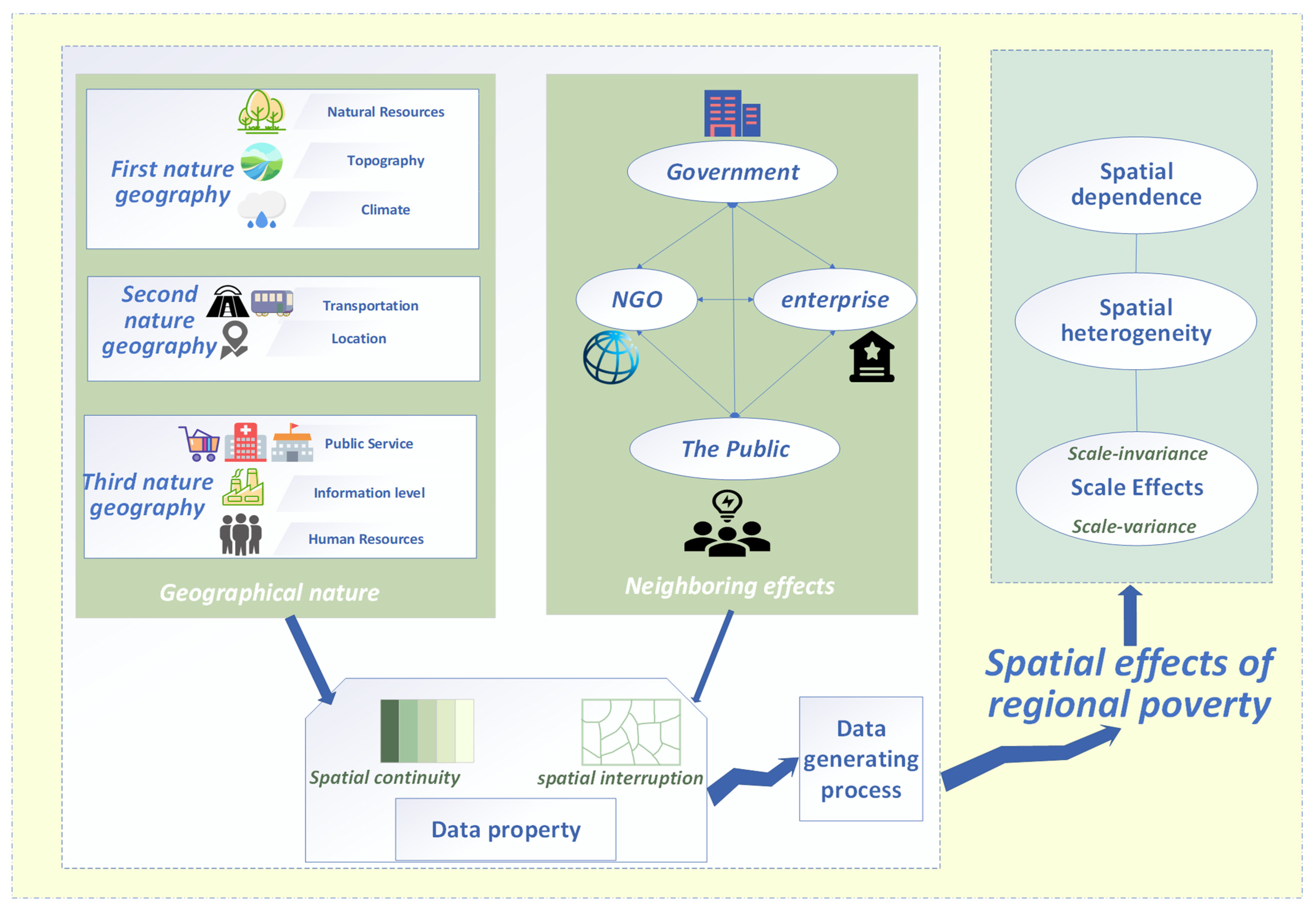
Figure 3.
Variation in LISA of regional poverty at different levels.

Figure 4.
Relative importance of geographical variables explaining poverty at different levels (metrics first normalized to add up to 100% and then multiplied by the adjusted R2 to represent their real contribution at each scale).
Figure 4.
Relative importance of geographical variables explaining poverty at different levels (metrics first normalized to add up to 100% and then multiplied by the adjusted R2 to represent their real contribution at each scale).
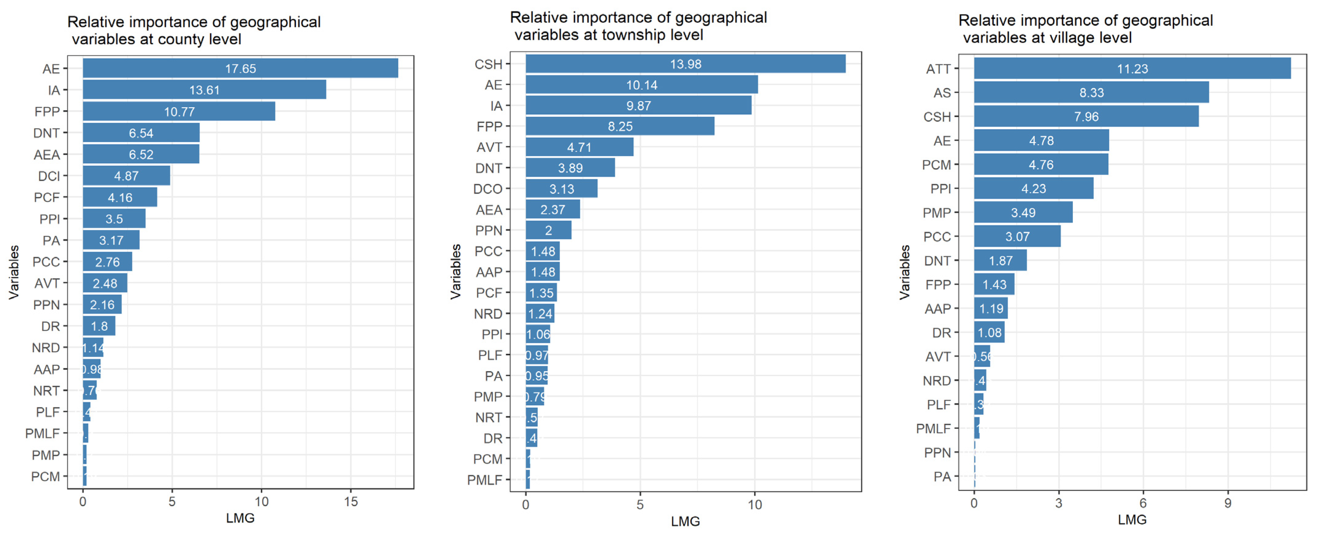
Figure 5.
Bivariate relations between poverty incidence and individual significant geographical factors.
Figure 5.
Bivariate relations between poverty incidence and individual significant geographical factors.
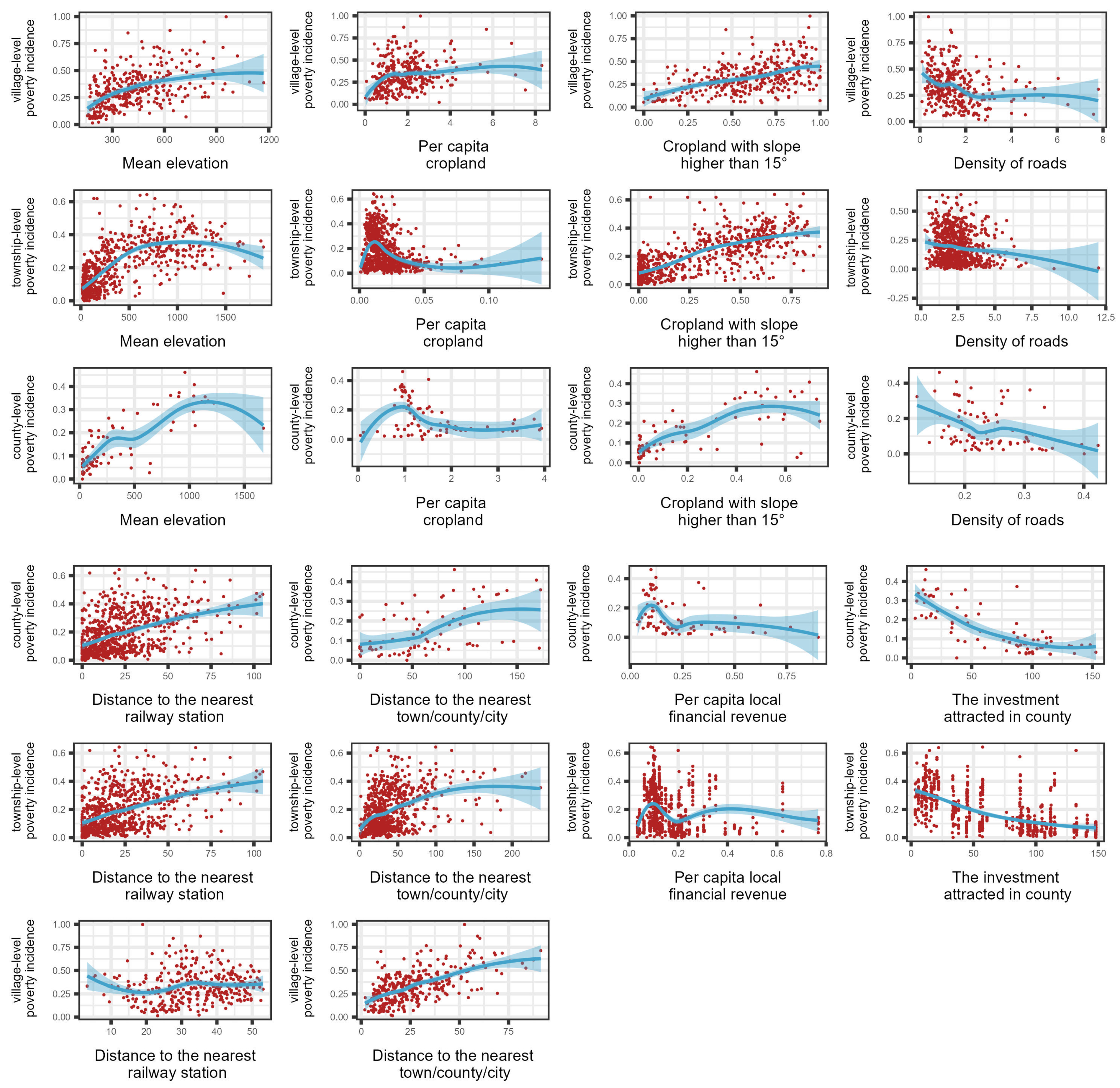
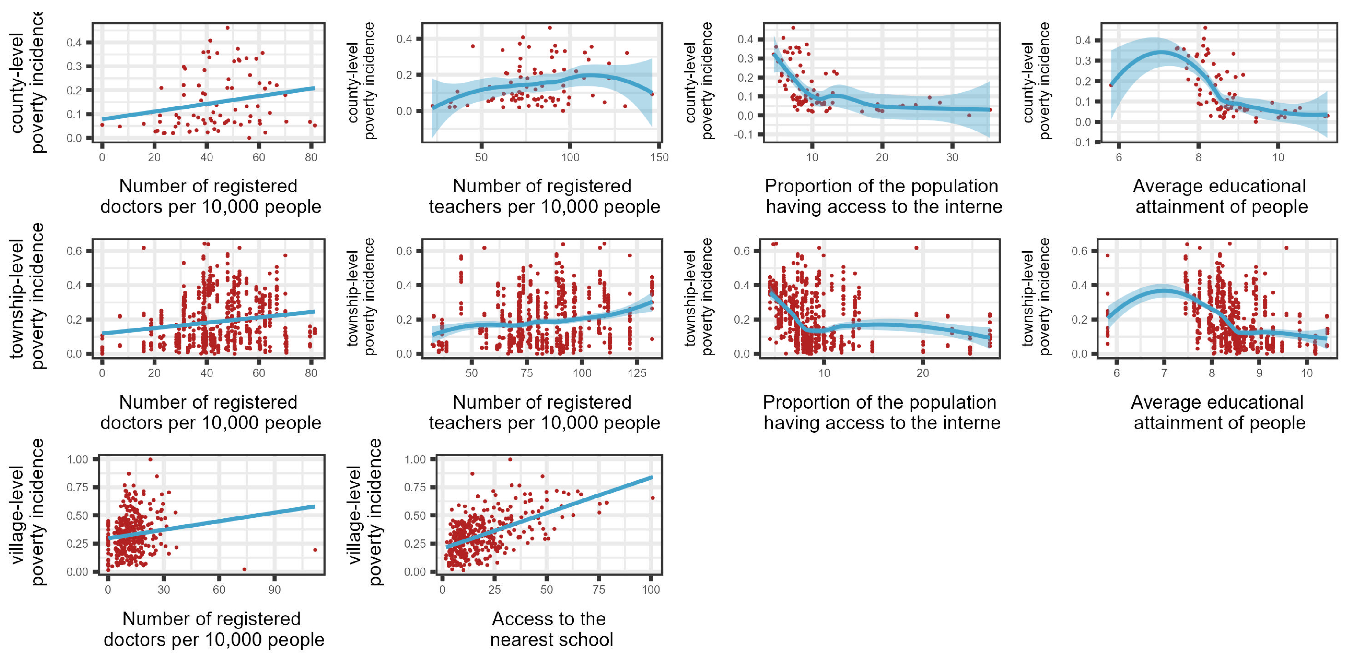
Figure 6.
Ranges of the regression coefficient of different geographical factors in MGWR models at different scales.
Figure 6.
Ranges of the regression coefficient of different geographical factors in MGWR models at different scales.
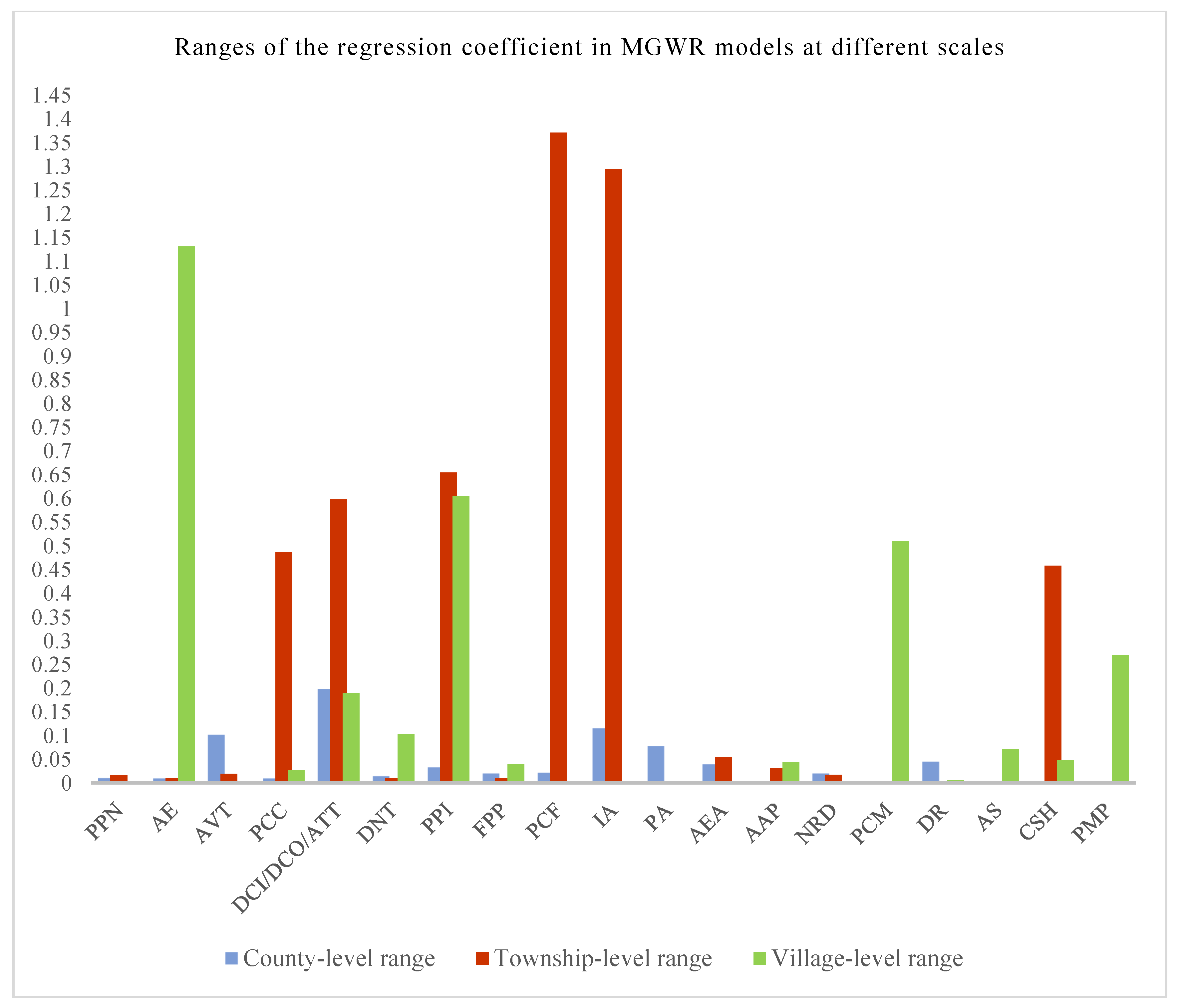
Figure 7.
Local estimates for (a) average elevation, (b) distance to the nearest administrative center, (c) proportion of the population having access to the internet at different levels.
Figure 7.
Local estimates for (a) average elevation, (b) distance to the nearest administrative center, (c) proportion of the population having access to the internet at different levels.
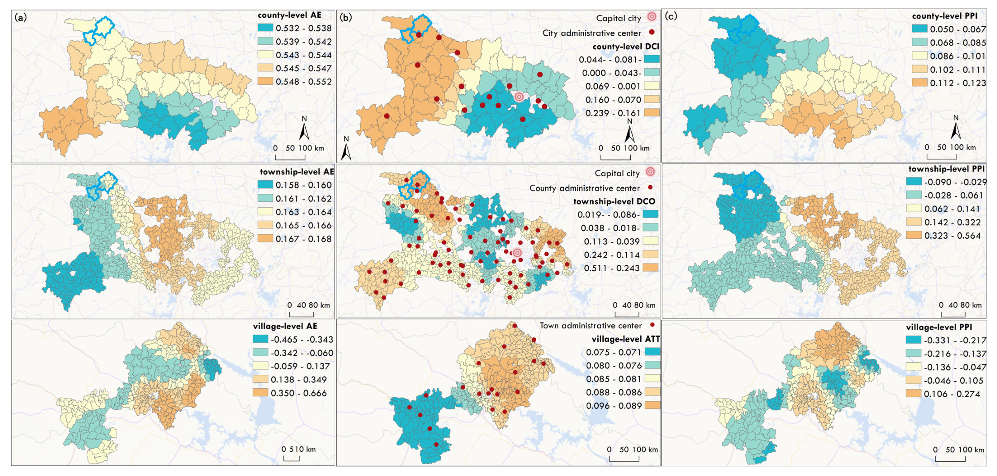
Table 2.
Results of the spatial autocorrelation analysis of poverty incidence at different levels in Hubei Province.
Table 2.
Results of the spatial autocorrelation analysis of poverty incidence at different levels in Hubei Province.
| County Level | Township Level | Village Level | |
|---|---|---|---|
| Moran’s Index | 0.67 *** | 0.66 *** | 0.44 *** |
| Variance | 0.071 | 0.019 | 0.001 |
| Z-score | 9.67 | 35.33 | 12.73 |
*** for p-value < 1 × 10⁻³, ** for < 1 × 10⁻² and * for < 5 × 10⁻¹.
Table 3.
Interpretation accuracy of the multi-linear model constructed between poverty incidence and geographical factors at different levels.
Table 3.
Interpretation accuracy of the multi-linear model constructed between poverty incidence and geographical factors at different levels.
| County Level | Township Level | Village Level | |
|---|---|---|---|
| Adjusted R2 | 0.84 | 0.69 | 0.55 |
| RMSE | 3.93 | 0.076 | 0.11 |
| F-statistic | 22.43 *** | 85.2 *** | 23.87 *** |
*** for p-value < 1 × 10⁻³, ** for < 1 × 10⁻² and * for < 5 × 10⁻¹.
Table 4.
Spearman’s correlation coefficient between poverty and geographical variables at different levels.
Table 4.
Spearman’s correlation coefficient between poverty and geographical variables at different levels.
| Administrative Levels | Administrative Levels | ||||||
|---|---|---|---|---|---|---|---|
| Variable | County (n = 91) | Township (n = 770) | Village (n = 341) | Variable | County (n = 91) | Township (n = 770) | Village (n = 341) |
| PPN | 0.615 *** | 0.552 *** | 0.058 | PLF | 0.132 | 0.071 | 0.045 |
| AE | 0.739 *** | 0.719 *** | 0.484 *** | PA | 0.459 *** | 0.239 *** | 0.086 |
| AVT | −0.306 ** | −0.428 *** | 0.027 | PMLF | −0.015 | 0.003 | 0.071 |
| AAP | 0.012 | −0.138 *** | 0.073 | PMP | −0.016 | −0.169 *** | 0.285 *** |
| PCC | −0.276 * | −0.295 *** | 0.285 *** | NRD | 0.263 * | 0.196 *** | 0.240 *** |
| FPP | −0.689 *** | −0.676 *** | 0.279 | NRT | 0.240 * | 0.199 *** | (AS) 0.508 *** |
| PCM | 0.367 *** | 0.018 | 0.379 *** | PPI | −0.647 *** | −0.401 *** | −0.450 *** |
| CSH | 0.720 *** | 0.729 *** | 0.487 *** | IA | −0.741 *** | −0.667 *** | |
| DR | −0.386 *** | −0.122 *** | −0.265 *** | AEA | −0.690 *** | −0.474 *** | |
| DNT | 0.518 *** | 0.441 *** | 0.190 *** | PCF | −0.498 *** | −0.204 *** | |
| DCI/DCO/ATT | 0.539 *** | 0.367 *** | 0.569 *** | ||||
*** for p-value < 1 × 10⁻³, ** for < 1 × 10⁻² and * for < 5 × 10⁻¹.
Table 5.
Variation in the impacts of geographical factor on poverty at different levels.
| Administrative Level | Overall Contribution (%) | First Nature Geography | Second Nature Geography | Third Nature Geography | ||||
|---|---|---|---|---|---|---|---|---|
| Physical Condition | Natural Endowments | Geolocation and Transportation | Governance Capability | Informatization Level | Public Service | Human Resources | ||
| County level | 84 | 23.27 | 13.72 | 13.21 | 17.77 | 3.5 | 2.1 | 10.4 |
| Township level | 69 | 18.33 | 23.9 | 7.51 | 11.22 | 1.06 | 2.55 | 4.46 |
| Village level | 55 | 6.57 | 17.22 | 14.18 | 0 | 4.23 | 12.25 | 0.54 |
Table 6.
Results of the spatial autocorrelation analysis of model residuals.
| County | Township | Village | |
|---|---|---|---|
| Moran’s Index | −0.0692 | 0.228 | 0.0580 |
| Expected Index | −0.0122 | −0.0013 | −0.0030 |
| Variance | 0.0738 | 0.0246 | 0.0338 |
| Z-score | −0.7785 | 9.2885 | 1.777 |
Table 7.
Results of the MGWR models at different levels in Hubei Province.
| County Level | Township Level | Village Level | |
|---|---|---|---|
| Adjusted R2 | 0.90 | 0.81 | 0.65 |
| Residual sum of squares | 5.23 | 124.23 | 104.11 |
Table 8.
Estimation result of MGWR models at different levels in Hubei Province.
| County Level | Township Level | Village Level | ||||
|---|---|---|---|---|---|---|
| Variable | Mean | Bandwidth | Mean | Bandwidth | Mean | Bandwidth |
| PPN | −0.186 | 89 | −0.047 | 768 | - | - |
| AE | 0.543 | 89 | 0.163 | 768 | 0.087 | 58 |
| AVT | −0.076 | 89 | −0.101 | 768 | - | - |
| PCC | 0.065 | 89 | 0.188 | 154 | 0.179 | 346 |
| DCI/DCO/ATT | 0.094 | 52 | 0.092 | 109 | 0.153 | 179 |
| DNT | 0.094 | 89 | 0.148 | 768 | −0.001 | 346 |
| PPI | 0.09 | 89 | 0.122 | 252 | −0.077 | 79 |
| FPP | −0.067 | 89 | −0.046 | 768 | −0.122 | 346 |
| PCF | −0.105 | 89 | −0.001 | 46 | - | - |
| IA | −0.28 | 54 | −0.348 | 44 | - | - |
| PA | −0.019 | 73 | - | - | ||
| AEA | −0.181 | 89 | −0.058 | 732 | - | - |
| AAP | - | - | 0.007 | 768 | 0.078 | 346 |
| NRD | 0.006 | 89 | 0.014 | 768 | - | - |
| PCM | - | - | - | - | 0.218 | 186 |
| DR | −0.026 | 77 | - | - | −0.008 | 346 |
| AS | - | - | - | - | 0.186 | 346 |
| CSH | - | - | 0.312 | 146 | 0.142 | 346 |
| PMP | - | - | - | - | 0.219 | 268 |
- representing that this factor was excluded in the MGWR model because it was not identified as important by LMG value (contribution less than 1%).
Disclaimer/Publisher’s Note: The statements, opinions and data contained in all publications are solely those of the individual author(s) and contributor(s) and not of MDPI and/or the editor(s). MDPI and/or the editor(s) disclaim responsibility for any injury to people or property resulting from any ideas, methods, instructions or products referred to in the content. |
© 2023 by the authors. Licensee MDPI, Basel, Switzerland. This article is an open access article distributed under the terms and conditions of the Creative Commons Attribution (CC BY) license (https://creativecommons.org/licenses/by/4.0/).
Share and Cite
MDPI and ACS Style
Liu, M.; Ge, Y.; Hu, S.; Hao, H. The Spatial Effects of Regional Poverty: Spatial Dependence, Spatial Heterogeneity and Scale Effects. ISPRS Int. J. Geo-Inf. 2023, 12, 501. https://doi.org/10.3390/ijgi12120501
AMA Style
Liu M, Ge Y, Hu S, Hao H. The Spatial Effects of Regional Poverty: Spatial Dependence, Spatial Heterogeneity and Scale Effects. ISPRS International Journal of Geo-Information. 2023; 12(12):501. https://doi.org/10.3390/ijgi12120501
Chicago/Turabian StyleLiu, Mengxiao, Yong Ge, Shan Hu, and Haiguang Hao. 2023. "The Spatial Effects of Regional Poverty: Spatial Dependence, Spatial Heterogeneity and Scale Effects" ISPRS International Journal of Geo-Information 12, no. 12: 501. https://doi.org/10.3390/ijgi12120501
Note that from the first issue of 2016, this journal uses article numbers instead of page numbers. See further details here.