Variability of Extreme Climate Events and Prediction of Land Cover Change and Future Climate Change Effects on the Streamflow in Southeast Queensland, Australia

Abstract

The severity and frequency of extremes are changing; thus, it is becoming necessary to evaluate the impacts of land cover changes and urbanisation along with climate change. A framework of the Generalised Extreme Value (GEV) method, Google Earth Engine (GEE), and land cover patterns’ classification including Random Forest (RF) and Support Vector Machine (SVM) can be useful for streamflow impact analysis. For this study, we developed a unique framework consisting of a hydrological model in line with the Process-informed Nonstationary Extreme Value Analysis (ProNEVA) GEV model and an ensemble of General Circulation Models (GCMs), mapping land cover patterns using classification methods within the GEE platform. We applied these methods in Southeast Queensland (SEQ) to analyse the maximum instantaneous floods in non-stationary catchment conditions, considering the physical system in terms of cause and effect. Independent variables (DEM, population, slope, roads, and distance from roads) and an integrated RF, SVM methodology were utilised as spatial maps to predict their influences on land cover changes for the near and far future. The results indicated that physical factors significantly influence the layout of landscapes. First, the values of projected evapotranspiration and rainfall were extracted from the multi-model ensemble to investigate the eight GCMs under two climate change scenarios (RCP4.5 and RCP8.5). The AWBM hydrological model was calibrated with daily streamflow and applied to generate historical runoff for 1990–2010. Runoff was projected under two scenarios for eight GCMs and by incorporating the percentage of each land cover into the hydrological model for two horizons (2020–2065 and 2066–2085). Following that, the ProNEVA model was used to calculate the frequency and magnitude of runoff extremes across the parameter space. The maximum peak flood differences under the RCP4.5 and RCP8.5 scenarios were 16.90% and 15.18%, respectively. The outcomes of this study suggested that neglecting the non-stationary assumption in flood frequency can lead to underestimating the amounts that can lead to more risks for the related hydraulic structures. This framework is adaptable to various geographical regions to estimate extreme conditions, offering valuable insights for infrastructure design, planning, risk assessment, and the sustainable management of future water resources in the context of long-term water management plans.

1. Introduction

The Intergovernmental Panel on Climate Change Assessment Report (IPCC) [1,2] on climate change indicates that climate change will be accompanied by a rise in the frequency, severity, and duration of extreme natural phenomena such as excessive precipitation and extreme air temperatures in the twenty-first century. The trends suggest that the frequency and intensity of flood events are likely to rise globally due to climate and land use/cover changes attributed largely to urbanisation and anthropogenic activities [2,3]. Ding et al. [4] claimed that one of climate change’s most significant implications is the increased frequency and occurrence of severe weather conditions. As hydrological events are more prone to be frequent and extreme, it is becoming increasingly crucial to assess how hydrological events respond to future land use and climate conditions [5]. During extremes, an efficient and economical strategy for achieving situational awareness is essential to enhancing the management of emergency responses. The ability to forecast the occurrence and scale of extreme events is crucial for both infrastructure and emergency management.

Climates are tremendously changeable from year to year at various locations across the world, including Australia, the world’s driest inhabited continent, where there is a diverse range of climatic regimes, making it more vulnerable to climate change [6]. According to research [7,8], projected changes in the climate are anticipated to have noticeable effects on the frequency of hydrological elements such as runoff, rainfall, and evapotranspiration (ET) across various regions. Distinguishing between the effects of climate changes and land use changes on observed hydrological shifts is often challenging due to their concurrent occurrence in most regions, with both climate change and land use alterations [8,9]. So, a framework that incorporates land cover patterns and an ensemble of GCMs can be helpful.

Extreme hydrological events have been seen to be significantly influenced by climate change [10] and land cover changes caused by human activities. It is widely acknowledged that climate projections and scenarios, especially concerning extreme events, including extreme precipitation [11] and extreme streamflow, exhibit significant uncertainty across many global regions. Research on hydrological extremes is critically needed, especially for locations where the consequences of climate change are known to be significant [12].

Stationarity was previously believed to make complex statistical studies simpler, as studied by [13]. It offered significant insights into planning, making choices, and comprehending the effects of climate events, assuming a stable climate. Longer data records and a changing environment, however, make assuming stationarity riskier than ever. Under the assumption of a stationary climate, the terms return a level return duration and provide crucial information for decision making, design, and evaluating the effects of outstanding meteorological and climatic events. Traditionally, infrastructure design methods relied on the assumption of constant return levels, assuming that the occurrence of extreme events remains consistent over time [14]. However, it has become evident that the frequency of extreme events is evolving and is anticipated to keep changing in the future [1] Research has also revealed that non-stationarity in hydrological records in certain regions is characterised by increasing or decreasing patterns [13]. Since many extremes include spatial information, the major focus of recent framework advancements has been the challenge of combining spatial information with extreme value analysis strategies [15,16]. Therefore, models capable of accommodating non-stationary climatic and hydrologic extremes are essential [17,18].

Land use/cover changes (LUCC) have been identified as another influential factor for changing hydrological regimes [5]. It should be highlighted that the majority of research on LUCC is based on historical land use statistics [19] and has paid less attention to the linked effects of land cover changes and climate change. Therefore, it is important to estimate future land use scenarios and determine their impacts on extreme hydrological events. In the realm of land cover management and planning, two machine learning algorithm models are employed in Google Earth Engine (GEE): Random Forest (RF) [20] and Support Vector Machine (SVM) [21].

The prolonged presence of extremes poses detrimental impacts on infrastructure, the economy, and human health [22,23,24,25,26]. Applying Nonstationary Extreme Value Analysis (NEVA) [14] grounded in Bayesian inference could identify design extremes at various recurrence durations and intervals by performing a frequency analysis of extremes, observing alterations in the return period [27].

Various statistical distributions, such as Generalized Extreme Value (GEV) distributions [28], find extensive application in the examination of the intensity and frequency of extreme events within climate and hydrology research. Moreover, it has been recommended by the Australian Rainfall and Runoff (ARR) guideline [29] that the GEV distribution be utilized for estimating extreme floods and rainfalls.

Thus, in this research, streamflow is considered based on stationary and non-stationary assumptions. This study assesses the streamflow characteristics in the Lockyer catchment of southeastern Queensland, Australia, to establish return levels. The study aims to develop a methodology and identify the integrated effects of land cover and climate change on extreme streamflow events. The objective of the research is to accomplish the following specific objectives: (1) to explore a methodology that integrates a hydrological model with ensembles of Global Climate Models (GCMs) under Representative Concentration Pathways (RCPs) and projected landcover scenarios along with GEV to improve extremes predictions under the instantaneous impacts of climate change and human activities; (2) applying SVM and RF classification in GEE for projecting future land cover changes; (3) investigating the trend of land cover changes in the basin and projecting these changes with ensembles of GCMs under RCPs for future horizons; (4) performing hydrological simulations for each landcover classification separately under climatic scenarios and landcover changes at baseline and for near and far future horizons; and (5) to apply the ProNEVA model [28], which analyses and compares the return levels of projected streamflow under stationary and non-stationary assumptions and maps the spatiotemporal distribution of extreme events.

More work should be put into adding crucial physical processes to stochastic models, according to [30], who also recommended stochastic-process-based models as a means to bridge the gap between physically based models and statistical models. In this study, we propose an integrated framework for assessing the past and future hydrological consequences of climate change. This framework integrates hydrological models, a machine learning method on the GEE platform, ProNEVA, and climate projections under different scenarios based on the Generalised Extreme Value (GEV) model in stationary and non-stationary conditions [13] and explores the effects of future climate change on the streamflow. Firstly, we presented a technique for obtaining and evaluating the remotely sensed temporal imagery [8] necessary for incorporating land cover into hydrological modelling. Secondly, we assessed the outputs of the GCMs under RCPs projecting the futurist climate simulations that were included in the hydrological model, as recommended by [8,31]. Thirdly, we applied SVM and RF classification in the GEE platform for projecting future land cover changes. Lastly, we applied the ProNEVA model to estimate return levels and assess the frequency and severity of extreme events in streamflow under both assumptions, including non-stationary and stationary. This study’s findings will contribute to our knowledge of how severe flood events vary spatially at the catchment level. Investigations into adaptation techniques for handling probable future extremes will be assisted by this new framework for water planners and decision makers.

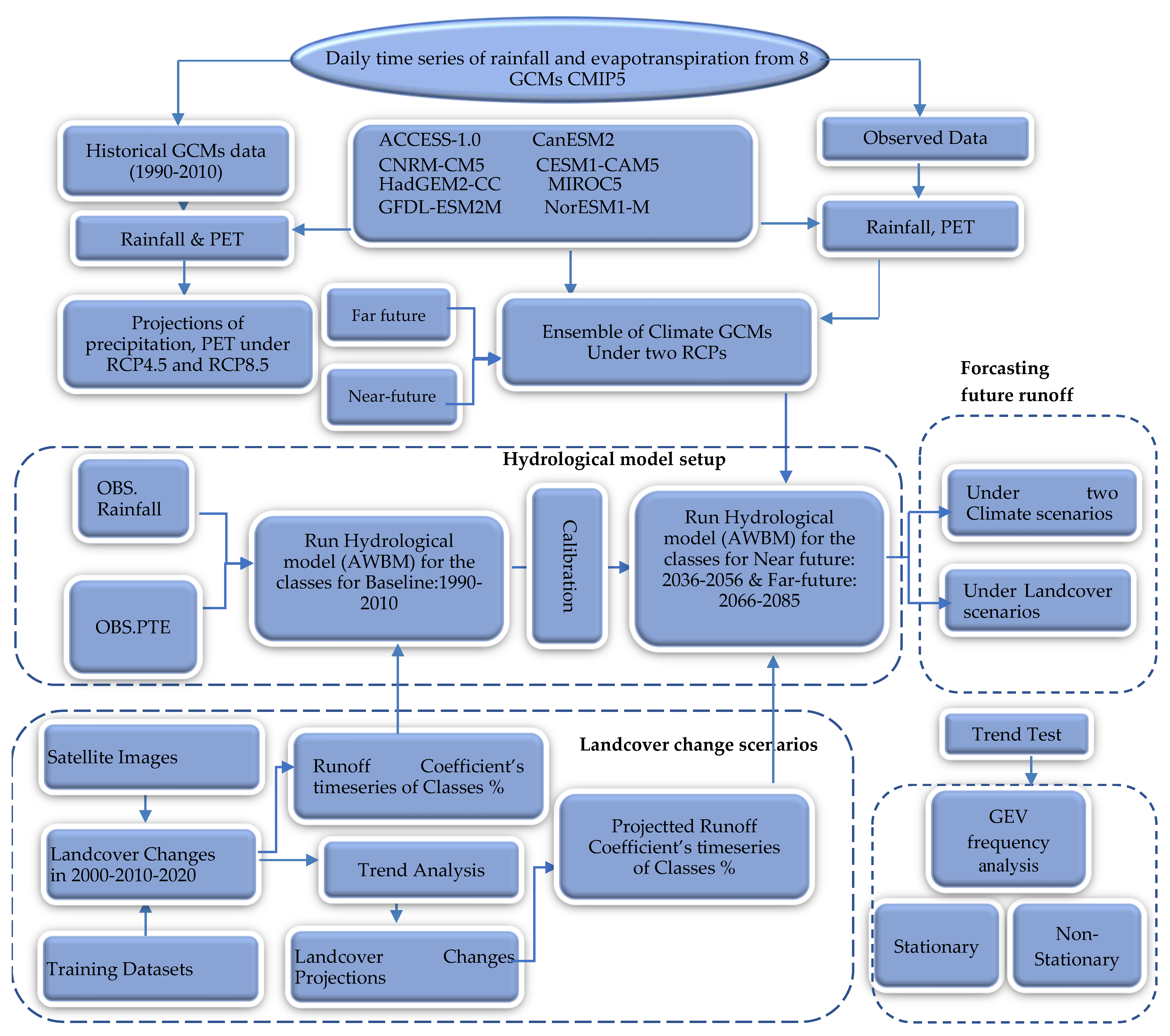
2. Materials and Methods

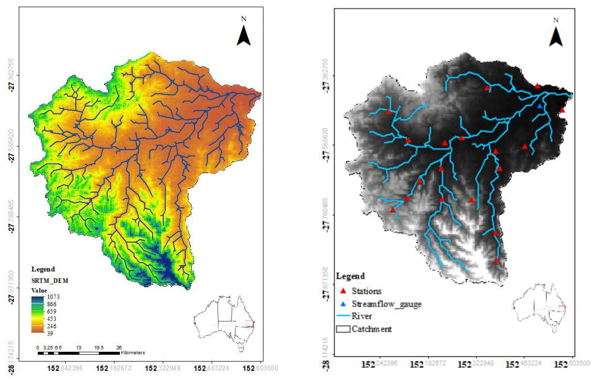
The primary techniques and data employed in this investigation are depicted in Figure 1. The procedures outlined in this study are as follows: (a) gaining projected climate variables (rainfall and potential ET) derived from a GCM obtained from the Coupled Model Intercomparison Project Phase 5 (CMIP5) to evaluate climate change impacts on the study area for historical and future periods, (b) calibrating and validating a hydrologic model to analyse the changes in daily inflows that will be used for the streamflow projection, (c) applying SVM and RF classification in GEE for projecting future land cover changes, (d) deriving the runoff coefficient’s time series of classes (%) from historical LandSat images and for the near and far future, and (e) evaluating the extremes analysis applying the GEV model.

2.1. Study Area

The case study region, Lockyer Catchment, is situated in SEQ, as shown in Figure 2. Lockyer Creek, a tributary of Brisbane River, is the primary stream, surrounded by several sub-catchments. The catchment covers an area of 3000 km², experiencing an average annual rainfall ranging from 1000 to 2012 mm [32]. The Lockyer catchment includes a range of physical geographic attributes, encompassing the distance of water paths from 0 to 102,815 m, elevations ranging between 30 and 1073 m, basin slopes spanning from 0 to 66 degrees, channel network slopes ranging from 0 to 18 degrees, and a total channel network length of 922,025.285 m. The Lockyer catchment provides significant environmental, economic, and social values and Australia’s most fertile agricultural land for the cultivation of highly valuable vegetables [33]. In Australia, floods are one of the frequently occurring disasters that have accounted for substantial amounts of environmental and economic losses in recent years; hence, mitigation of the risks associated with the impacts of these events is necessary [34,35].

There have been a number of exceptional weather occurrences in this area in recent years. For example, in December 2010 and January 2011, continuous rains caused unprecedented levels of flooding to spread throughout significant regions of Queensland [34]. A disaster zone was designated across 78% of the state due to the detrimental impact on 2.5 million people. Over 29,000 houses and businesses were impacted by the floods, which are believed to have caused damage worth over AUD 5 billion [34].

Given that past research has proven the assumption of stationary to be no longer accurate, the frequency of flood occurrences, like the one in February 2022, demonstrates that this assumption is no longer applicable. Furthermore, it has been noted that the connection between runoff and rainfall in this catchment is not constant over time [36,37]. In addition, investigating the impacts of land cover changes and climate change on the streamflow is important. To improve the design and management of hydraulic infrastructure and reduce future human and financial losses, it is imperative to develop unique approaches for estimating non-stationary runoff extremes [13].

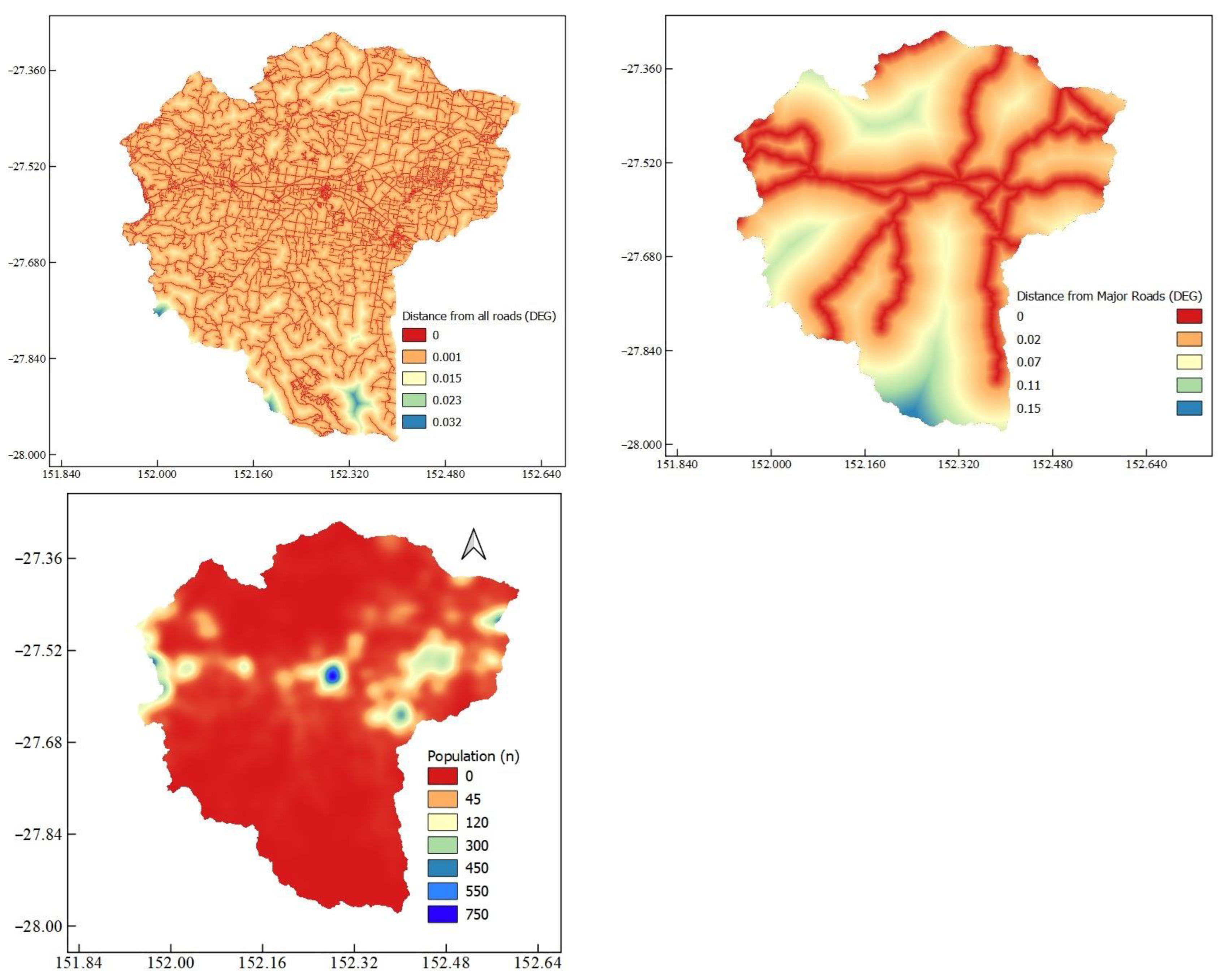
2.2. Data Sources: Observed, Remotely Sensed Data and Geospatial Data

Daily hydrological data, including potential evapotranspiration (mm) and rainfall (mm), were retrieved from the stations. The 5 km grid data were achieved through SILO, an Australian climate data source (http://www.longpaddock.qld.gov.au/silo (accessed on 15 January 2023)) [38,39], and cover the period from 1990–2005. Important rainfall sites were selected because of their geographic variety and data quality, which comprised long records with few missing values. Daily streamflow records for 143210B Lockyer Creek at Rifle Range Road station were received from the Queensland Government Water Monitoring Information site (https://water-monitoring.information.qld.gov.au/ (accessed on 15 January 2023)).

The Landsat satellite images (from TM, ETM+, and OLI 1&2 sensors) and ESA global land cover dataset were accessed and used through GEE [40] for conducting the classifications and modelling of changes in land cover and urban growth. Geospatial datasets of road networks, population density, and the Hydrologically Enforced Digital Elevation Model (DEM-H) product with a 30 m spatial resolution [41] dataset were used as supplementary data inputs during the landcover projection analysis. Since the distance from roads and population density maps were originally in vector format, both maps were first converted into the raster format, resampled to the 30 m spatial resolution, and used for the projection of landcover changes (

Table 1. Sources of datasets.

Raster Dataset	Time Coverage	Data Source	Resolution/ Format
Landsat 5 TM	2000–2011	Google Earth Engine (LANDSAT/LT05/C02/T1_L2)	30 m
Landsat 8 OLI	2013–2023	Google Earth Engine (LANDSAT/LT08/C02/T1_L2)	30 m
ESA global land cover	2021	Google Earth Engine (ESA/WorldCover/v100)	10 m
DEM-H: Australian SRTM Hydrologically Enforced Digital Elevation Model	2010	Google Earth Engine (AU/GA/DEM_1SEC/v10/DEM-H)	30 m
Vector Dataset		Source	Data Format
Roads	2000 and 2023	Queensland Government	Shapefile (.shp)
Distance from roads	2023	Spatial analysis on road network	Shapefile (.shp)
Population	2023	Australian Bureau of Statistics	Shapefile (.shp)

).

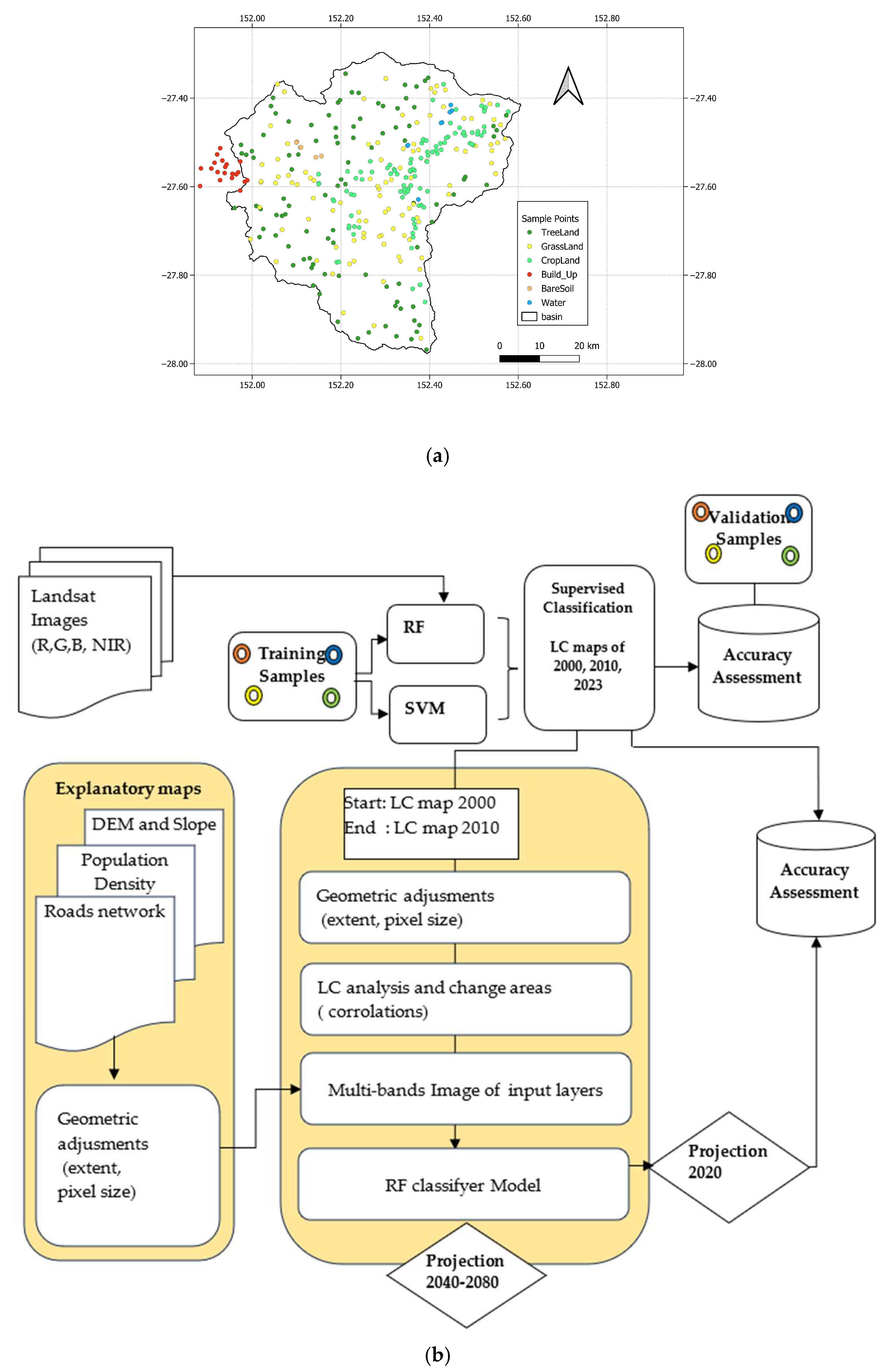
2.3. Classification and Projection of Landcover Changes

To project the landcover changes, first, the main land cover types were classified into six classes (

Table 2. Land cover classification scheme.

Land Cover Type	Description
Tree cover	Forest and tree cover land
Grassland	Pastures, green spaces, parks, and bushlands
Cropland	Farmland, agricultural
Built-up	Built-up area, residential, commercial, and other infrastructure
Bare/sparse vegetation	Bare soils, sand, rocks, and sparse vegetation
Water Bodies	Lakes, ponds, reservoirs, and rivers

), and, following ESA global landcover classification [42], discriminated from other features in the Landsat images for the years 2000, 2010, and 2020 using two supervised classification models, including Support Vector Machine (SVM) and Random Forests (RF). The image collection of Landsat images was called for the years 2000, 2010, and 2020 in GEE, separately. The images were filtered based on criteria related to cloud conditions and vegetation cover. The remaining images in each collection were reduced to a single multiband images using median reducers.

To train the classification models, we mapped the boundaries of more than 200 point features (335) representing six different classes: tree cover, grassland, cropland, built-up, bare soil/sparse vegetation, and water bodies using ESA global landcover and drawing geometry tools in GEE. The training datasets were split up into groups for training and validation. In total, 70% of the point features were assigned to the training and 30 percent were used in the validation procedure.

The spatial distribution of both the training and validation polygons is illustrated in Figure 3a. After generating the landcovers for the years 2000, 2010, and 2020, the landcover changes were simulated and projected using the SVM and RF approaches in the GEE platform, which is shown in Figure 3b.

2.3.1. SVM Classification

SVM is one of the most reliable and widely applied supervised nonparametric statistical machine learning techniques [43,44]. To discriminate between various categories, the SVM method translates the training data into two-dimensional space and fits the best hyperplane. The kernel functions, which are non-linear mapping functions, are used to define the optimal hyperplane, which divides the classes. The SVM module [45] is employed for training and classification, utilising a radial basis function (RBF) kernel. Moreover, a radial basis function is characterised by its computational speed and straightforward implementation, involving the tuning of two parameters. These parameters include cost ‘sigma (C)’, a substantial value used to fine-tune the error associated with misclassifying instances in the training dataset, and ‘gamma (γ)’, which represents the kernel width.

2.3.2. RF Classification

A non-parametric machine learning method called Random Forest (RF) [20] was created based on the idea of a learning strategy. To create a single classification, RF combines many tree-based classifiers into an ensemble of decision trees, where each tree provides a vote to choose which class should be assigned to the input data [45,46,47].

2.3.3. Landcover Changes Projection

The probability of transitions from the RF learning procedure is employed in this work to characterise the changes in land cover. Land cover maps for the starting year (2000) and the finishing year (2010) are included in the model’s first phase. After importing the spatial variable factors, such as DEM, population density, and distance from the road, into the model, a land cover change map is produced, from which the research area’s changing pattern between 2000 and 2010 is established (Figure 3). The properties of the explanatory maps are extracted in the same raster format for all datasets, with the exact geographical projected coordinates of EPSG 4326 and a resolution pixel size of 0.000269495 degrees.

To project the changes in land cover, a script was written in GEE to calculate the percentage of area changes in a given year. It generates a transition matrix that shows the proportion of pixels shifting from one land cover to another. The code also creates an area change map that shows the changes in the land between 2000 and 2010 for all six classes: tree cover, grassland, cropland, built-up, bare soil, and water bodies.

The future land cover maps are predicted assuming that existing land cover patterns and dynamics are continuing. Also, based on the classified raster images of 2000 and 2010, land cover transitions are predicted for 2040 and 2060. To model the land cover forecast, the RF and SVM classification techniques were used to forecast the land cover map.

2.3.4. Accuracy Assessment

Several statistical indicators were used to evaluate the classified maps, including the Kappa coefficient, User’s Accuracy (UA), Producer’s Accuracy (PA), and Overall Accuracy (OA). The amount of properly identified pixels in a given class divided by the total number of classified pixels in the class is known as the UA. The Kappa coefficient quantifies the level of agreement between the classification map generated by remote sensing and the reference data. Meanwhile, the OA is determined by the ratio of pixels correctly classified to the total number of pixels.

2.4. Hydrological Model

Most hydrological models were developed as tools in water management, particularly for providing climatic and weather conditions in relation to river flow and available water [48,49,50,51]. The Australian Water Balance Model (AWBM) was created in the 1990s [52,53,54] and has been used in other countries, becoming one of Australia’s most extensively used hydrological models [53,55,56]. The Rainfall-Runoff Library (RRL) is freely available for users (further information is available at (https://toolkit.ewater.org.au/Tools/RRL (accessed on 15 January 2023)). Yu and Zhu [57] indicated that the AWBM is better for simulating climate-driven fluctuations in observed streamflow and characterising the consequences of precipitation changes. The concept of selecting an appropriate hydrological model has been proven by Jahandideh-Tehrani, et al. [58], as in the Australian region, lumped conceptual hydrological models [59] such as the AWBM are well-suited to use for runoff simulation. The AWBM was created to minimise problems related to physically based hydrological models such as different parameter estimations. For the study catchment, the AWBM model was calibrated at the daily time step. For simulation purposes, calibration (60%) and validation (40%) were employed. The availability of recorded runoff data determined the calibration and validation timeframes for the Lockyer catchment. So, runoff data were used for 1990–2002 (calibration period) and 2003–2010 (for validation period). Daily rainfall, potential ET (PET), and daily runoff were derived from SILO and WMIP throughout the catchment, respectively (Section 2.2).

The AWBM [60] structure and parameters are presented in

Table 3. Description of parameter values for the AWBM model [60].

Parameter ID	Description	Unit	Default	Minimum	Maximum
A1	Partial area represented by surface storage	-	0.134	0	1
A2		-	0.433	0	1
BFI	Baseflow Index	-	0.35	0	1
C1	Surface storage capacities	mm	7	0	50
C2		mm	70	0	200
C3		mm	250	0	500
Ks	Surface flow recession constant	-	0.90	0	1
Kb	Baseflow recession constant	-	0.90	0	1

. The AWBM is mostly made up of three basic surface storage configurations. The depths of these storage tanks are equal to the C1, C2, and C3 (three surface moisture stores) parameters to create the coefficient of runoff simulation. For each time step, the water balance of each partial region is determined [61]. As demonstrated by [8], in this study, runoff from impermeable surfaces was taken into account by recoding and changing the AWBM. The eight calibrated parameters are adjusted for accuracy in Table 3.

To analyse the impacts of climate change on runoff at various sizes, ranging from small locations to huge geographic areas, hydrological models have been widely implemented. The goal of this research is to estimate the effects of climate change on the streamflow in a major catchment (the Lockyer Creek catchment). To accomplish this, a rainfall–runoff model was adjusted and validated before being used to forecast runoff. So, the AWBM was undertaken to assess the impact of climate variability on runoff. The most vital step in climate change research is selecting climate models for future hydro-climatological projections.

The accuracy assessment of the models’ validation and calibration was performed based on statistical measurements [62,63], including the correlation coefficient (R²), Nash-Sutcliffe coefficient (E), Bias, and Root Mean Square Error (RMSE), as follows (Equations (1)–(4)):

$$R^2={\left(\frac{\frac{1{\sum }_1^n\left(X_{obs}-X_{obs}\right)\left(X_{sat}-X_{sat}\right)}{n}}{X_{obs}\times X_{sat}}\right)}^2$$

(1)

$$RMSE=\sqrt{\sum _1^n\frac{{\left(X_{sat}-X_{obs}\right)}^2}{n}}$$

(2)

$$\mathrm{B}\mathrm{i}\mathrm{a}\mathrm{s}=\frac{{\sum }_1^{\mathrm{n}}\left({\mathrm{X}}_{\mathrm{s}\mathrm{a}\mathrm{t}}-{\mathrm{X}}_{\mathrm{o}\mathrm{b}\mathrm{s}}\right)}{\mathrm{n}}$$

(3)

$$\mathrm{E}=1-\left(\frac{\frac{1{\sum }_1^n{\left(Q_{obs}-Q_{sim}\right)}^2}{n}}{\frac{1{\sum }_1^n{\left(Q_{obs}-\overline{Q_{obs}}\right)}^2}{n}}\right)$$

(4)

In which Q_obs and Q_sim show the observed and simulated time series, respectively; n is the total number of observations; and $\overline{Qobs}$ is the average of observational values.

2.5. Future Climate Projections and Greenhouse Gas Emissions Scenarios

The Coupled Model Intercomparison Project (CMIP) is the largest intercomparison study and it serves as a baseline for assessing GCMs’ capacity to project observed climate changes. In this study, climate change effects on the streamflow in the Lockyer catchment were assessed using eight GCMs of CMIP5. The recently suggested RCPs provide a broader range of possible futures by taking mitigation techniques and land use changes into account [38]. According to the aim of this research study, it is imperative to select appropriate RCP scenarios. RCP 8.5 scenarios [64], which represent high GHG scenarios, have been selected and are currently trending in the same direction, and RCP 4.5 is a depiction of a low-emission scenario and was chosen to analyse less severe situations.

Individual CMIP5 models’ capability to predict the Australian climate varies depending on whatever part of the modelling process is studied. These models are the most accurate instruments for predicting the reactions of regional climates in the twenty-first century [65]. Based on the third and fifth stages of the CMIP, Alexander and Arblaster [66] conducted detailed evaluations of anticipated changes in extreme climate events over Australia.

As mentioned in the climate change technical report in Australia [38], the Australian Water Availability Project (AWAP) observed temperature and rainfall data (https://eo-data.csiro.au/projects/awap/ (accessed on 15 January 2023)) were used to create climatic outputs with a resolution of 5 km. In this approach, the model data, whose resolution ranged from 100 to 310 km, were initially applied to the observed data using interpolation on a 5 km grid. In this research, according to the Australian climate change technical report [38], these eight climate models have been suggested for investigating climate change’s impacts on SEQ (

Table 4. List of eight CMIP5 models used in this research [38].

CMIP5 Model ID	Modelling Centre, Country of Origin, Institution	Ocean Resolution (°LAT × °LON)	Atmospheric Resolution (°LAT × °LON)
ACCESS-1.0	Commonwealth Scientific and Industrial Research Organisation, Partnership between CSIRO and BOM, Australia	1.0 × 1.0	1.9 × 1.2
CNRM-CM5	National Center for Meteorological Research, France	1.0 × 0.8	1.4 × 1.4
CESM1-CAM5	National Center for Atmospheric Research, National Science foundation, United States	1.1 × 0.6	1.2 × 0.9
CanESM2	Canadian Centre for Climate Modeling and Analysis, Canada	1.4 × 0.9	2.8 × 2.8
GFDL-ESM2M	Geophysical Fluid Dynamics Laboratory, United States	1.0 × 1.0	2.5 × 2.0
HadGEM2-CC	MOHC (Met Office Hadley Centre for Climate Science and Services, United Kingdom)	1.0 × 1.0	1.9 × 1.2
MIROC5	Centre for Climate System Research, Japan Atmosphere and the University of Tokyo Ocean Marine-Earth Science and Technology Research Institute	1.6 × 1.4	1.4 × 1.4
NorESM1-M	Norwegian Climate Center (NCC) and University of Bergen, Norway	1.1 × 0.6	2.5 × 1.9

).

2.6. Assessing Extremes in a Non-Stationary Approach Using the GEV Model

Non-stationary situations arise because the stationary assumption might not be valid for changes brought about by human and climate variables. Even with great progress [14], there is still no complete framework that incorporates the Extreme Value Analysis (EVA) statistical models (Generalised Extreme Value (GEV), Generalised Pareto (GP), and Log-Pearson type III (LP3)) under stationary and non-stationary assumptions (parameters as a function of physical variables or time) [28]. The ProNEVA (https://amir.eng.uci.edu/software.php (accessed on 15 January 2023)) software [28] was employed to examine non-stationary extremes.

With user-defined covariates, which may be time or a physical variable, ProNEVA enables non-stationary studies. The benefit of conducting a stationary analysis with covariates related to the physical aspect lies in the ability to incorporate physical limitations into a statistical model. ProNEVA employs a Bayesian approach to evaluating extremes, utilising a Differential Evolution Markov Chain methodology throughout the parameter value [14]. The essential distributions offered by Extreme Value Theory (EVT) to describe extremes are as follows: the use of Generalised Pareto Distribution (GPD) through the peaks-over-threshold approach [67,68,69], with the block maxima technique employing the LP3 and GEV family of distributions [70]. Additional details on the GEV distribution have been demonstrated in this article [13].

3. Results

The study establishes a multi-framework by the combination of a hydrological model in line with ProNEVA and an ensemble of GCMs under two RCPs, mapping land cover patterns by implementing the machine learning classification methods in GEE. With consideration for the physical components and how they interact with one another within the system, this integrated approach attempts to evaluate the return levels of flood extremes.

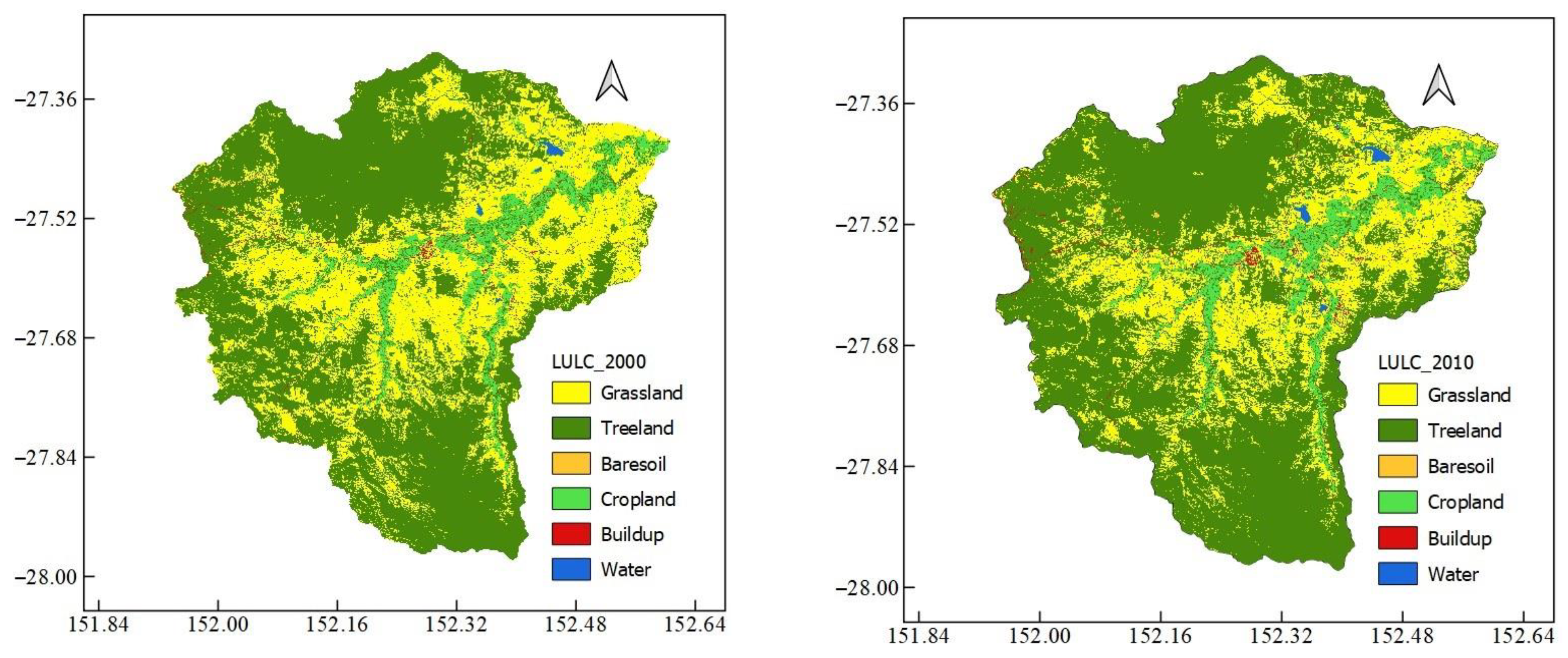
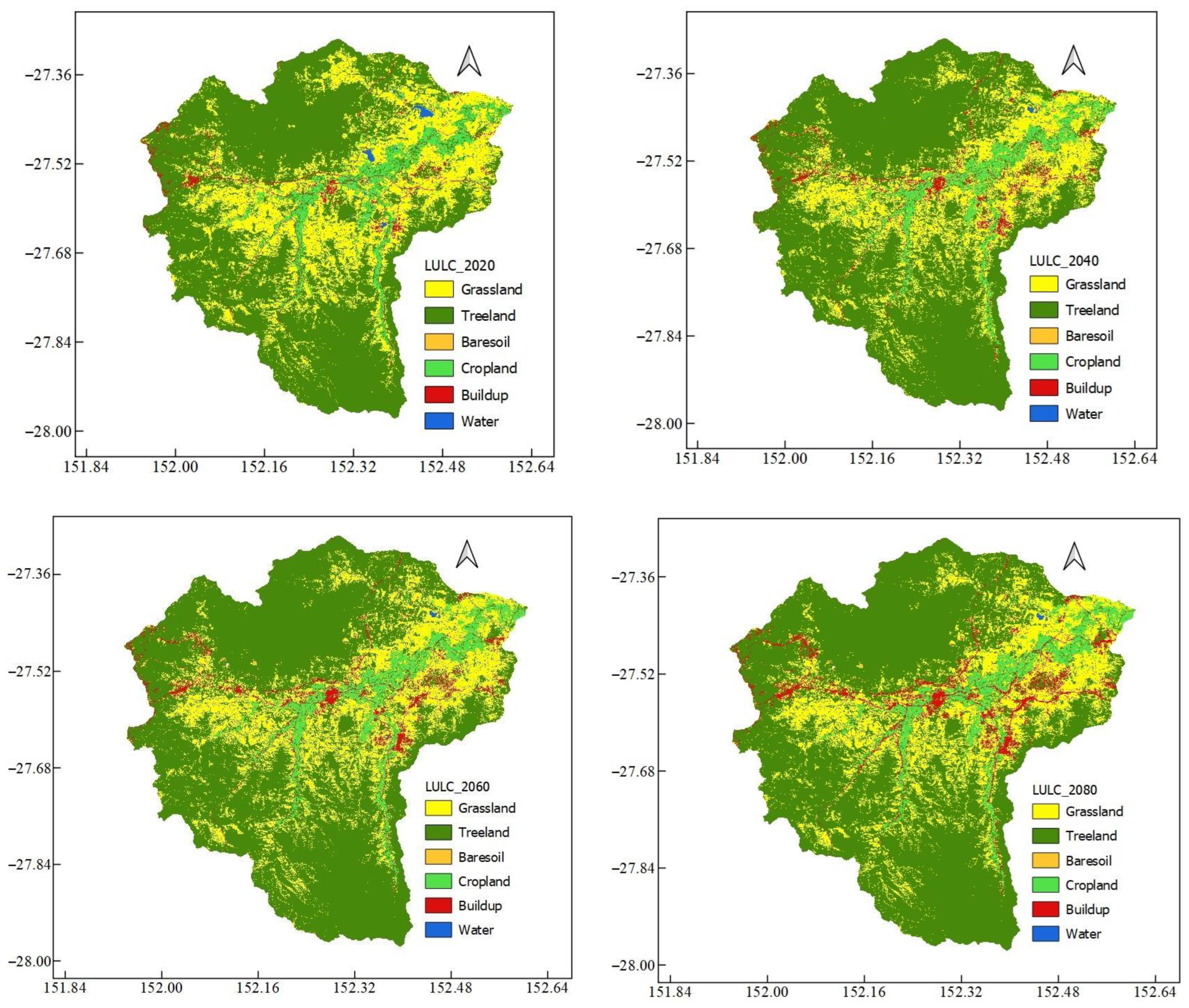
3.1. Spatiotemporal Change Analysis and Land Cover Transition Analysis

When evaluating temporal changes within a collection of land cover categories, the transition matrix is crucial. It showcases the proportions of pixels transitioning from one land cover category to another.

Table 5. Evaluation of land cover changes from 2000 to 2080.

Land Cover Classes	2000	2010	2020	2040	2060	2080
	Area in m2	Area in m2	Area in m2	Area in m2	Area in m2	Area in m2
Treeland	172,661.60	191,975.49	188,810.53	202,955.36	202,396.27	200,363.23
Grassland	102,520.44	82,108.81	81,101.62	68,640.10	68,226.88	66,685.44
Cropland	18,844.68	18,383.25	19,151.94	16,865.49	17,086.66	16,796.67
Built-up	1971.11	2963.93	5861.84	8110.32	8868.36	12,766.39
Bare Soil	224.703	338.331	568.422	112.785	108.496	98.39
Water	629.633	1099.02	1357.82	168.116	165.5	142.041

illustrates the alterations in land cover categories from 2000 to 2085. There is an indication of potential growth in built-up and tree cover areas, from 1971.11 m² in 2000 to 12,766.39 m² in 2080, and from 172,661.60 m² in 2000 to 200,363.23 m² in 2080, respectively. The findings of grassland during this period from 2000 to 2080 indicate that grassland values decreased from 102,520.44 m² in 2000 to 81,101.62 m² in 2020, followed by remarkable decrease to 68,640.10 m² in 2060 and by 66,685.44 m² in 2080.

As illustrated in Figure 4 and Table 5, there has been a consistent rise in built-up areas, starting at 1971.11 m² in 2010 and increasing to 5861.84 m² by 2020. Table 5 also shows a fourfold increase to 8868.36 m² in 2060 and sixfold increase to 12,766.39 m² in 2080. Evaluating the accuracy of classification methods is vital for understanding their reliability [44]. As shown in

Table 6. Accuracy assessment of landcover classification and projection using statistical indicators including Kappa coefficient, User’s Accuracy (UA), Producer’s Accuracy (PA), and Overall Accuracy (OA).

Year	Classification Method	Assessment Index	Landcover Classes
			TreeLand	GrassLand	CropLand	Built-Up	BareSoil	Water
2000	SVM	UA	0.71	0.86	1	1	0.77	1
		PA	1	1	0.72	0.75	1	1
		Kappa	0.85
		OA	0.88
	RF	UA	0.77	0.75	1	1	0.55	1
		PA	1	1	0.8	0.45	1	1
		Kappa	0.8
		OA	0.84
2010	SVM	UA	0.84	0.83	1	1	0.7	1
		PA	1	1	0.87	0.83	0.7	1
		Kappa	0.89
		OA	0.91
	RF	UA	0.69	0.88	1	0.85	0.47	1
		PA	1	0.88	0.8	0.58	0.7	1
		Kappa	0.79
		OA	0.82
2020	SVM	UA	0.64	0.78	0.88	1	1	1
		PA	1	0.72	0.8	1	0.7	0.71
		Kappa	0.8
		OA	0.84
	RF	UA	0.71	0.77	0.94	0.83	1	1
		PA	1	0.68	0.8	1	0.7	0.76
		Kappa	0.8
		OA	0.84
Projected 2020 based on 2000–2010	SVM	UA	0.87	0.52	0.86	0.25	0.97	0.98
		PA	0.41	0.38	0.39	0.9	0.07	0.68
		Kappa	0.37
		OA	0.47
	RF	UA	0.68	0.48	0.75	0.86	0.86	0.934
		PA	0.89	0.85	0.62	0.51	0.51	0.84
		Kappa	0.65
		OA	0.71

, the results reveal that SVM has a slightly higher accuracy in the image classification. According to Table 6, the classes of treeland, grassland, and water were classified with a higher accuracy, while the accuracy for built-up and bare soil was slightly lower. The results clearly indicate that RF outperformed SVM in the projection of landcover for the year 2020, yielding 0.71 (OA) and 0.65 (Kappa), which are 23% and 28% higher than those of the SVM model, respectively (Table 6). These results are demonstrated by [71], where RF performs better than SVM. However, for the classification, SVM, in the majority of instances, outperformed RF; for example, for the year 2000, it yielded 0.88 (OA) and 0.85 (Kappa), which are 4% and 5% higher than those of the RF model, respectively.

The classification SVM method in the year 2000 had an Overall Accuracy (OA) of 88%, Kappa of 85%, followed by User’s Accuracy (UA) of 100% for cropland and built-up areas, followed by 86% for grassland. It also had a Producer’s Accuracy (PA) of 75% for built-up areas and 72% for cropland. The Kappa and OA for the RF method were 80% and 84%, respectively. The UA results for cropland and built-up areas were similar to the SVM method. Grassland and bare soil in terms of UA decreased to 75% and 55%.

The SVM and RF for the year 2010 showed 89% (Kappa) and 91% (OA), and 79% (Kappa) and 82% (OA). In terms of individual class accuracy, the UA indicated 84% (SVM method) and 69% (RF method) for treeland, while the PA was 100% for both methods. The results of the OA (0.84) and Kappa (0.8) were the same in both the SVM and RF models for the year 2020. However, for the individual classification, which contains two classes (grassland and built-up), the SVM model generated a better user’s accuracy and producer’s accuracy. As can be observed from Table 6, RF outperformed SVM in the projection of landcover for the year 2020, and classified all six classes with a better accuracy than the SVM in terms of the Kappa, OA, and PA. The model incorporates spatial elements like distance from major roads, DEM, and population density to generate a map illustrating changes in land cover, revealing the evolving patterns within the Lockyer catchment (Figure 5).

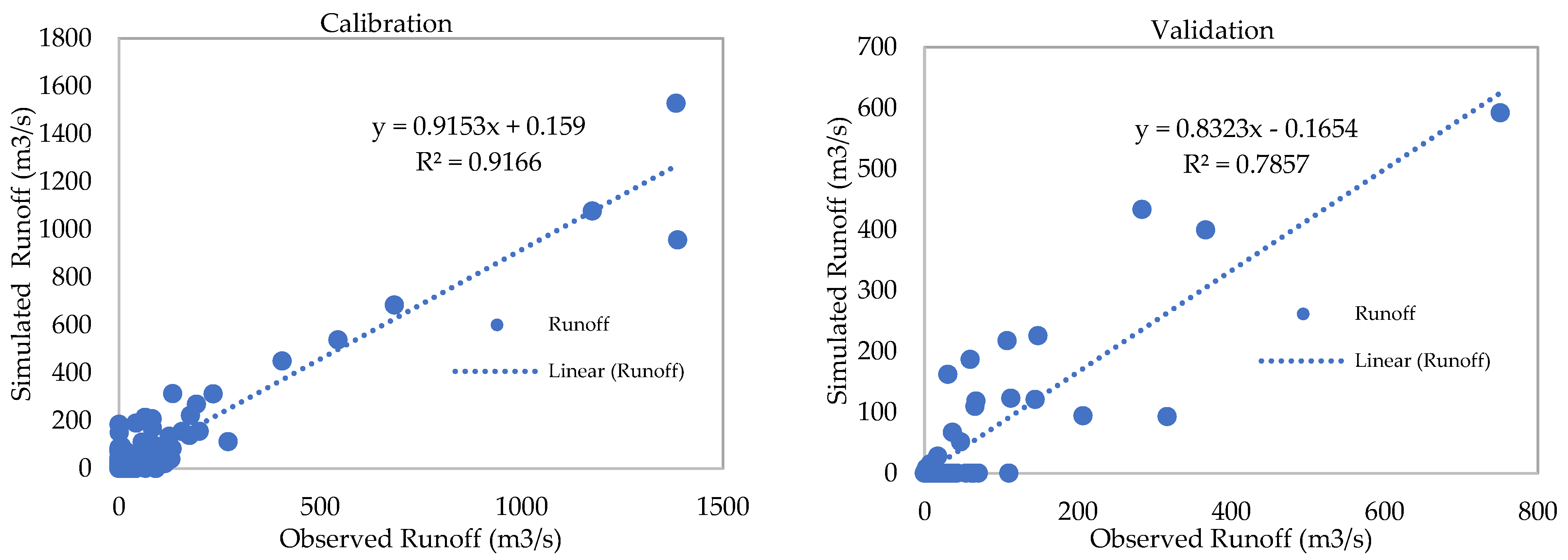
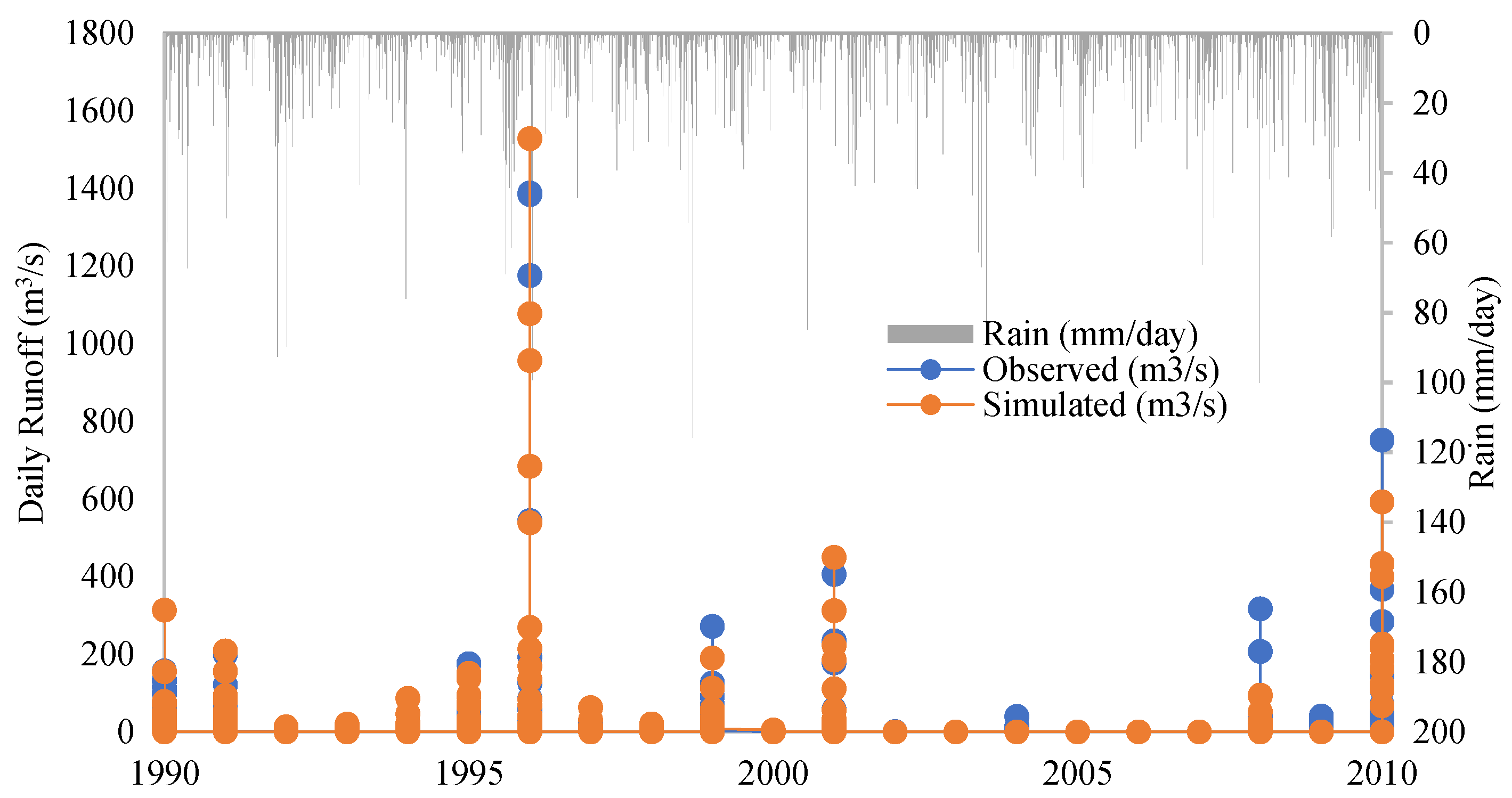
3.2. The Performance of Hydrological Model

A comparison between the simulated and observed discharge is used to assess the results of the calibration and validation for the periods of 1990–2002 and 2003–2010, respectively (Figure 6 and Figure 7). The eight calibrated parameters are presented in Table 3. The model’s output data were calibrated and validated using the daily streamflow records from the 143210B Lockyer Creek at Rifle Range Road station as the outlet. As illustrated in Figure 2, the Lockyer catchment contains eighteen rainfall-gauging stations. The model utilised inputs consisting of the area’s average weighted daily evapotranspiration and rainfall from these 18 gauging stations, along with daily records of discharge from the Rifle Range Road station. The calibration and validation of the hydrologic model were carried out for the periods of 1990–2002 and 2003–2010, respectively. Streamflow data were utilised, allocating 60% for calibration and 40% for validation purposes. According to the results of

Table 7. Daily operational data for the AWBM model during the calibration and validation periods.

	Calibration (1990–2002)	Validation (2003–2010)
R2	0.92	0.786
Nash	0.89	0.753
RMSE	0.005	0.409
BIAS	0.0004	1.206

and Figure 6, the findings indicate the model’s effective performance and its reliable accuracy in estimating runoff.

Over the calibration, R² and Nash were very good, at 92% and 89%, respectively, for the period of 1990–2002. Moreover, PBAIS indicated that the AWBM model performance over the validation period was 1.206 m³/s (Table 7). Moreover, 78%, and 75% were the calculated R² and Nash, respectively, over the validation period. According to Figure 6, there is a good match between the observed and simulated daily discharge in the Lockyer Valley catchment. Figure 6 indicates the model’s generally satisfactory performance in simulating flow patterns, and although it slightly underestimates some peak flow instances, it effectively aligns the overall patterns of storm events between the simulations and observed records. Moreover, the accurate simulation of low-flow circumstances further indicates the reliability and competence of the AWBM model in predicting discharge. Ensemble projections depict the long-term average daily inflow at the Rifle Range Road hydrometric station for near and far future periods (2020 to 2086) under the RCP 4.5 and RCP 8.5 scenarios.

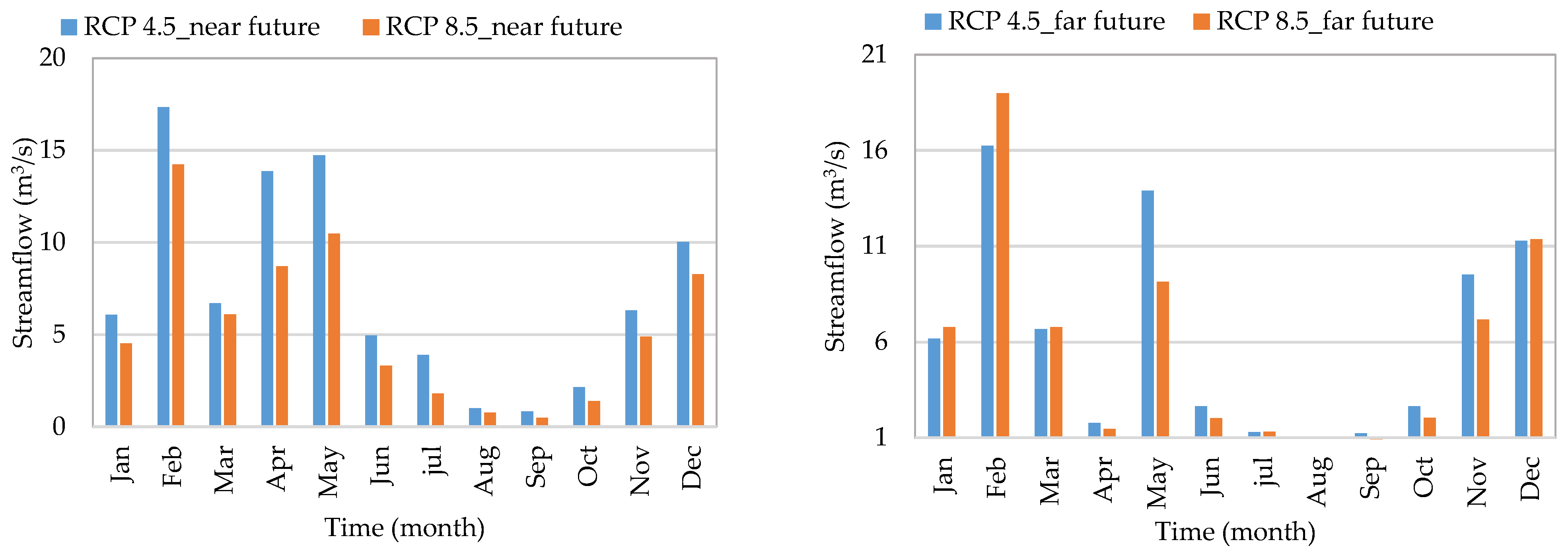
3.3. Changes in Projected Streamflow under Climate Change Scenarios

This study assessed changes in runoff factors using two climate change scenarios (RCP 4.5 and RCP 8.5) based on the combined average of eight GCMs. According to Figure 8, a decline in runoff of the ensemble of climate models was generally noticed in the far future (2066–2085) compared to the near future (2020–2065) for almost all months. In February, there was a greater variability in streamflow alterations for both RCP 4.5 and RCP 8.5, suggesting increased uncertainty in the predictions for the two future periods, as indicated by [62]. It can be concluded that the decline in streamflow will likely slow down in the far future compared to the near future, particularly between June and September.

Runoff was projected to decline in January and February by 16% in the near future and 18% in the far future. Figure 8 illustrates that the significant increase in projected runoff in February is mostly caused by the increase in projected rainfall. Also, the RCP 8.5 scenario consistently showed lower projected streamflow compared to RCP 4.5 throughout each month. February displayed the greatest span of long-term average daily streamflow from 17.35 m³/s (RC P4.5) to 14.24 m³/s (RCP 8.5) in the near future and from 16.25 m³/s (RCP 4.5) to 18.99 m³/s (RCP 8.5) in the far future. This was followed by August, which had the lowest distinction from 1 m³/s (RCP 4.5) to 0.77 m³/s (RCP 8.5) in the near future and from 0.94 m³/s (RCP 4.5) to 0.95 m³/s (RCP 8.5) in the far future. It was also evident that, in comparison to the other months, November, December, January, February, and March are expected to receive relatively high long-term streamflow levels in both future periods. In conclusion, a further increase in greenhouse gas emissions will notably intensify the impact of increasing the amount of runoff [72] in some months in the future in the Lockyer catchment.

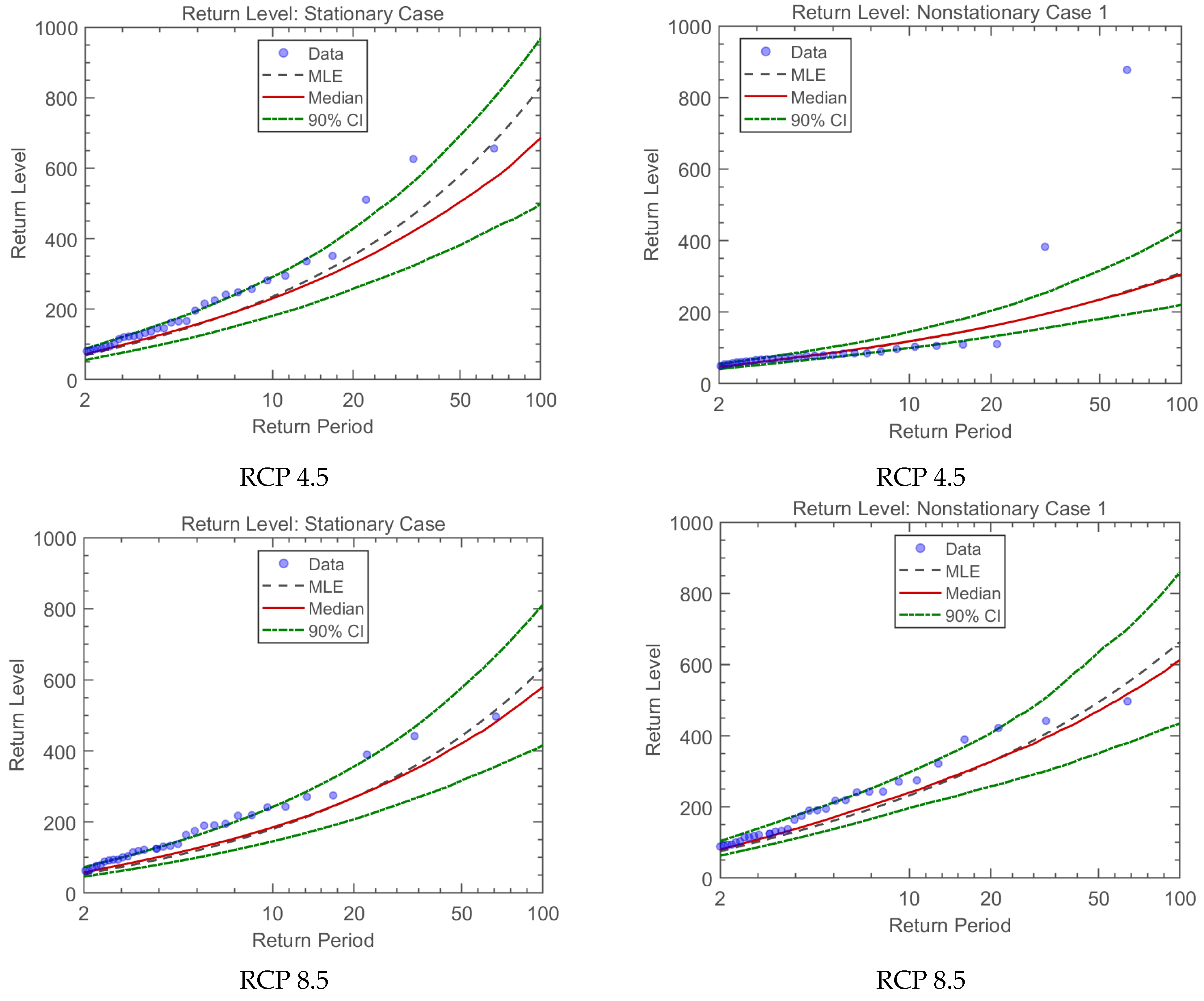
3.4. The Impacts of Climate Change on Extreme Runoff under Stationary and Non-Stationary Conditions

This research aims to investigate the non-stationary conditions of flood projected from the averaged ensemble of eight GCMs under the two scenarios RCP 4.5 and RCP 8.5 during future periods for 66 years. Figure 9 and

Table 8. The maxim runoff (m³/s) in different return periods in the Lockyer Catchment.

Return Period	Future (RCP 4.5) (m3/s)		Differences %	Future (RCP 8.5) (m3/s)		Differences %
	Stationary	Non-Stationary		Stationary	Non-Stationary
10	230.42	269.37	16.90	185.05	228.50	12.67
25	358.94	396.47	10.45	301.60	347.4	15.18
50	499.86	540.48	8.12	424.85	455.67	7.25
75	574.48	635.67	10.56	505.77	548.49	8.44
100	686	726.43	5.89	580.75	608.52	4.78

illustrate the return levels of maximum instantaneous flood for the study catchment. The ProNEVA software created streamflow return levels based on return periods spanning from 10 to 100 years under two non-stationary and stationary conditions. The greatest instantaneous flood under both stationary and non-stationary assumptions for the 2020–2086 future timeframe is illustrated in Figure 9 for 100 years beyond observations using the medians under the two RCP 4.5 and RCP 8.5 scenarios for various return durations.

For both the RCP 4.5 and RCP 8.5 scenarios, Table 8 shows the maximum flood for varying return durations, assuming two assumptions in the future periods (Table 8 is a summary of Figure 9). The 100 year return period and 25 year return period maximum floods in the Lockyer catchment for RCP4.5 vary from 686 m³/s (stationary) to 726.43 m³/s (non-stationary) and from 358.94 m³/s to 396.47 m³/s (non-stationary). For the design flood for a 100 year period, the change between the stationary and non-stationary assumption was quite similar, at 5.89% for RCP 4.5 in comparison to 4.78% for RCP 8.5, whereas in the 10 year return period, the difference between the stationary and non-stationary assumption shows more variability, from 230.42 m³/s to 269.37 m³/s (RCP 4.5) compared with 185.05 m³/s to 228.50 m³/s (RCP 8.5). According to Table 8 and Figure 9, the highest floods in the stationary assumption generally appear smaller compared to the maximum sudden floods in the non-stationary assumption across both scenarios.

As the return period extends, it shows a decline most of the time. Additionally, the findings indicate the contrast between the peak sudden flood, assuming stationary versus non-stationary conditions in both scenarios for the period from 2020 to 2086. The greatest difference for RCP 8.5 is 15.18% (25 year return period) and for RCP 4.5 is 16.90% (10 year return period). The difference between the non-stationary and stationary assumption in RCP 4.5 is greater than that in RCP 8.5 in all return periods. The peak flood return levels in low return level periods were indicated to have noticeable variations compared to high return periods.

4. Discussion

Simple regression models are examined by scholars for modelling changes in the mean, variance, and skewness and combining such non-stationary moments with various pdfs to update design events, given historical research [12,73]. The increasing concern regarding climate change brought on by a rise in greenhouse gas concentrations in the environment is another factor contributing to the growing emphasis on non-stationarity [1,74]. So, in this research, ProNEVA offers parameter estimation, uncertainty quantification, and a comprehensive assessment that allows for a non-stationary analysis using user-defined variables, which can be time or a physical variable. The advantage of performing a stationary analysis with physically related covariates lies in the possibility of imposing physical constraints on a statistical model [28].

In this research, both the non-stationary and stationary conditions for maximum instantaneous flood were investigated. The purpose of this study was to look at the non-stationary possibilities of the Lockyer catchment’s maximum instantaneous flood in the future. To achieve this aim, we developed a multi-framework by integrating a hydrological model, SVM and RF classifications in the GEE platform, an ensemble of GCMs under two RCPs, and the ProNEVA model, for the aim of evaluating the impacts of climate change on floods, streamflow, and water supply in both stationary and non-stationary conditions. SVM and RF classifications in the GEE platform were used to estimate the projected land cover changes in the future period and, by assuming a linear relationship between the location parameter and time, the ProNEVA model was applied to assess the magnitude and frequency of extreme floods utilising the GEV distribution.

According to the ARR guideline, [29] states that the GEV distribution should be applied for the purpose of designing floods and rainfalls. Earlier research on extremes [13,75,76] aligns closely with the characteristics outlined in the GEV distribution. Even with notable progress [77], there lacks an all-encompassing structure that integrates the commonly employed EVA statistical models, specifically, GEV, GP, and LP3, accounting for both stationary and non-stationary assumptions (where parameters vary with time or specific covariates) [28]. This research examines both the ProNEVA and land cover classification approaches to account for the cause-and-effect dynamics within the physical system. The model incorporates spatial factors like DEM, distance from road, and population density along with the SVM and RF classification models to produce a map illustrating land cover changes.

ProNEVA [28] incorporates the underlying physical drivers triggering extreme events, serving as a crucial instrument for quantifying the probability of extreme occurrences in a particular area or timeframe. This study investigates both ProNEVA and land cover classification to comprehensively address the cause-and-effect dynamics within the physical system. Since our focus was solely on non-stationary conditions in extreme events, using ProNEVA with a time covariant by incorporating the outputs of the ensemble of GCMs under different scenarios from the hydrological model and GEE classification approach, it is recommended that, in future studies, ProNEVA allows for the incorporation of the physical drivers as additional covariates for flood frequency analysis and modelling.

A script was coded using GEE to compute the percentage of area change per year, generating a transition matrix demonstrating the pixel shifts between different land covers. This approach was chosen due to its straightforward estimation process, which is well-suited for practical use. Enhancing the lumped conceptual hydrological model projection involves integrating various land covers by recognizing distinct land cover types and understanding how these types affect the model parameters, guided by the land cover classification map. This integration considers the influences of different land covers on evapotranspiration processes. The outcomes distinctly demonstrate that the inclusion of each land cover within the hydrological model leads to improved accuracy in the model’s results. Studies have consistently emphasised the disparity between stationary and non-stationary when incorporating the non-stationary condition [13,28,75]. Therefore, using the classification method through GEE presents an appealing option for assessing spatial and temporal aspects across regional and continental scales. The maximum instantaneous flood in the non-stationary assumption generally shows greater values compared to the maximum peak floods in the stationary assumption in both the RCP 4.5 and RCP 8.5 scenarios for different return levels. Generally, the range of uncertainty between stationary and non-stationary conditions tends to widen from 50 year to 75 year return level periods. Under the RCP 8.5 scenario, there is comparatively less variation between stationary and non-stationary conditions, whereas RCP 4.5 demonstrates a more pronounced difference. The outcomes of the trend analysis on future periods’ maximum peak flood data reveal a growing disparity in the maximum instantaneous flood between stationary and non-stationary assumptions. This suggests that the increasing difference may be a compelling reason to analyse extremes with non-stationary conditions. Moreover, exploring the variability of the scale parameter over time, both linearly and non-linearly, is possible. Analysing the impact of simultaneously incorporating non-stationarity assumptions in both scale and shape parameters on the outcomes is also a potential area of investigation for future studies.

5. Conclusions

The outputs from this study can be utilised in risk assessments and for devising adaptation strategies for state government authorities and local councils. This framework applies to diverse geographic regions, delivering vital information about extreme events such as floods necessary for risk evaluation, infrastructure design, and disaster response. Examining the non-stationary assumption in extreme flood events analysis presents a novel concern in the Lockyer catchment. Given the presence of water reservoirs, urban and rural zones, and cultivable lands in this area, forecasting the return period values for extreme floods in future periods becomes crucial, which will assist water planners, decision makers, and local communities in constructing water systems and managing resources by activating emergency response operations.

ProNEVA outcomes, when considering the physical drivers, highlight that disregarding the non-stationary condition and trends in extreme flood data leads to inaccuracies in estimating these floods across various return periods, often resulting in underestimations. This leads to flaws in the construction of hydraulic infrastructure and results in human and financial losses. Through the quantification of the likelihood of extreme events, decision makers can make well-informed decisions related to infrastructure development, resource allocation, and emergency planning. The findings of this study will assist water planners in exploring potential adaptation strategies while considering expected future alterations. It should be noted that the effectiveness of future land cover projections and hydrological simulations depends on the accuracy of the input data and assumptions made in the modelling process.

There are natural constraints that limit the accuracy of future projections, including uncertainties associated with climate projections and scenarios. The study recommends using a multi-framework approach that integrates both physical system understanding and statistical methods to gain a deeper understanding of non-stationary assumptions in extreme events at the catchment scale. The research could lead to future studies that incorporate comprehensive uncertainty analysis techniques to assess model predictions’ reliability under various climate change scenarios. Furthermore, investigating innovative techniques for capturing and integrating non-stationary trends in hydrological processes could improve model predictability and facilitate more robust decision making.

References

1. IPCC. Climate Change 2007: Synthesis Report. Contribution of Working Groups I, II and III to the Fourth Assessment Report of the Intergovernmental Panel on Climate Change; Core Writing Team, Pachauri, R.K., Reisinger, A., Eds.; Cambridge University Press: Cambridge, UK, 2007; p. 104. [Google Scholar]
2. IPCC. Climate Change 2014: Synthesis Report. Contribution of Working Groups I, II and III to the Fifth Assessment Report of the Intergovernmental Panel on Climate Change; Cambridge University Press: Cambridge, UK, 2014. [Google Scholar]
3. Wang, J.; Hu, C.; Ma, B.; Mu, X. Rapid urbanization impact on the hydrological processes in Zhengzhou, China. Water 2020, 12, 1870. [Google Scholar] [CrossRef]
4. Ding, Y.; Zhang, Y.; Song, J. Changes in Weather and Climate Extreme Events and Their Association with the Global Warming. Meteorol. Mon. 2002, 28, 3–7. [Google Scholar]
5. Wang, Q.; Xu, Y.; Wang, Y.; Zhang, Y.; Xiang, J.; Xu, Y.; Wang, J. Individual and combined impacts of future land-use and climate conditions on extreme hydrological events in a representative basin of the Yangtze River Delta, China. Atmos. Res. 2020, 236, 104805. [Google Scholar] [CrossRef]
6. Head, L.; Adams, M.; McGregor, H.V.; Toole, S. Climate change and Australia. Wiley Interdiscip. Rev. Clim. Change 2014, 5, 175–197. [Google Scholar] [CrossRef]
7. Al-Safi, H.I.J.; Sarukkalige, P.R. Assessment of future climate change impacts on hydrological behavior of Richmond River Catchment. Water Sci. Eng. 2017, 10, 197–208. [Google Scholar] [CrossRef]
8. Ramezani, M.R.; Helfer, F.; Yu, B. Individual and combined impacts of urbanization and climate change on catchment runoff in Southeast Queensland, Australia. Sci. Total Environ. 2023, 861, 160528. [Google Scholar] [CrossRef] [PubMed]
9. Lamichhane, S.; Shakya, N.M. Integrated assessment of climate change and land use change impacts on hydrology in the Kathmandu Valley watershed, Central Nepal. Water 2019, 11, 2059. [Google Scholar] [CrossRef]
10. Meaurio, M.; Zabaleta, A.; Boithias, L.; Epelde, A.M.; Sauvage, S.; Sánchez-Pérez, J.-M.; Srinivasan, R.; Antiguedad, I. Assessing the hydrological response from an ensemble of CMIP5 climate projections in the transition zone of the Atlantic region (Bay of Biscay). J. Hydrol. 2017, 548, 46–62. [Google Scholar] [CrossRef]
11. Bloschl, G.; Montanari, A. Climate change impacts—Throwing the dice? Hydrol. Process. Int. J. 2010, 24, 374–381. [Google Scholar] [CrossRef]
12. Salas, J.; Obeysekera, J.; Vogel, R. Techniques for assessing water infrastructure for nonstationary extreme events: A review. Hydrol. Sci. J. 2018, 63, 325–352. [Google Scholar] [CrossRef]
13. Pakdel, H.; Paudyal, D.R.; Chadalavada, S.; Alam, M.J.; Vazifedoust, M. A Multi-Framework of Google Earth Engine and GEV for Spatial Analysis of Extremes in Non-Stationary Condition in Southeast Queensland, Australia. ISPRS Int. J. Geo-Inf. 2023, 12, 370. [Google Scholar] [CrossRef]
14. Cheng, L.; AghaKouchak, A.; Gilleland, E.; Katz, R.W. Non-stationary extreme value analysis in a changing climate. Clim. Change 2014, 127, 353–369. [Google Scholar] [CrossRef]
15. Cooley, D. Extreme value analysis and the study of climate change. Clim. Change 2009, 97, 77–83. [Google Scholar] [CrossRef]
16. Love, C.A.; Skahill, B.E.; Russell, B.T.; Baggett, J.S.; AghaKouchak, A. An Effective Trend Surface Fitting Framework for Spatial Analysis of Extreme Events. Geophys. Res. Lett. 2022, 49, e2022GL098132. [Google Scholar] [CrossRef]
17. Salas, J.D.; Obeysekera, J. Revisiting the concepts of return period and risk for nonstationary hydrologic extreme events. J. Hydrol. Eng. 2014, 19, 554–568. [Google Scholar] [CrossRef]
18. Cooley, D. Return periods and return levels under climate change. In Extremes in a Changing Climate; AghaKouchak, A., Easterling, D., Hsu, K., Schubert, S., Sorooshian, S., Eds.; Water Science and Technology Library; Springer: Dordrecht, The Netherlands, 2013; Volume 65, pp. 97–114. [Google Scholar]
19. Burn, D.H.; Sharif, M.; Zhang, K. Detection of trends in hydrological extremes for Canadian watersheds. Hydrol. Process. 2010, 24, 1781–1790. [Google Scholar] [CrossRef]
20. Gislason, P.O.; Benediktsson, J.A.; Sveinsson, J.R. Random forests for land cover classification. Pattern Recognit. Lett. 2006, 27, 294–300. [Google Scholar] [CrossRef]
21. Gualtieri, J.A.; Cromp, R.F. Support vector machines for hyperspectral remote sensing classification. In Proceedings of the 27th AIPR Workshop: Advances in Computer-Assisted Recognition, Washington, DC, USA, 14–16 October 1998; pp. 221–232. [Google Scholar]
22. Jones, B.; Tebaldi, C.; O’Neill, B.C.; Oleson, K.; Gao, J. Avoiding population exposure to heat-related extremes: Demographic change vs climate change. Clim. Change 2018, 146, 423–437. [Google Scholar] [CrossRef]
23. Khaliq, M.N.; St-Hilaire, A.; Ouarda, T.B.; Bobée, B. Frequency analysis and temporal pattern of occurrences of southern Quebec heatwaves. Int. J. Climatol. A J. R. Meteorol. Soc. 2005, 25, 485–504. [Google Scholar] [CrossRef]
24. Rainham, D.G.; Smoyer-Tomic, K.E. The role of air pollution in the relationship between a heat stress index and human mortality in Toronto. Environ. Res. 2003, 93, 9–19. [Google Scholar] [CrossRef] [PubMed]
25. Huth, R.; Kyselý, J.; Pokorná, L. A GCM simulation of heat waves, dry spells, and their relationships to circulation. Clim. Change 2000, 46, 29–60. [Google Scholar] [CrossRef]
26. Ouarda, T.B.; Charron, C. Nonstationary temperature-duration-frequency curves. Sci. Rep. 2018, 8, 15493. [Google Scholar] [CrossRef] [PubMed]
27. Cheng, L.; AghaKouchak, A. Nonstationary precipitation intensity-duration-frequency curves for infrastructure design in a changing climate. Sci. Rep. 2014, 4, 7093. [Google Scholar] [CrossRef] [PubMed]
28. Ragno, E.; AghaKouchak, A.; Cheng, L.; Sadegh, M. A generalized framework for process-informed nonstationary extreme value analysis. Adv. Water Resour. 2019, 130, 270–282. [Google Scholar] [CrossRef]
29. Ball, J.; Babister, M.; Nathan, R.; Weinmann, P.; Weeks, W.; Retallick, M.; Testoni, I. Australian Rainfall and Runoff—A Guide to Flood Estimation; Open Publications of UTS Scholars: Ultimo, NSW, Australia, 2019. [Google Scholar]
30. Montanari, A.; Koutsoyiannis, D. Modeling and mitigating natural hazards: Stationarity is immortal! Water Resour. Res. 2014, 50, 9748–9756. [Google Scholar] [CrossRef]
31. Usman, M.; Ndehedehe, C.E.; Farah, H.; Manzanas, R. Impacts of climate change on the streamflow of a large river basin in the Australian tropics using optimally selected climate model outputs. J. Clean. Prod. 2021, 315, 128091. [Google Scholar] [CrossRef]
32. Vance, T.; Roberts, J.; Plummer, C.; Kiem, A.; Van Ommen, T. Interdecadal Pacific variability and eastern Australian megadroughts over the last millennium. Geophys. Res. Lett. 2015, 42, 129–137. [Google Scholar] [CrossRef]
33. Sarker, A.; Ross, H.; Shrestha, K.K. A common-pool resource approach for water quality management: An Australian case study. Ecol. Econ. 2008, 68, 461–471. [Google Scholar] [CrossRef]
34. Enquiry, Q.F.C. Interim Report, 1 August 2011; Queensland Floods Commission of Inquiry: Brisbane, Australia, 2011. Available online: http://www.floodcommission.qld.gov.au/publications/interim-report (accessed on 16 April 2022).
35. Van den Honert, R.C.; McAneney, J. The 2011 Brisbane floods: Causes, impacts and implications. Water 2011, 3, 1149–1173. [Google Scholar] [CrossRef]
36. Cui, T.; Raiber, M.; Pagendam, D.; Gilfedder, M.; Rassam, D. Response of groundwater level and surface-water/groundwater interaction to climate variability: Clarence-Moreton Basin, Australia. Hydrogeol. J. 2018, 26, 593–614. [Google Scholar] [CrossRef]
37. Armstrong, M.S.; Kiem, A.S.; Vance, T.R. Comparing instrumental, palaeoclimate, and projected rainfall data: Implications for water resources management and hydrological modelling. J. Hydrol. Reg. Stud. 2020, 31, 100728. [Google Scholar] [CrossRef]
38. CSIRO; BOM. Climate Change in Australia Information for Australia’s Natural Resource Management Regions: Technical Report; CSIRO and Bureau of Meteorology: Canberra, Australia, 2015. [Google Scholar]
39. Jeffrey, S.J.; Carter, J.O.; Moodie, K.B.; Beswick, A.R. Using spatial interpolation to construct a comprehensive archive of Australian climate data. Environ. Model. Softw. 2001, 16, 309–330. [Google Scholar] [CrossRef]
40. Pakdel, H.; Vazifedoust, M.; Paudyal, D.R.; Chadalavada, S.; Alam, M.J. Google Earth Engine as Multi-Sensor Open-Source Tool for Monitoring Stream Flow in the Transboundary River Basin: Doosti River Dam. ISPRS Int. J. Geo-Inf. 2022, 11, 535. [Google Scholar] [CrossRef]
41. Mission, N.S.R.T. Shuttle Radar Topography Mission (SRTM) Global. Distributed by OpenTopography. Available online: https://www.fdsn.org/networks/detail/GH/ (accessed on 15 September 2022).
42. Zanaga, D.; Van De Kerchove, R.; Daems, D.; De Keersmaecker, W.; Brockmann, C.; Kirches, G.; Wevers, J.; Cartus, O.; Santoro, M.; Fritz, S. ESA WorldCover 10 m 2021 v200. 2022. Available online: https://pure.iiasa.ac.at/18478 (accessed on 16 April 2022).
43. Cortes, C.; Vapnik, V. Support-vector networks. Mach. Learn. 1995, 20, 273–297. [Google Scholar] [CrossRef]
44. Esmaeili, P.; Vazifedoust, M.; Rahmani, M.; Pakdel, H. A simple rule-based algorithm in Google Earth Engine for operational discrimination of rice paddies in Sefidroud Irrigation Network. Arab. J. Geosci. 2023, 16, 649. [Google Scholar] [CrossRef]
45. Pal, M.; Mather, P.M. Support vector machines for classification in remote sensing. Int. J. Remote Sens. 2005, 26, 1007–1011. [Google Scholar] [CrossRef]
46. Xie, G.; Niculescu, S. Mapping and monitoring of land cover/land use (LCLU) changes in the crozon peninsula (Brittany, France) from 2007 to 2018 by machine learning algorithms (support vector machine, random forest, and convolutional neural network) and by post-classification comparison (PCC). Remote Sens. 2021, 13, 3899. [Google Scholar] [CrossRef]
47. Briem, G.J.; Benediktsson, J.A.; Sveinsson, J.R. Multiple classifiers applied to multisource remote sensing data. IEEE Trans. Geosci. Remote Sens. 2002, 40, 2291–2299. [Google Scholar] [CrossRef]
48. Iqbal, M.S.; Dahri, Z.H.; Querner, E.P.; Khan, A.; Hofstra, N. Impact of climate change on flood frequency and intensity in the Kabul River Basin. Geosciences 2018, 8, 114. [Google Scholar] [CrossRef]
49. Zhou, Q.; Leng, G.; Huang, M. Impacts of future climate change on urban flood volumes in Hohhot in northern China: Benefits of climate change mitigation and adaptations. Hydrol. Earth Syst. Sci. 2018, 22, 305–316. [Google Scholar] [CrossRef]
50. Cui, T.; Yang, T.; Xu, C.-Y.; Shao, Q.; Wang, X.; Li, Z. Assessment of the impact of climate change on flow regime at multiple temporal scales and potential ecological implications in an alpine river. Stoch. Environ. Res. Risk Assess. 2018, 32, 1849–1866. [Google Scholar] [CrossRef]
51. Melsen, L.A.; Addor, N.; Mizukami, N.; Newman, A.J.; Torfs, P.J.; Clark, M.P.; Uijlenhoet, R.; Teuling, A.J. Mapping (dis) agreement in hydrologic projections. Hydrol. Earth Syst. Sci. 2018, 22, 1775–1791. [Google Scholar] [CrossRef]
52. Boughton, W. A hydrograph-based model for estimating the water yield of ungauged catchments. In Proceedings of the Hydrology and Water Resources Symposium, Newcastle, IEAust, Newcastle, Australia, 30 June–2 July 1993. [Google Scholar]
53. Boughton, W. The Australian water balance model. Environ. Model. Softw. 2004, 19, 943–956. [Google Scholar] [CrossRef]
54. Boughton, W.C. An Australian water balance model for semiarid watersheds. J. Soil Water Conserv. 1995, 50, 454–457. [Google Scholar]
55. Boughton, W. Calibrations of a daily rainfall-runoff model with poor quality data. Environ. Model. Softw. 2006, 21, 1114–1128. [Google Scholar] [CrossRef]
56. Boughton, W. Effect of data length on rainfall–runoff modelling. Environ. Model. Softw. 2007, 22, 406–413. [Google Scholar] [CrossRef]
57. Yu, B.; Zhu, Z. A comparative assessment of AWBM and SimHyd for forested watersheds. Hydrol. Sci. J. 2015, 60, 1200–1212. [Google Scholar] [CrossRef]
58. Jahandideh-Tehrani, M.; Zhang, H.; Helfer, F.; Yu, Y. Review of climate change impacts on predicted river streamflow in tropical rivers. Environ. Monit. Assess. 2019, 191, 752. [Google Scholar] [CrossRef] [PubMed]
59. Petheram, C.; Rustomji, P.; McVicar, T.R.; Cai, W.; Chiew, F.H.; Vleeshouwer, J.; Van Niel, T.G.; Li, L.; Cresswell, R.G.; Donohue, R.J. Estimating the impact of projected climate change on runoff across the tropical savannas and semiarid rangelands of northern Australia. J. Hydrometeorol. 2012, 13, 483–503. [Google Scholar] [CrossRef]
60. Podger, G. Rainfall Runoff Library User Guide; Cooperative Research Centre for Catchment Hydrology: Clayton, Australia, 2004. [Google Scholar]
61. Esmaeili-Gisavandani, H.; Lotfirad, M.; Sofla, M.S.D.; Ashrafzadeh, A. Improving the performance of rainfall-runoff models using the gene expression programming approach. J. Water Clim. Change 2021, 12, 3308–3329. [Google Scholar] [CrossRef]
62. Tehrani, M.J.; Helfer, F.; Jenkins, G. Impacts of climate change and sea level rise on catchment management: A multi-model ensemble analysis of the Nerang River catchment, Australia. Sci. Total Environ. 2021, 777, 146223. [Google Scholar] [CrossRef]
63. Pakdel, H.; Vazifedoust, M.; Marofi, S.; Tizro, A.T. Simulation of river discharge in ungauged catchments by forcing GLDAS products to a hydrological model (a case study: Polroud basin, Iran). Water Supply 2020, 20, 277–286. [Google Scholar] [CrossRef]
64. Eccles, R.; Zhang, H.; Hamilton, D.; Trancoso, R.; Syktus, J. Impacts of climate change on streamflow and floodplain inundation in a coastal subtropical catchment. Adv. Water Resour. 2021, 147, 103825. [Google Scholar] [CrossRef]
65. Kirono, D.G.; Round, V.; Heady, C.; Chiew, F.H.; Osbrough, S. Drought projections for Australia: Updated results and analysis of model simulations. Weather Clim. Extrem. 2020, 30, 100280. [Google Scholar] [CrossRef]
66. Alexander, L.V.; Arblaster, J.M. Historical and projected trends in temperature and precipitation extremes in Australia in observations and CMIP5. Weather Clim. Extrem. 2017, 15, 34–56. [Google Scholar] [CrossRef]
67. Durocher, M.; Burn, D.H.; Ashkar, F. Comparison of estimation methods for a nonstationary Index-Flood Model in flood frequency analysis using peaks over threshold. Water Resour. Res. 2019, 55, 9398–9416. [Google Scholar] [CrossRef]
68. Moisello, U. On the use of partial probability weighted moments in the analysis of hydrological extremes. Hydrol. Process. Int. J. 2007, 21, 1265–1279. [Google Scholar] [CrossRef]
69. Coles, S.; Bawa, J.; Trenner, L.; Dorazio, P. An Introduction to Statistical Modeling of Extreme Values; Springer: London, UK, 2001; Volume 208. [Google Scholar]
70. Morrison, J.E.; Smith, J.A. Stochastic modeling of flood peaks using the generalised extreme value distribution. Water Resour. Res. 2002, 38, 41-1–41-12. [Google Scholar] [CrossRef]
71. Adugna, T.; Xu, W.; Fan, J. Comparison of random forest and support vector machine classifiers for regional land cover mapping using coarse resolution FY-3C images. Remote Sens. 2022, 14, 574. [Google Scholar] [CrossRef]
72. Sadeghi Loyeh, N.; Massah Bavani, A. Daily maximum runoff frequency analysis under non-stationary conditions due to climate change in the future period: Case study Ghareh Sou Basin. J. Water Clim. Change 2021, 12, 1910–1929. [Google Scholar] [CrossRef]
73. Obeysekera, J.; Salas, J.D. Quantifying the uncertainty of design floods under nonstationary conditions. J. Hydrol. Eng. 2014, 19, 1438–1446. [Google Scholar] [CrossRef]
74. IPCC. Summary for Policymakers. In Climate Change 2021: The Physical Science Basis. Contribution of Working Group I to the Sixth Assessment Report of the Intergovernmental Panel on Climate Change; Masson-Delmotte, V., Zhai, P., Pirani, A., Connors, S.L., Péan, C., Berger, S., Caud, N., Chen, Y., Goldfarb, L., Gomis, M.I., et al., Eds.; IPCC: Geneva, Switzerland, 2021; In Press. [Google Scholar]
75. Lima, C.H.; Lall, U.; Troy, T.J.; Devineni, N. A climate informed model for nonstationary flood risk prediction: Application to Negro River at Manaus, Amazonia. J. Hydrol. 2015, 522, 594–602. [Google Scholar] [CrossRef]
76. Gilleland, E.; Katz, R.W. New software to analyze how extremes change over time. Eos Trans. Am. Geophys. Union 2011, 92, 13–14. [Google Scholar] [CrossRef]
77. Sarhadi, A.; Soulis, E.D. Time-varying extreme rainfall intensity-duration-frequency curves in a changing climate. Geophys. Res. Lett. 2017, 44, 2454–2463. [Google Scholar] [CrossRef]
Figure 1. Flowchart of GCMs projections, hydrological model, GEE, and GEV model to estimate streamflow extremes.
Ijgi 13 00123 g001
Figure 2. The study’s area geographical position in Australia (Left) and hydro-meteorological stations are taken into consideration throughout the catchment (Right).
Ijgi 13 00123 g002
Figure 3. Land cover changes workflow chart (a) and spatial distribution of both training and validation polygons (b).
Ijgi 13 00123 g003
Figure 4. Land cover changes from 2000 to 2080 in the Lockyer catchment.
Ijgi 13 00123 g004aIjgi 13 00123 g004b
Figure 5. Spatial variables applied to the landcover changes projection in the Lockyer catchment.
Ijgi 13 00123 g005
Figure 6. Scatter plot of observed and simulated daily runoff at the Lockyer valley over the calibration (1990–2002) and validation periods (2003–2010).
Ijgi 13 00123 g006
Figure 7. Observed and simulated daily runoff at the Lockyer Valley over the calibration (1990–2002) and validation periods (2003–2010).
Ijgi 13 00123 g007
Figure 8. Ensemble projections of long-term average daily inflow at Lockyer Creek at Rifle Range Road station for near future (2020–2065) and far future (2066–2085) periods under RCP 4.5 and RCP 8.5.
Ijgi 13 00123 g008
Figure 9. NEVA’s non-stationary GEV framework output, standard return levels with the likelihood of design exceedance for flood for future periods (2020–2086) under stationary and non-stationary assumption. (Figure generated using MATLAB R2020b).
Ijgi 13 00123 g009