
Exploring the Influence of Terrain Blockage on Spatiotemporal Variations in Land Surface Temperature from the Perspective of Heat Energy Redistribution

Abstract
:1. Introduction
2. Materials
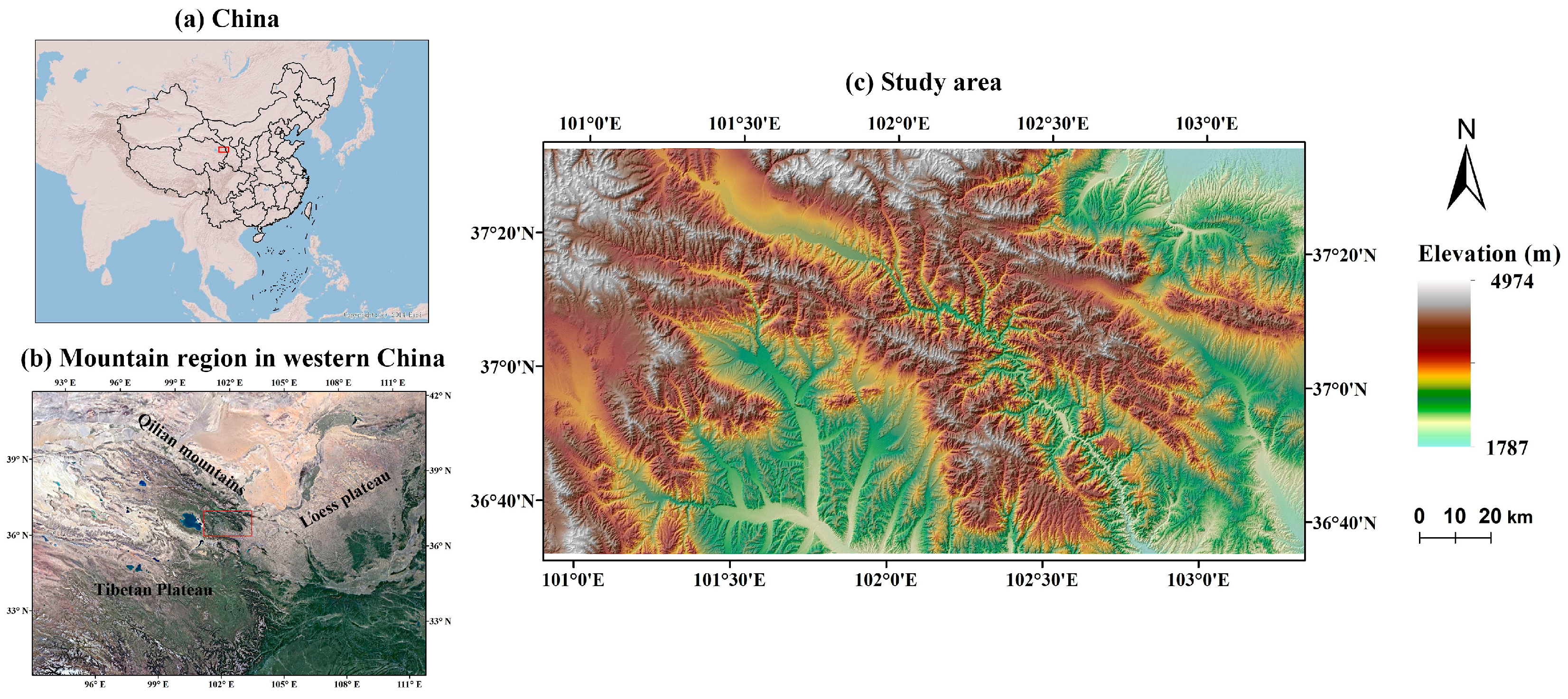
2.1. Study Area
2.2. Data
2.2.1. Digital Elevation Model
2.2.2. LST Data
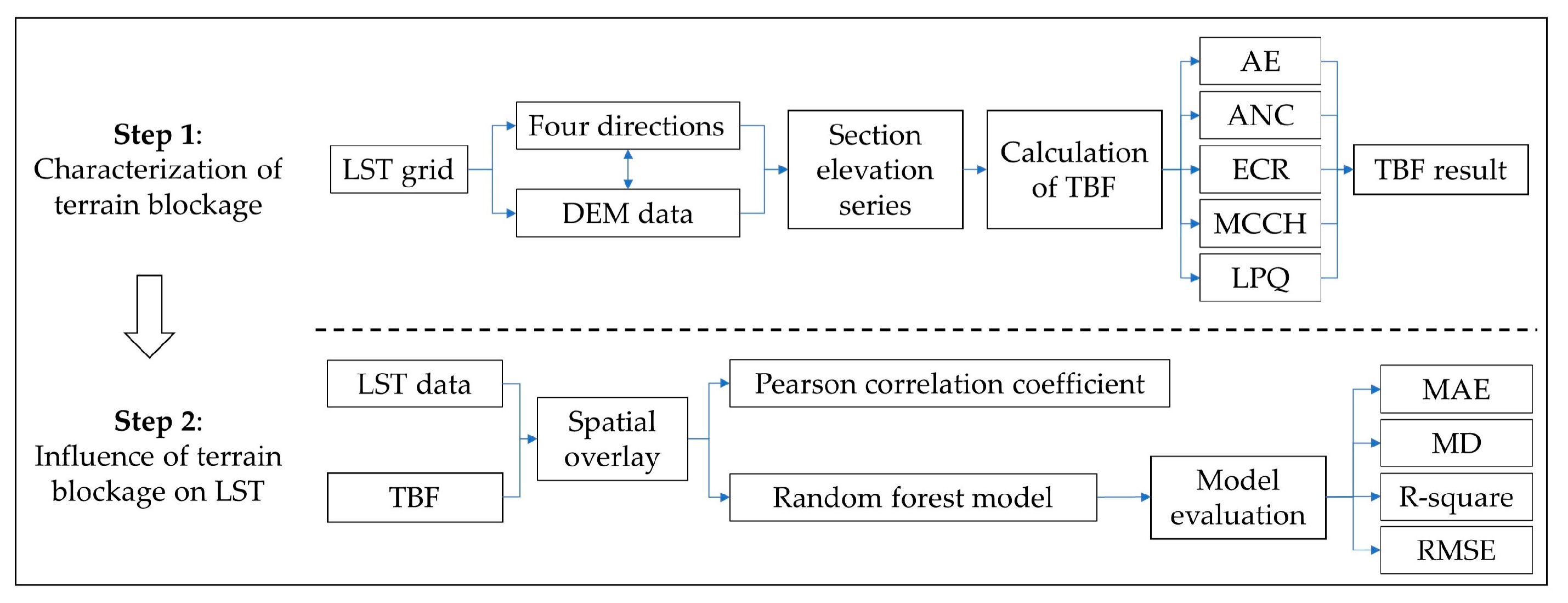
3. Methods
3.1. Characterization of Terrain Blockage in the Process of Heat Energy Redistribution
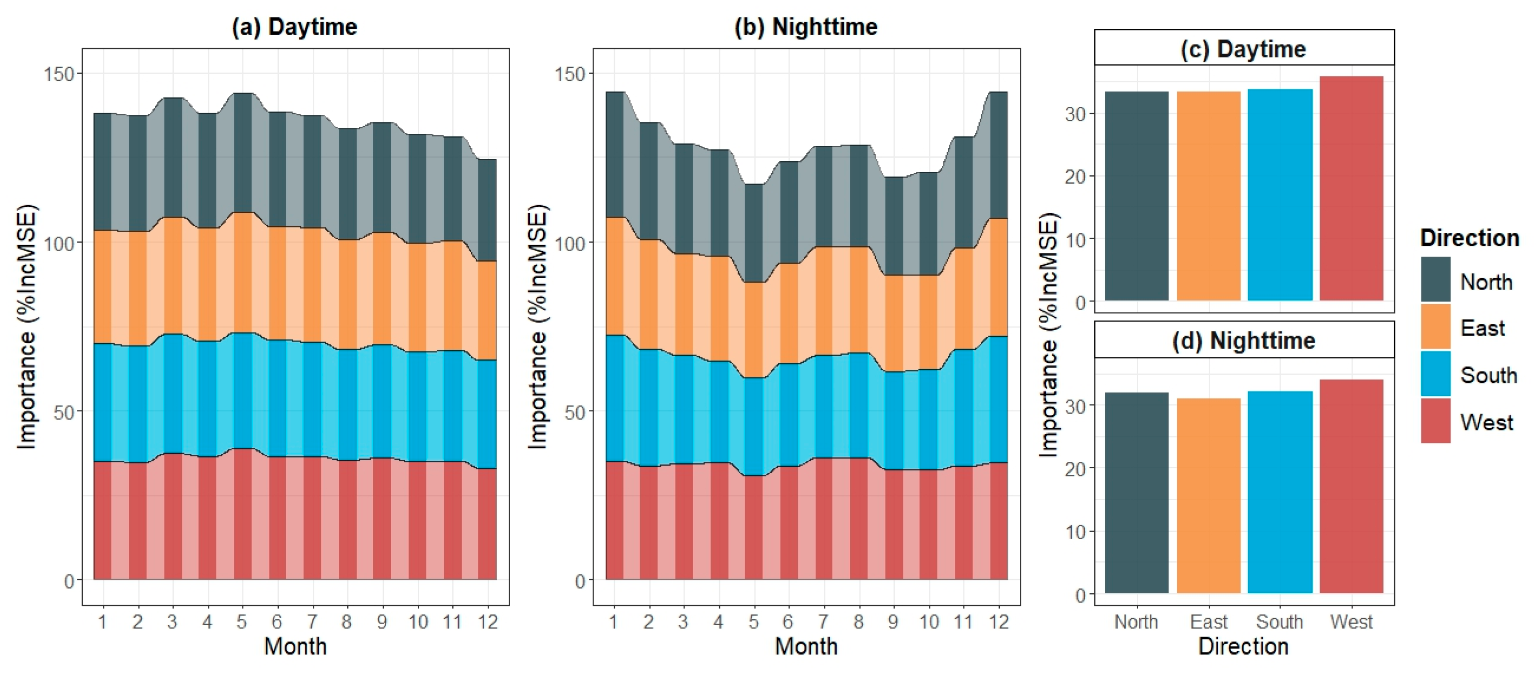
3.1.1. Extracting Section Elevation Series in Major Directions
3.1.2. Generation of TBFs Using Serial Values of Section Elevation
3.2. Simulating the Relationship between TBFs and LST Using a Random Forest Model
3.3. Statistical Indices for Evaluating Model Results
4. Results
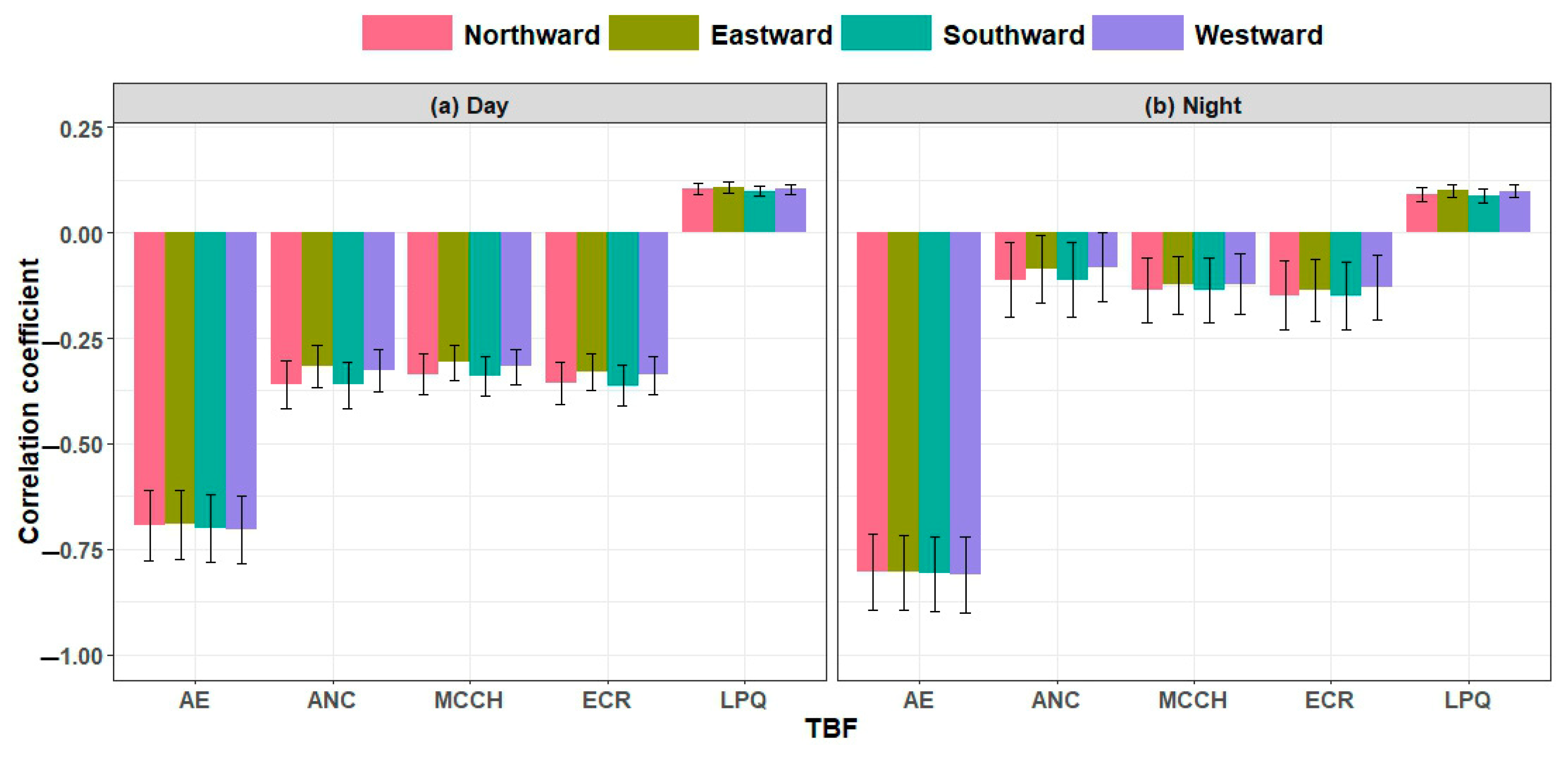
4.1. Correlation Coefficient Analysis for TBF and LST
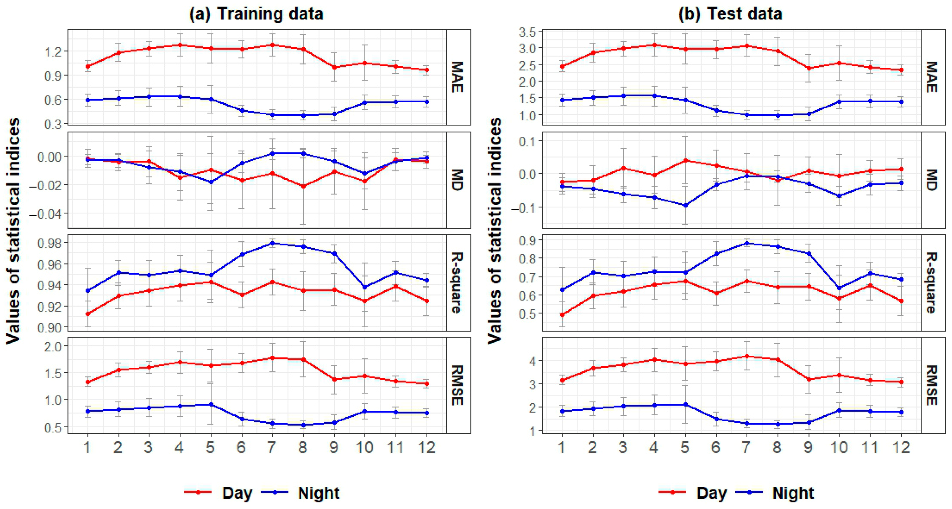
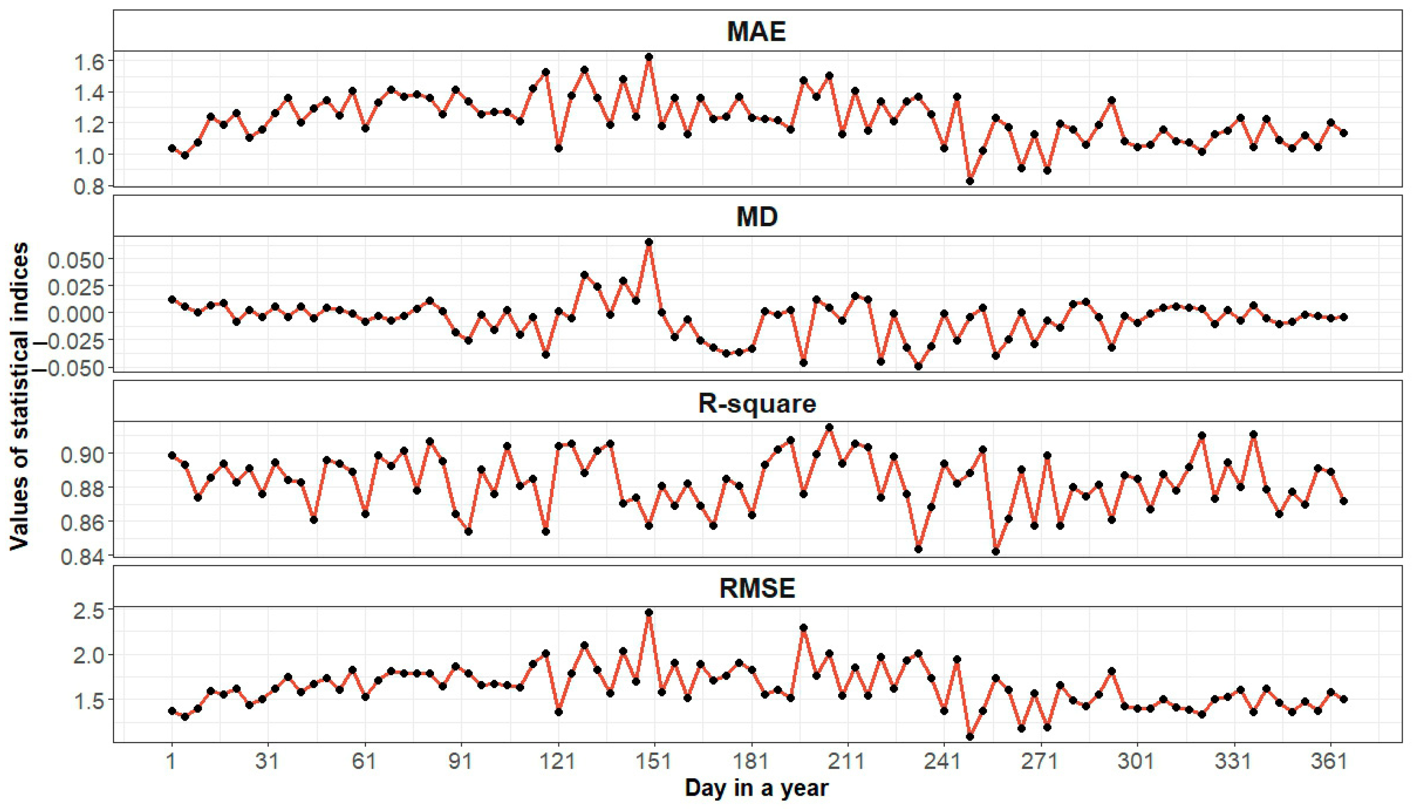
4.2. Temporal Patterns for LST Simulated Using TBF and Their Accuracy
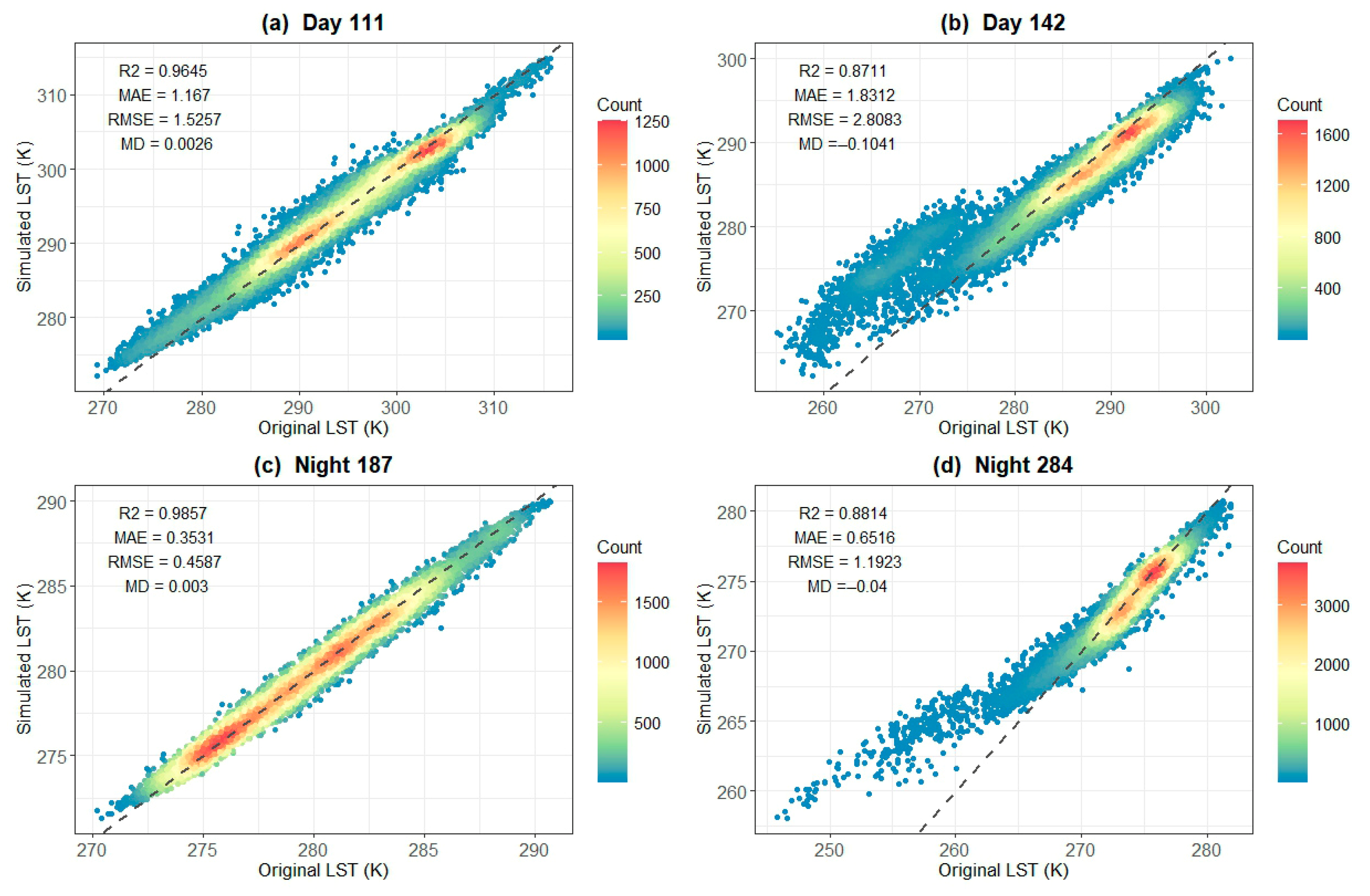
4.3. Comparison of Spatial Distribution between Original and Simulated LST
5. Discussion
5.1. Comparing First Distribution with Redistribution of Heat Energy in Mountain Regions
5.2. Directions in Characterizing Terrain Blockage Caused by Raised Mountains
5.3. Predictive Power of Terrain Blockage for Other Properties of Thermal Environment
5.4. Limitations and Usefulness
6. Conclusions
Author Contributions
Funding
Data Availability Statement
Acknowledgments
Conflicts of Interest
References
- Fuldauer, L.I.; Thacker, S.; Haggis, R.A.; Fuso-Nerini, F.; Nicholls, R.J.; Hall, J.W. Targeting climate adaptation to safeguard and advance the Sustainable Development Goals. Nat. Commun. 2022, 13, 15. [Google Scholar] [CrossRef] [PubMed]
- Liu, J.L.; Tang, H.Y.; Yan, F.Q.; Liu, S.W.; Tang, X.G.; Ding, Z.; Yu, P.J. Future variation of land surface temperature in the Yangtze River Basin based on CMIP6 model. Int. J. Digit. Earth 2023, 16, 2776–2796. [Google Scholar] [CrossRef]
- Massaro, E.; Schifanella, R.; Piccardo, M.; Caporaso, L.; Taubenböck, H.; Cescatti, A.; Duveiller, G. Spatially-optimized urban greening for reduction of population exposure to land surface temperature extremes. Nat. Commun. 2023, 14, 10. [Google Scholar] [CrossRef] [PubMed]
- Xie, X.Y.; Tian, J.; Wu, C.L.; Li, A.N.; Jin, H.A.; Bian, J.H.; Zhang, Z.J.; Nan, X.; Jin, Y. Long-term topographic effect on remotely sensed vegetation index-based gross primary productivity (GPP) estimation at the watershed scale. Int. J. Appl. Earth Obs. Geoinf. 2022, 108, 12. [Google Scholar] [CrossRef]
- Mushore, T.D.; Mutanga, O.; Odindi, J. Understanding Growth-Induced Trends in Local Climate Zones, Land Surface Temperature, and Extreme Temperature Events in a Rapidly Growing City: A Case of Bulawayo Metropolitan City in Zimbabwe. Front. Environ. Sci. 2022, 10, 14. [Google Scholar] [CrossRef]
- Zhao, W.; Duan, S.B.; Li, A.N.; Yin, G.F. A practical method for reducing terrain effect on land surface temperature using random forest regression. Remote Sens. Environ. 2019, 221, 635–649. [Google Scholar] [CrossRef]
- Zhu, J.; Ren, H.; Ye, X.; Teng, Y.; Zeng, H.; Liu, Y.; Fan, W. PKULAST-An Extendable Model for Land Surface Temperature Retrieval From Thermal Infrared Remote Sensing Data. IEEE J. Sel. Top. Appl. Earth Obs. Remote Sens. 2022, 15, 9278–9292. [Google Scholar] [CrossRef]
- Zhao, H.; Ren, H.; Fu, G. An Analytic Solution Method for Retrieving Land Surface Temperature from Remotely Sensed Thermal Infrared Imagery. J. Indian Soc. Remote Sens. 2015, 43, 279–286. [Google Scholar] [CrossRef]
- Duan, S.-B.; Li, Z.-L.; Leng, P. A framework for the retrieval of all-weather land surface temperature at a high spatial resolution from polar-orbiting thermal infrared and passive microwave data. Remote Sens. Environ. 2017, 195, 107–117. [Google Scholar] [CrossRef]
- Duan, S.-B.; Han, X.-J.; Huang, C.; Li, Z.-L.; Wu, H.; Qian, Y.; Gao, M.; Leng, P. Land Surface Temperature Retrieval from Passive Microwave Satellite Observations: State-of-the-Art and Future Directions. Remote Sens. 2020, 12, 2573. [Google Scholar] [CrossRef]
- Mao, K.; Wang, H.; Shi, J.; Heggy, E.; Wu, S.; Bateni, S.M.M.; Du, G. A General Paradigm for Retrieving Soil Moisture and Surface Temperature from Passive Microwave Remote Sensing Data Based on Artificial Intelligence. Remote Sens. 2023, 15, 1793. [Google Scholar] [CrossRef]
- Wang, X.; Zhong, L.; Ma, Y. Estimation of 30 m land surface temperatures over the entire Tibetan Plateau based on Landsat-7 ETM+ data and machine learning methods. Int. J. Digit. Earth 2022, 15, 1038–1055. [Google Scholar] [CrossRef]
- Ermida, S.L.; Soares, P.; Mantas, V.; Goettsche, F.-M.; Trigo, I.E. Google Earth Engine Open-Source Code for Land Surface Temperature Estimation from the Landsat Series. Remote Sens. 2020, 12, 1471. [Google Scholar] [CrossRef]
- Liu, W.; Shi, J.; Liang, S.; Zhou, S.; Cheng, J. Simultaneous retrieval of land surface temperature and emissivity from the FengYun-4A advanced geosynchronous radiation imager. Int. J. Digit. Earth 2022, 15, 198–225. [Google Scholar] [CrossRef]
- Ye, X.; Ren, H.; Zhu, J.; Fan, W.; Qin, Q. Split-Window Algorithm for Land Surface Temperature Retrieval From Landsat-9 Remote Sensing Images. IEEE Geosci. Remote Sens. Lett. 2022, 19, 7507205. [Google Scholar] [CrossRef]
- Rongali, G.; Keshari, A.K.; Gosain, A.K.; Khosa, R. Split-Window Algorithm for Retrieval of Land Surface Temperature Using Landsat 8 Thermal Infrared Data. J. Geovis. Spat. Anal. 2018, 2, 14. [Google Scholar] [CrossRef]
- Wang, F.; Qin, Z.; Song, C.; Tu, L.; Karnieli, A.; Zhao, S. An Improved Mono-Window Algorithm for Land Surface Temperature Retrieval from Landsat 8 Thermal Infrared Sensor Data. Remote Sens. 2015, 7, 4268–4289. [Google Scholar] [CrossRef]
- Saradjian, M.R.; Jouybari-Moghaddam, Y. Land Surface Emissivity and temperature retrieval from Landsat-8 satellite data using Support Vector Regression and weighted least squares approach. Remote Sens. Lett. 2019, 10, 439–448. [Google Scholar] [CrossRef]
- Kiavarz, M.; Firozjaei, M.K.; Alavipanah, S.K.; Hassan, Q.K.; Malbeteau, Y.; Duan, S.-B. A new approach to LST modeling and normalization under clear-sky conditions based on a local optimization strategy. Int. J. Digit. Earth 2022, 15, 1833–1854. [Google Scholar] [CrossRef]
- Guha, S.; Govil, H. Annual assessment on the relationship between land surface temperature and six remote sensing indices using landsat data from 1988 to 2019. Geocarto Int. 2022, 37, 4292–4311. [Google Scholar] [CrossRef]
- Song, Z.; Yang, H.; Huang, X.; Yu, W.; Huang, J.; Ma, M. The spatiotemporal pattern and influencing factors of land surface temperature change in China from 2003 to 2019. Int. J. Appl. Earth Obs. Geoinf. 2021, 104, 102537. [Google Scholar] [CrossRef]
- Liu, J.; Zhou, X.; Tang, H.; Yan, F.; Liu, S.; Tang, X.; Ding, Z.; Jiang, K.; Yu, P. Feedback and contribution of vegetation, air temperature and precipitation to land surface temperature in the Yangtze River Basin considering statistical analysis. Int. J. Digit. Earth 2023, 16, 2941–2961. [Google Scholar] [CrossRef]
- Nega, W.; Balew, A. The relationship between land use land cover and land surface temperature using remote sensing: Systematic reviews of studies globally over the past 5 years. Environ. Sci. Pollut. Res. 2022, 29, 42493–42508. [Google Scholar] [CrossRef] [PubMed]
- Muro, J.; Strauch, A.; Heinemann, S.; Steinbach, S.; Thonfeld, F.; Waske, B.; Diekkrueger, B. Land surface temperature trends as indicator of land use changes in wetlands. Int. J. Appl. Earth Obs. Geoinf. 2018, 70, 62–71. [Google Scholar] [CrossRef]
- Hasan, M.A.; Mia, M.B.; Khan, M.R.; Alam, M.J.; Chowdury, T.; Al Amin, M.; Ahmed, K.M.U. Temporal Changes in Land Cover, Land Surface Temperature, Soil Moisture, and Evapotranspiration Using Remote Sensing Techniques—A Case Study of Kutupalong Rohingya Refugee Camp in Bangladesh. J. Geovis.Spat. Anal. 2023, 7, 11. [Google Scholar] [CrossRef]
- He, J.L.; Zhao, W.; Li, A.N.; Wen, F.P.; Yu, D.J. The impact of the terrain effect on land surface temperature variation based on Landsat-8 observations in mountainous areas. Int. J. Remote Sens. 2019, 40, 1808–1827. [Google Scholar] [CrossRef]
- Bindajam, A.A.; Mallick, J.; AlQadhi, S.; Singh, C.K.; Hang, H.T. Impacts of Vegetation and Topography on Land Surface Temperature Variability over the Semi-Arid Mountain Cities of Saudi Arabia. Atmosphere 2020, 11, 28. [Google Scholar] [CrossRef]
- Peng, W.F.; Zhou, J.M.; Wen, L.J.; Xue, S.; Dong, L.J. Land surface temperature and its impact factors in Western Sichuan Plateau, China. Geocarto Int. 2017, 32, 919–934. [Google Scholar] [CrossRef]
- Zhu, X.L.; Duan, S.B.; Li, Z.L.; Zhao, W.; Wu, H.; Leng, P.; Gao, M.F.; Zhou, X.M. Retrieval of Land Surface Temperature With Topographic Effect Correction From Landsat 8 Thermal Infrared Data in Mountainous Areas. IEEE Trans. Geosci. Remote Sens. 2021, 59, 6674–6687. [Google Scholar] [CrossRef]
- Bento, V.A.; DaCamara, C.C.; Trigo, I.F.; Martins, J.P.A.; Duguay-Tetzlaff, A. Improving Land Surface Temperature Retrievals over Mountainous Regions. Remote Sens. 2017, 9, 13. [Google Scholar] [CrossRef]
- Mutiibwa, D.; Strachan, S.; Albright, T. Land Surface Temperature and Surface Air Temperature in Complex Terrain. IEEE J. Sel. Top. Appl. Earth Obs. Remote Sens. 2015, 8, 4762–4774. [Google Scholar] [CrossRef]
- Oyler, J.W.; Dobrowski, S.Z.; Holden, Z.A.; Running, S.W. Remotely Sensed Land Skin Temperature as a Spatial Predictor of Air Temperature across the Conterminous United States. J. Appl. Meteorol. Climatol. 2016, 55, 1441–1457. [Google Scholar] [CrossRef]
- Aguilar-Lome, J.; Espinoza-Villar, R.; Espinoza, J.-C.; Rojas-Acuna, J.; Leo Willems, B.; Leyva-Molina, W.-M. Elevation-dependent warming of land surface temperatures in the Andes assessed using MODIS LST time series (2000–2017). Int. J. Appl. Earth Obs. Geoinf. 2019, 77, 119–128. [Google Scholar] [CrossRef]
- Rana, V.K.; Suryanarayana, T.M.V. Visual and statistical comparison of ASTER, SRTM, and Cartosat digital elevation models for watershed. J. Geovis. Spat. Anal. 2019, 3, 12. [Google Scholar] [CrossRef]
- Zhou, J.; Zhang, X.; Tang, W.; Ding, L.; Ma, J.; Zhang, X. Daily 1-km All-Weather Land Surface Temperature Dataset for the Chinese Landmass and Its Surrounding Areas (TRIMS LST; 2000–2021); National Tibetan Plateau Data Center, Ed.; National Tibetan Plateau Data Center: Beijing, China, 2021. [Google Scholar] [CrossRef]
- Zhang, X.; Zhou, J.; Göttsche, F.M.; Zhan, W.; Liu, S.; Cao, R. A Method Based on Temporal Component Decomposition for Estimating 1-km All-Weather Land Surface Temperature by Merging Satellite Thermal Infrared and Passive Microwave Observations. IEEE Trans. Geosci. Remote Sens. 2019, 57, 4670–4691. [Google Scholar] [CrossRef]
- Zhou, J.; Zhang, X.; Zhan, W.; Göttsche, F.M.; Liu, S.; Olesen, F.S.; Hu, W.; Dai, F. A Thermal Sampling Depth Correction Method for Land Surface Temperature Estimation From Satellite Passive Microwave Observation Over Barren Land. IEEE Trans. Geosci. Remote Sens. 2017, 55, 4743–4756. [Google Scholar] [CrossRef]
- Zhang, X.; Zhou, J.; Liang, S.; Wang, D. A practical reanalysis data and thermal infrared remote sensing data merging (RTM) method for reconstruction of a 1-km all-weather land surface temperature. Remote Sens. Environ. 2021, 260, 112437. [Google Scholar] [CrossRef]
- Breiman, L. Random Forests. Mach. Learn. 2001, 45, 5–32. [Google Scholar] [CrossRef]
- Makungwe, M.; Chabala, L.M.; Chishala, B.H.; Lark, R.M. Performance of linear mixed models and random forests for spatial prediction of soil pH. Geoderma 2021, 397, 115079. [Google Scholar] [CrossRef]
- Gao, H.; Zhang, X.; Wang, L.; He, X.; Shen, F.; Yang, L. Selection of training samples for updating conventional soil map based on spatial neighborhood analysis of environmental covariates. Geoderma 2020, 366, 114244. [Google Scholar] [CrossRef]
- Agarwal, S.; Nagendra, H. Classification of Indian cities using Google Earth Engine. J. Land Use Sci. 2019, 14, 425–439. [Google Scholar] [CrossRef]
- Phan Thanh, N.; Degener, J.; Kappas, M. Comparison of Multiple Linear Regression, Cubist Regression, and Random Forest Algorithms to Estimate Daily Air Surface Temperature from Dynamic Combinations of MODIS LST Data. Remote Sens. 2017, 9, 398. [Google Scholar] [CrossRef]
- Liaw, A.; Wiener, M. Classification and Regression by randomForest. R News 2002, 2, 18–22. [Google Scholar]
- Taripanah, F.; Ranjbar, A. Quantitative analysis of spatial distribution of land surface temperature (LST) in relation Ecohydrological, terrain and socio- economic factors based on Landsat data in mountainous area. Adv. Space Res. 2021, 68, 3622–3640. [Google Scholar] [CrossRef]
- Xie, X.Y.; Li, A.N. Development of a topographic-corrected temperature and greenness model (TG) for improving GPP estimation over mountainous areas. Agric. For. Meteorol. 2020, 295, 13. [Google Scholar] [CrossRef]


| Name | Explanations |
|---|---|
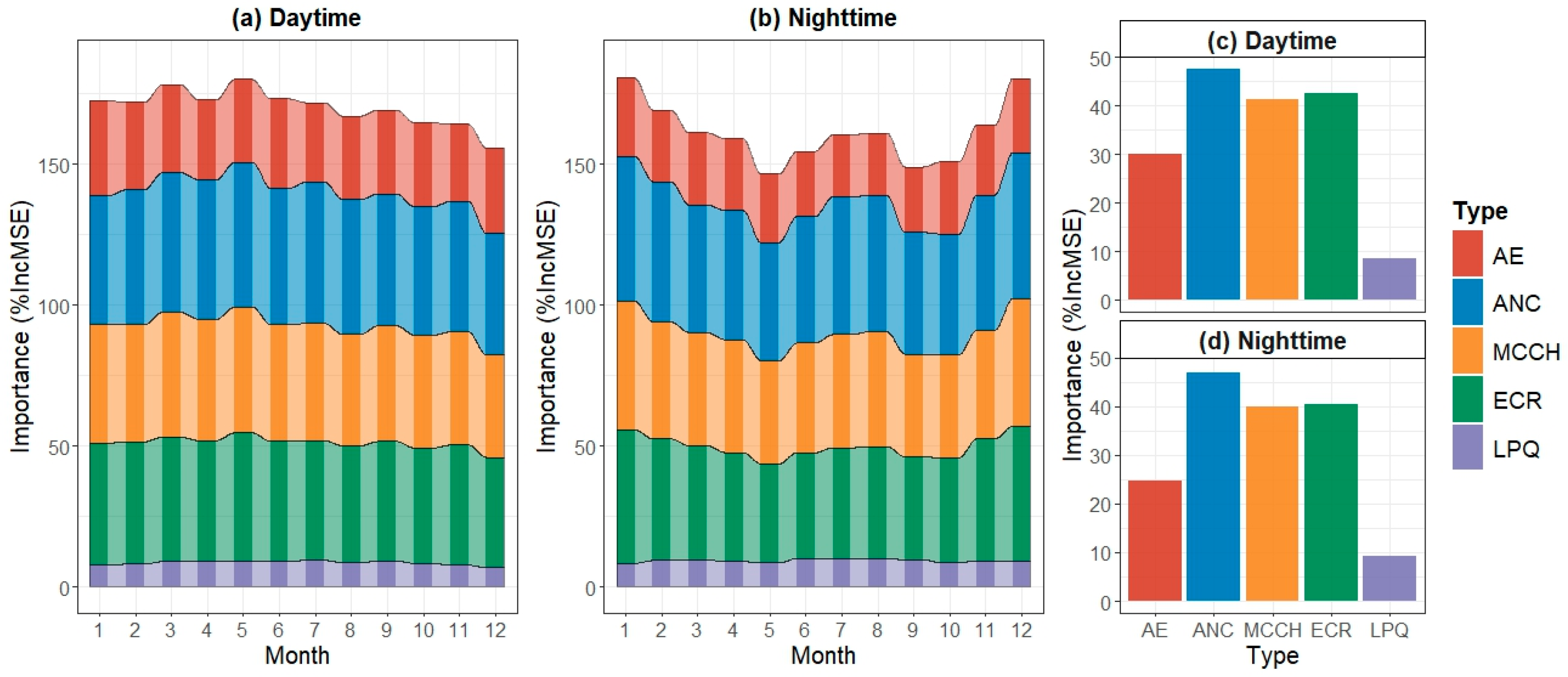
| Average Elevation (AE) | AE is the average elevation in the section elevation series of a single direction. It is mainly used to illustrate the elevation where terrain blockage occurs. It is calculated as the statistical mean according to the values of section elevation series and is a global feature of terrain blockage. |
| Average Neighbor Change (ANC) | ANC is the average value of all local changes in the section elevation series of a single direction and characterizes the difficulty of near-surface air in moving from one location to a neighboring location. A larger ANC indicates higher difficulty of short-distance movement for near-surface air. ANC is a local feature of terrain blockage. |
| Elevation Changing Range (ECR) | ECR is the global range of elevation in the section elevation series of a single direction. ECR equals the difference between the maximum and the minimum elevation in a single direction. A larger ECR indicates that it is more difficult for near-surface air to realize long-distance movement and is a global feature of terrain blockage. |
| Maximum Continuous Climbing Height (MCCH) | MCCH is the height difference in a part of section elevation series and represents the longest distance when elevation is continuously increasing. The continuous increase in elevation means the continuous climbing of near-surface air, which needs to overcome the barrier of terrain. Thus, MCCH is the largest barrier of terrain in the process of near-surface air movement and is a local feature of terrain blockage. |
| Local Peak Quantity (LPQ) | LPQ is the quantity of local mountain peak in the section elevation series of a single direction. LPQ reflect the number of times near-surface air needs to overcome the barrier of terrain to climb and is a global feature of terrain blockage. The minimum value of LPQ is zero. |
| Terrain Blockage Features (TBFs) | Traditional Terrain Features | |||
|---|---|---|---|---|
| Average | Standard Deviation | Average | Standard Deviation | |
| R-squared | 0.8834 | 0.0161 | 0.8474 | 0.0215 |
| RMSE | 1.6418 | 0.2350 | 1.8771 | 0.2654 |
| MAE | 1.2257 | 0.1511 | 1.4140 | 0.1753 |
| MD | −0.007 | 0.015 | −0.002 | 0.005 |
Disclaimer/Publisher’s Note: The statements, opinions and data contained in all publications are solely those of the individual author(s) and contributor(s) and not of MDPI and/or the editor(s). MDPI and/or the editor(s) disclaim responsibility for any injury to people or property resulting from any ideas, methods, instructions or products referred to in the content. |
© 2024 by the authors. Licensee MDPI, Basel, Switzerland. This article is an open access article distributed under the terms and conditions of the Creative Commons Attribution (CC BY) license (https://creativecommons.org/licenses/by/4.0/).
Share and Cite
Gao, H.; Dong, Y.; Zhou, L.; Wang, X. Exploring the Influence of Terrain Blockage on Spatiotemporal Variations in Land Surface Temperature from the Perspective of Heat Energy Redistribution. ISPRS Int. J. Geo-Inf. 2024, 13, 200. https://doi.org/10.3390/ijgi13060200
Gao H, Dong Y, Zhou L, Wang X. Exploring the Influence of Terrain Blockage on Spatiotemporal Variations in Land Surface Temperature from the Perspective of Heat Energy Redistribution. ISPRS International Journal of Geo-Information. 2024; 13(6):200. https://doi.org/10.3390/ijgi13060200
Chicago/Turabian StyleGao, Hong, Yong Dong, Liang Zhou, and Xi Wang. 2024. "Exploring the Influence of Terrain Blockage on Spatiotemporal Variations in Land Surface Temperature from the Perspective of Heat Energy Redistribution" ISPRS International Journal of Geo-Information 13, no. 6: 200. https://doi.org/10.3390/ijgi13060200