
Soil and Regulated Deficit Irrigation Affect Growth, Yield and Quality of ‘Nero d’Avola’ Grapes in a Semi-Arid Environment


 and
and 
Abstract
1. Introduction
2. Materials and Methods
2.1. Experimental Site
2.2. Soil Characteristics
2.3. Irrigation Treatments
2.4. Experimental Design
2.5. Soil Water Content
2.6. Ecophysilogical Measurements
2.7. Leaf Area and Pruning Mass
2.8. Yield and Grape Composition
2.9. Statistical Analysis
3. Results and Discussion
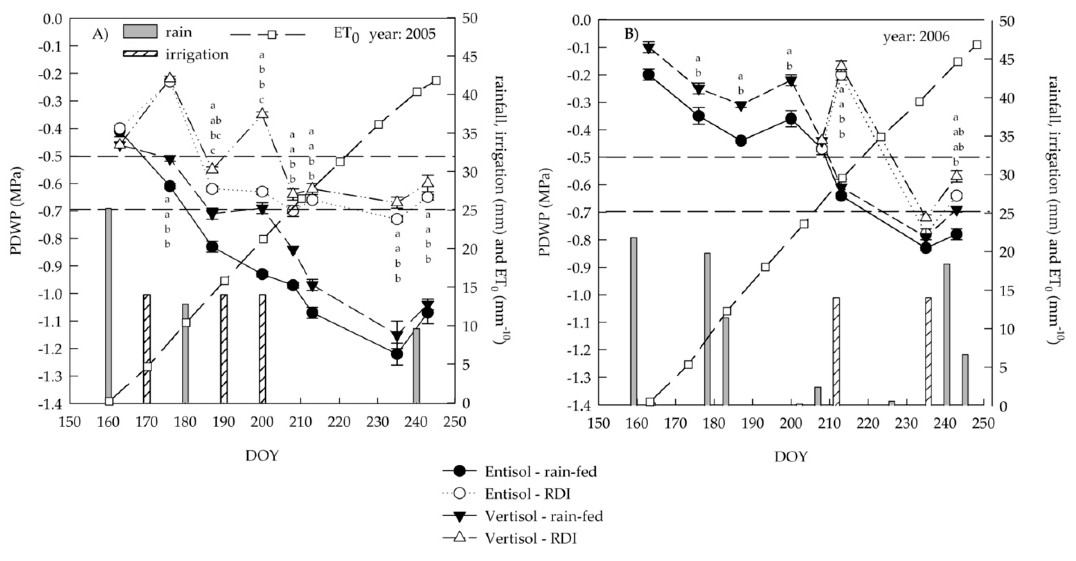
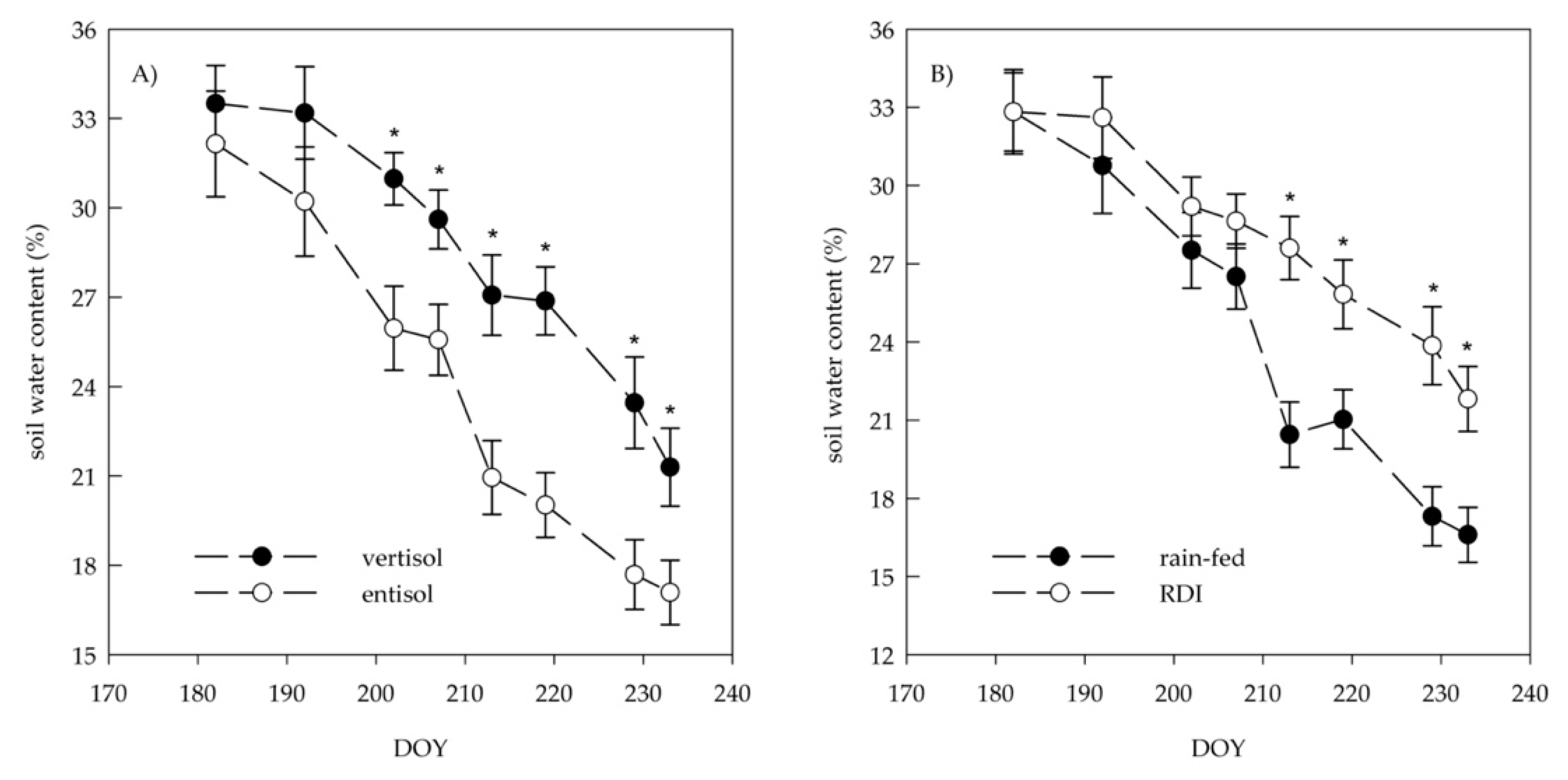
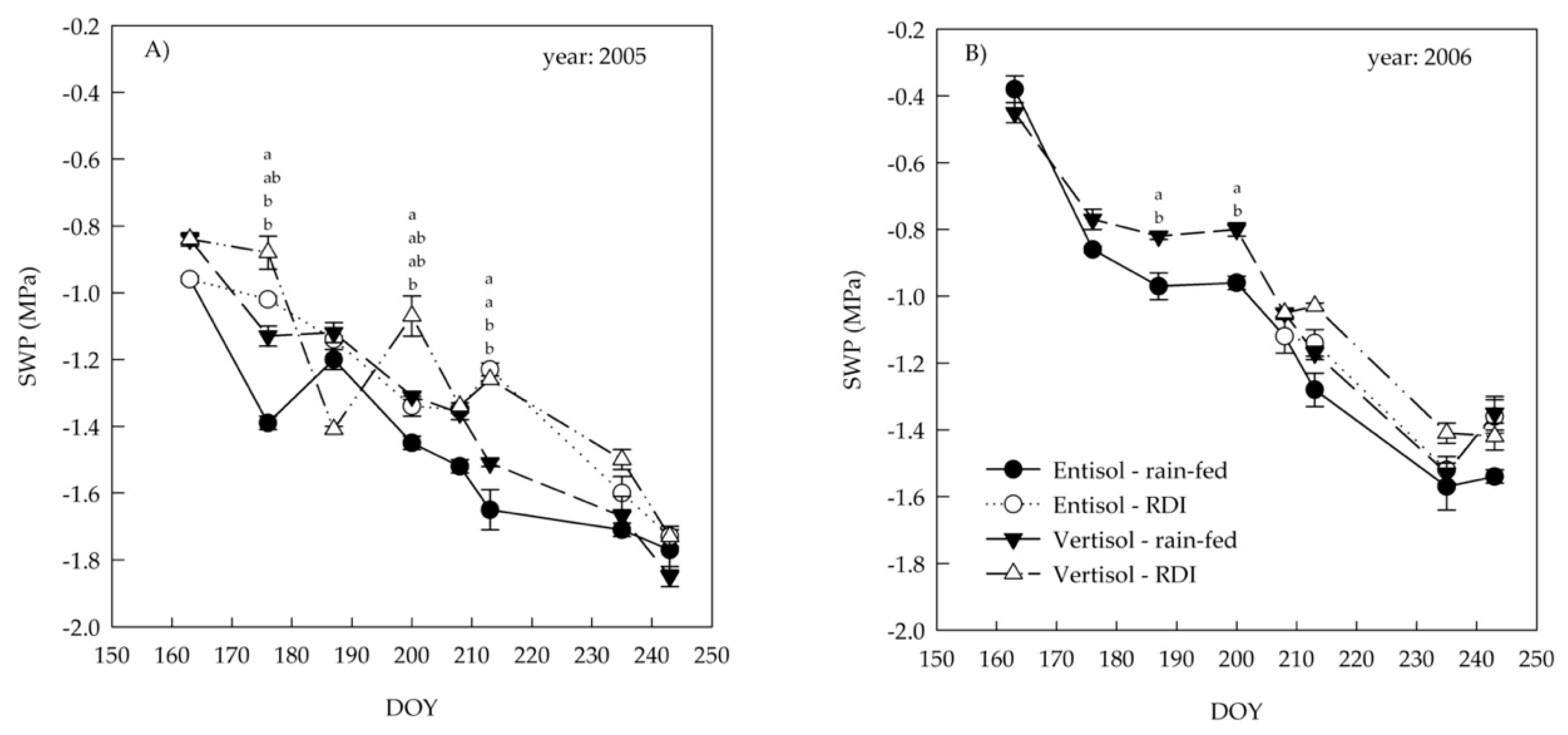
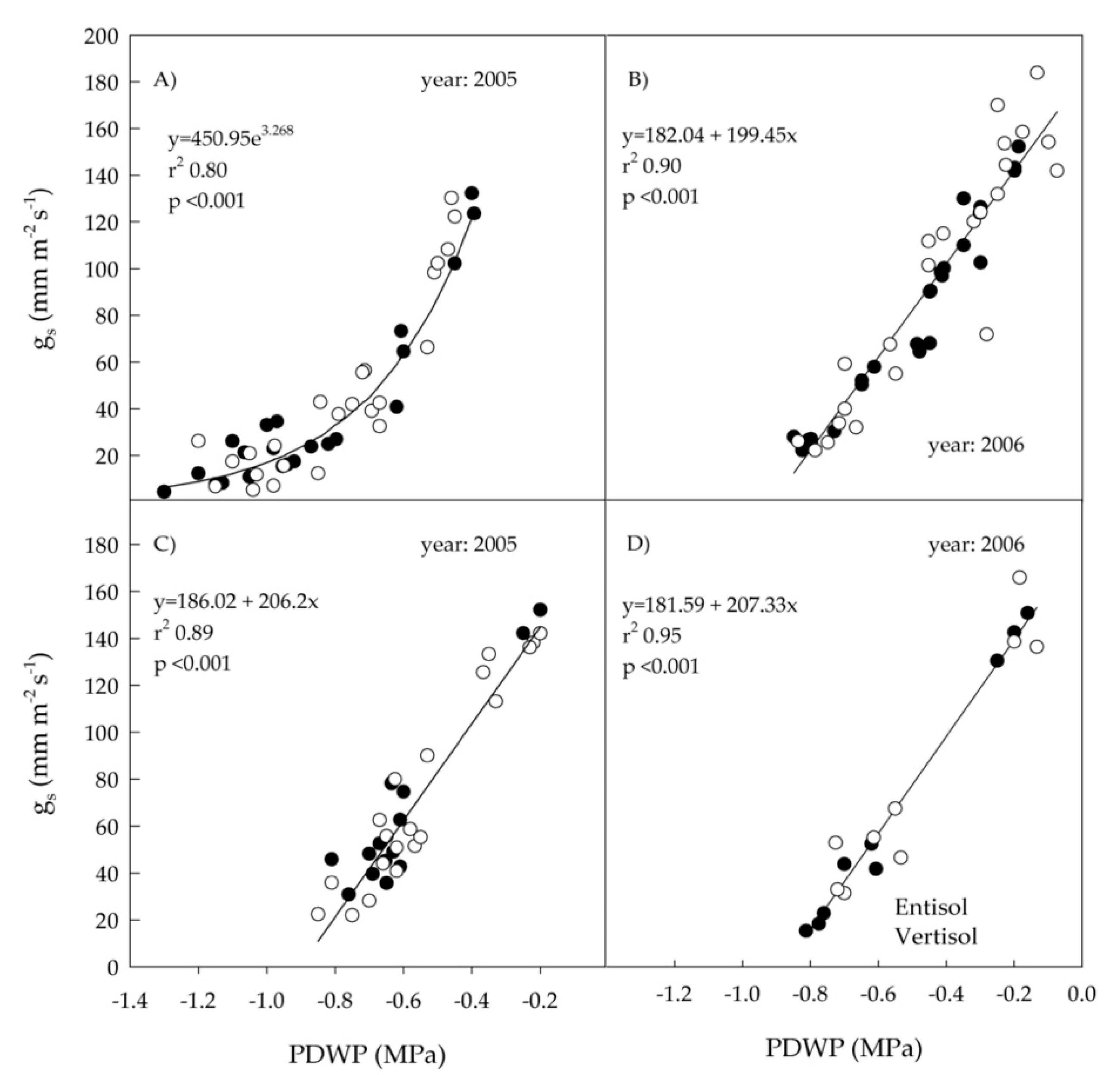
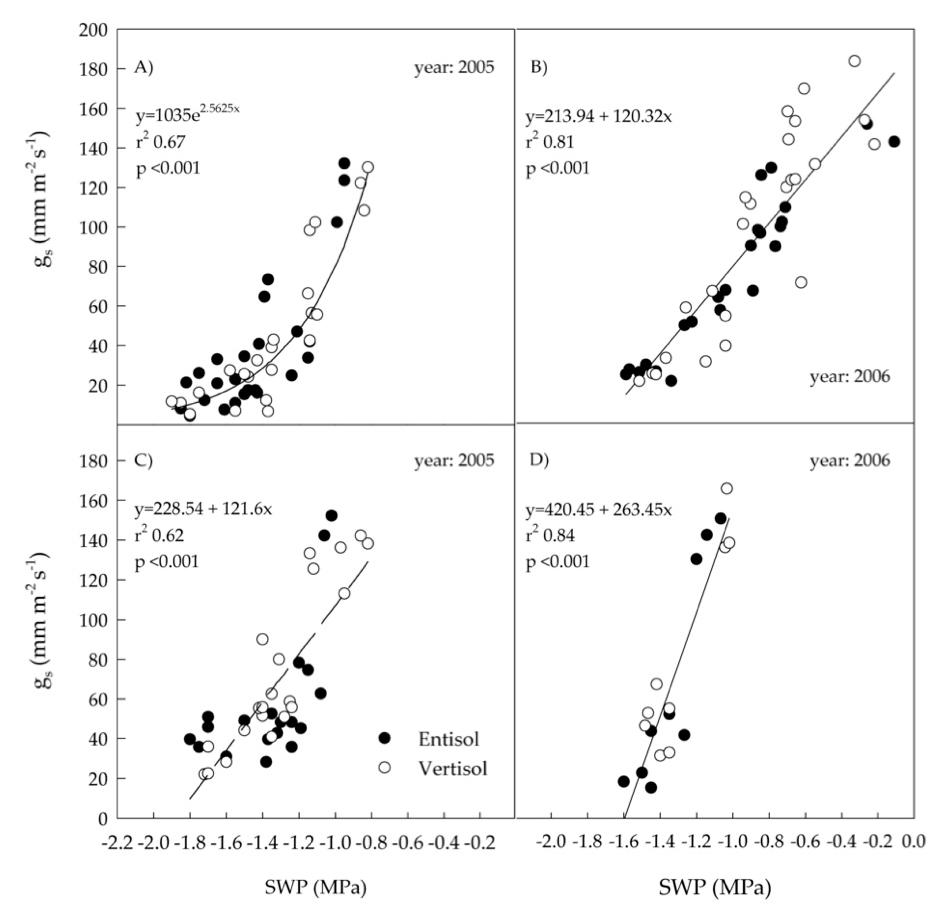
3.1. Meteorological Conditions, Soil Water Content and Ecophysilogical Measurements
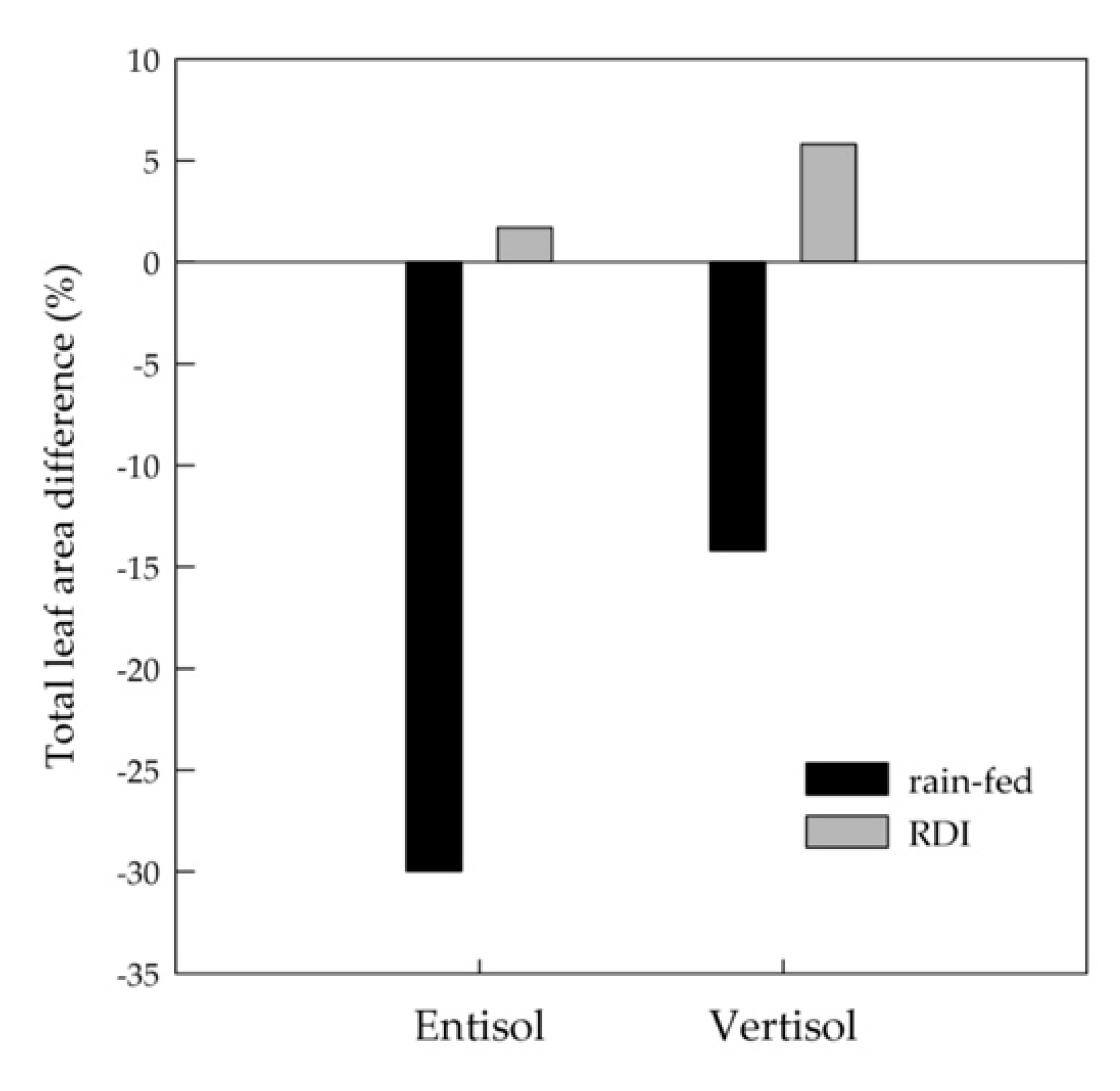
3.2. Leaf Area and Cane Mass
3.3. Yield and Grape Composition
4. Conclusions
Supplementary Materials
Author Contributions
Funding
Institutional Review Board Statement
Informed Consent Statement
Data Availability Statement
Acknowledgments
Conflicts of Interest
Abbreviations
References
- Giorgi, F.; Lionello, P. Climate change projections for the Mediterranean region. Glob. Planet. Chang. 2008, 63, 90–104. [Google Scholar] [CrossRef]
- IPCC. Climate Change 2014: Impacts, Adaptation, and Vulnerability; IPCC: Cambridge, UK; New York, NY, USA, 2014. [Google Scholar]
- Santos, J.A.; Fraga, H.; Malheiro, A.C.; Moutinho-Pereira, J.; Dinis, L.T.; Correia, C.; Moriondo, M.; Leolini, L.; Dibari, C.; Costafreda-Aumedes, S.; et al. A Review of the Potential Climate Change Impacts and Adaptation Options for European Viticulture. Appl. Sci. 2020, 10, 3092. [Google Scholar] [CrossRef]
- van Leeuwen, C.; de Rességuier, L. Major Soil-Related Factors in Terroir Expression and Vineyard Siting. Elements 2018, 14, 159–165. [Google Scholar] [CrossRef]
- van Leeuwen, C. Terroir: The effect of the physical environment on vine growth, grape ripening and wine sensory attributes. In Managing Wine Quality. Volume 1: Viticulture and Wine Quality; Reynolds, A., Ed.; Woodhead Publishing Ltd.: Oxford, UK, 2010; pp. 273–315. [Google Scholar] [CrossRef]
- Seguin, G. Alimentation en eau de la vigne et composition chimique des moûts dans les grands crus du Médoc. Phénomènes de régulation. J. Int. Sci. Vigne Vin. 1975, 9, 23–34. [Google Scholar] [CrossRef]
- Willwerth, J.J.; Reynolds, A.G.; Lesschaeve, I. Sensory analysis of Ontario Riesling wines from various water status zones. OENO One 2018, 52, 145–171. [Google Scholar] [CrossRef]
- Reynolds, A.G.; Taylor, G.; de Savigny, C. Defining Niagara terroir by chemical and sensory analysis of Chardonnay wines from various soil textures and vine sizes. Am. J. Enol. Vitic. 2013, 64, 180–194. [Google Scholar] [CrossRef]
- van Leeuwen, C.; Friant, P.; Choné, X.; Tregoat, O.; Koundouras, S.; Dubourdieu, D. Influence of climate, soil, and cultivar on terroir. Am. J. Enol. Vitic. 2004, 55, 207–217. [Google Scholar]
- Fraga, H.; García de Cortázar Atauri, I.; Santos, J.A. Viticultural irrigation demands under climate change scenarios in Portugal. Agric. Water Manag. 2018, 196, 66–74. [Google Scholar] [CrossRef]
- Hunter, J.J.; Volschenk, C.G.; Novello, V.; Pisciotta, A.; Booyse, M.; Fouché, G.W. Integrative effects of vine water relations and grape ripeness level of Vitis vinifera L. cv. Shiraz/Richter 99. II. Grape composition and wine quality. S. Afr. J. Enol. Vitic. 2014, 35, 359–374. [Google Scholar] [CrossRef][Green Version]
- Zufferey, V.; Verdenal, T.; Dienes, A.; Belcher, S.; Lorenzini, F.; Koestel, C.; Blackford, M.; Bourdin, G.; Gindro, K.E.; Spangenberg, J.; et al. The influence of vine water regime on the leaf gas exchange, berry composition and wine quality of Arvine grapes in Switzerland. OENO 2020, 3, 553–568. [Google Scholar] [CrossRef]
- Castellarin, S.D.; Pfeiffer, A.; Sivilotti, P.; Degan, M.; Peterlunger, E.; Di Gaspero, G. Transcriptional regulation of anthocyan biosynthesis in ripening fruits pf grapevine under seasonal water deficit. Plant Cell Environ. 2007, 30, 1381–1399. [Google Scholar] [CrossRef] [PubMed]
- Castellarin, S.D.; Matthews, M.A.; Di Gaspero, G.; Gambetta, G.A. Water deficits accelerate ripening and induce changes in gene expression regulating flavonoid biosynthesis in grape berries. Planta 2007, 227, 101–112. [Google Scholar] [CrossRef]
- Ojeda, H.; Andary, C.; Kraeva, E.; Carbonneau, A.; Deloire, A. Influence of pre- and postveraison water deficit on synthesis and concentration of skin phenolic compounds during berry growth of Vitis vinifera cv. Shiraz. Am. J. Enol. Vitic. 2002, 53, 261–267. [Google Scholar]
- Roby, G.; Matthews, M.A. Relative proportions of seed; skin and flesh; in ripe berries from Cabernet Sauvignon grapevines grown in a vineyard either well irrigated or under water deficit. Austr. J. Grape Wine Res. 2004, 10, 74–84. [Google Scholar] [CrossRef]
- Barbagallo, M.G.; Guidoni, S.; Hunter, J.J. Berry size and qualitative characteristics of Vitis vinifera L. cv. Syrah. S. Afr. J. Enol. Vitic. 2011, 32, 129–136. [Google Scholar] [CrossRef]
- Girona, J.; Mata, M.; del Campo, J.; Arbonés, A.; Bartra, E.; Marsal, J. The use of midday leaf water potential for scheduling deficit irrigation in vineyards. Irrig. Sci. 2006, 24, 115–127. [Google Scholar] [CrossRef]
- Allen, R.G.; Pereira, L.S.; Raes, D.; Smith, M. Crop Evapotranspiration: Guidelines for Computing Crop Water Requirements; Irrigation and Drainage 56; FAO: Rome, Italy, 1998. [Google Scholar]
- Reynolds, A.G.; Naylor, A.P. ‘‘Pinot noir’’ and ‘‘Riesling’’ grapevines respond to water stress duration and soil water holding capacity. Hort. Sci. 1994, 29, 1505–1510. [Google Scholar] [CrossRef]
- Montoro, A.; Fereres, E.; Lopez-Urrea, R.; Manas, F.; Lopez-Fuster, P. Sensitivity of trunk diameter fluctuations in Vitis vinifera L. Tempranillo and Cabernet Sauvignon cultivars. Am. J. Enol. Vitic. 2012, 63, 85–93. [Google Scholar] [CrossRef]
- Belfiore, N.; Vinti, R.; Lovat, L.; Chitarra, W.; de Bei, R.; Meggio, F.; Gaiotti, F. Infrared Thermography to Estimate Vine Water Status: Optimizing Canopy Measurements and Thermal Indices for the Varieties Merlot and Moscato in Northern Italy. Agronomy 2019, 9, 821. [Google Scholar] [CrossRef]
- Williams, L.E.; Araujo, F.J. Correlations among predawn leaf; midday leaf and midday stem water potential and their correlations with other measures of soil and plant water status in Vitis vinifera. J. Amer. Soc. Hort. Sci. 2002, 127, 448–454. [Google Scholar] [CrossRef]
- Santesteban, L.G.; Miranda, C.; Royo, J.B. Suitability of pre-dawn and stem water potential as indicators of vineyard water status in cv. Tempranillo. Aust. J. Grape Wine Res. 2011, 17, 43–51. [Google Scholar] [CrossRef]
- Carbonneau, A.; Deloire, A.; Costanza, P. Le potentiel hydrique foliaire: Sens des différentes modalités de mesure. J. Int. Sci. Vigne Vin. 2004, 38, 15–19. [Google Scholar] [CrossRef]
- Intrigliolo, D.S.; Castel, J.R. Vine and soil-based measures of water status in a Tempranillo vineyard. Vitis 2006, 45, 157–163. [Google Scholar] [CrossRef]
- Chonè, X.; van Leeuwen, C.; Dubourdieu, D.; Gaudillére, J.P. Stem water potential is a sensitive indicator of grapevine water status. Ann. Bot. 2001, 87, 477–483. [Google Scholar] [CrossRef]
- Williams, L.E.; Trout, T.J. Relationships among vine- and soil-based measures of water status in a Thompson Seedless vineyard in response to high-frequency drip irrigation. Am. J. Enol. Vitic. 2005, 56, 357–366. [Google Scholar]
- Schultz, H.R. Differences in hydraulic architecture account for near-isohydric and anisohydric behaviour of two field-grown Vitis vinifera L. cultivars during drought. Plant Cell Environ. 2003, 26, 1393–1405. [Google Scholar] [CrossRef]
- AAVV. Nero d’Avola (Calabrese). In Identità e Ricchezza del Vigneto Sicilia; Regione Siciliana; Assessorato dell’Agricoltura, dello Sviluppo Rurale e della Pesca Mediterranea (Ed.): Palermo, Italy, 2014; pp. 114–120. [Google Scholar]
- AAVV. Composizione Varietale del “Vigneto Sicilia”; Regione Siciliana; Istituto Regionale della Vite e del Vino. IRVO (Ed.): Palermo, Italy, 2020. [Google Scholar]
- AAVV. I Numeri del Nero d’Avola; Regione Siciliana; Istituto Regionale della Vite e del Vino: IRVO (Ed.: Palermo, Italy, 2020. [Google Scholar]
- Oddo, E.; Abbate, L.; Inzerillo, S.; Carimi, F.; Motisi, A.; Sajeva, M.; Nardini, A. Water relations of two Sicilian grapevine cultivars in response to potassium availability and drought stress. Plant Physiol. Biochem. 2020, 148, 282–290. [Google Scholar] [CrossRef] [PubMed]
- United States Department of Agriculture (USDA). Soil Taxonomy, a Basic System of Soil Classification for Making and Interpreting Soil Surveys, 2nd ed.; Agricultural Handbook; Soil Survey Staff (Ed.): Washington, DC, USA, 1999; No. 436. [Google Scholar]
- Richards, L.A. Pressure-membrane apparatus construction and use. Agric. Eng. 1947, 28, 451–454. [Google Scholar]
- Scholander, P.F.; Bradstreet, E.D.; Hemmingsen, E.A.; Hammel, H.T. Sap pressure in vascular plants. Science 1965, 148, 339–346. [Google Scholar] [CrossRef]
- Di Stefano, R.; Cravero, M.C. Metodi per lo studio dei polifenoli dell’uva. Riv. Vitic. Enol. 1991, 2, 37–45. [Google Scholar]
- R Core Team. R: A Language and Environment for Statistical Computing; R Foundation for Statistical Computing: Vienna, Austria, 2020; Available online: https://www.R-project.org/ (accessed on 27 March 2021).
- Bates, D.; Maechler, M.; Bolker, B.; Walker, S. Fitting Linear Mixed-Effects Models Using lme4. J. Stat. Softw. 2015, 67, 1–48. [Google Scholar] [CrossRef]
- Barbagallo, M.G.; Costanza, P.; Di Lorenzo, R.; Gugliotta, E.; Pisciotta, A.; Raimondi, S.; Santangelo, T. Effect of Irrigation and Soil Type on Root Growth and Distribution of Vitis Vinifera L. cv Nero d’Avola Grown in Sicily; Elsevier B.V.: Amsterdam, The Netherlands, 2004; pp. 444–451. [Google Scholar]
- Tramontini, S.; van Leeuwen, C.; Domec, J.C.; Destrac-Irvine, A.; Basteau, C.; Vitali, M.; Mosbach-Schulz, O.; Lovisolo, C. Impact of soil texture and water availability on the hydraulic control of plant and grape-berry development. Plant Soil 2013, 368, 215–230. [Google Scholar] [CrossRef]
- Cifre, J.; Bota, J.; Escalona, J.M.; Medrano, H.; Flexas, J. Physiological tools for irrigation scheduling in grapevine (Vitis vinifera L.) An open gate to improve water-use efficiency? Agric. Ecosyst. Environ. 2005, 106, 159–170. [Google Scholar] [CrossRef]
- Lovisolo, C.; Perrone, I.; Carra, A.; Ferrandino, A.; Flexas, J.; Medrano, H.; Schubert, A. Drought-induced changes in development and function of grapevine (Vitis spp.) organs and in their hydraulic and non-hydraulic interactions at the whole-plant level: A physiological and molecular update. Funct. Plant Biol. 2010, 37, 98–116. [Google Scholar] [CrossRef]
- Novara, A.; Pisciotta, A.; Minacapilli, M.; Maltese, A.; Capodici, F.; Cerdà, A.; Gristina, L. The impact of soil erosion on soil fertility and vine vigor. A multidisciplinary approach based on field, laboratory and remote sensing approaches. Sci. Total Environ. 2018, 622–623, 474–480. [Google Scholar] [CrossRef]
- Brillante, L.; Mathieu, O.; Bois, B.; van Leeuwen, C.; Lévêque, J. The use of soil electrical resistivity to monitor plant and soil water relationships in vineyards. Soil 2015, 1, 273–286. [Google Scholar] [CrossRef]
- Brenot, J.; Quiquerez, A.; Petit, C.; Garcia, J.P. Erosion rates and sediment budgets in vineyards at 1-m resolution based on stock unearthing (Burgundy, France). Geomorphology 2008, 100, 345–355. [Google Scholar] [CrossRef]
- Hochberg, U.; Bonel, A.G.; David-Schwartz, R.; Degu, A.; Fait, A.; Cochard, H.; Peterlunger, E.; Herrera, J.C. Grapevine acclimation to water deficit: The adjustment of stomatal and hydraulic conductance differs from petiole embolism vulnerability. Planta 2017, 245, 1091–1104. [Google Scholar] [CrossRef]
- Ginestar, C.; Eastham, J.; Gray, S.; Iland, P. Use of sap-flow sensors to schedule vineyard irrigation. I. Effects of post-veraison water deficits on water relations; vine growth; and yield of Shiraz grapevines. Am. J. Enol. Vitic. 1998, 49, 413–420. [Google Scholar]
- Keller, M. Deficit irrigation and vine mineral nutrition. Am. J. Enol. Vitic. 2005, 56, 267–283. [Google Scholar]
- Merli, M.C.; Gatti, M.; Galbignani, M.; Bernizzoni, F.; Magnanini, E.; Poni, S. Comparison of whole-canopy water use efficiency and vine performance of cv: Sangiovese (Vitis vinifera L.) vines subjected to a post-veraison water deficit. Sci. Hort. 2015, 185, 113–120. [Google Scholar] [CrossRef]
- Romero, P.; Fernández-Fernández, J.I.; Martinez-Cutillas, A. Physiological thresholds for efficient regulated deficit-irrigation management in winegrapes grown under semiarid conditions. Am. J. Enol. Vitic. 2010, 61, 300–312. [Google Scholar]
- Di Lorenzo, R.; Sottile, I.; Barbagallo, M.G.; Occorso, G.; Iannolino, G.; Meli, R. Influenza delle forme di allevamento sull’andamento della superficie fogliare della vite in Sicilia. In Proceeding for the Fourth International Symposium on Vine Physiology; San Michele all’Adige: Torino, Italy, 1992; pp. 75–80. [Google Scholar]
- Shelden, M.C.; Vandeleur, R.; Kaiser, B.N.; Tyerman, S.D. A Comparison of Petiole Hydraulics and Aquaporin Expression in an Anisohydric and Isohydric Cultivar of Grapevine in Response to Water-Stress Induced Cavitation. Frontiers in Plant Science 2017, 8, 1893. [Google Scholar] [CrossRef] [PubMed]
- Palliotti, A.; Silvestroni, O.; Petoumenou, D. Photosynthetic and photoinhibition behavior of two field-grown grapevine cultivars under multiple summer stresses. Am. J. Enol. Vitic. 2009, 60, 189–198. [Google Scholar]
- Sivilotti, P.; Sonetto, C.; Paladin, M.; Peterlunger, E. Effect of Soil Moisture Availability on Merlot: From Leaf Water Potential to Grape Composition. Am. J. Enol. Vitic. 2005, 56, 9–18. [Google Scholar]
- Mirás-Avalos, J.M.; Intrigliolo, D.S. Grape Composition under Abiotic Constrains: Water Stress and Salinity. Front. Plant Sci. 2017, 8, 851. [Google Scholar] [CrossRef] [PubMed]
- Triolo, R.; Roby, J.P.; Pisciotta, A.; Di Lorenzo, R.; van Leeuwen, C. Impact of vine water status on berry mass and berry tissue development of Cabernet franc (Vitis vinifera L.), assessed at berry level. J. Sci. Food Agric. 2019, 9, 5711–5719. [Google Scholar] [CrossRef]
- Chaves, M.M.; Zarrouk, O.; Francisco, R.; Costa, J.M.; Santos, T.; Regalado, A.P.; Rodrigues, M.L.; Lopes, C.M. Grapevine under deficit irrigation: Hints from physiological and molecular data. Ann. Bot. 2010, 105, 661–676. [Google Scholar] [CrossRef]
- Basile, B.; Marsal, J.; Mata, M.; Vallverdú, X.; Bellvert, J.; Girona, J. Phenological sensitivity of Cabernet Sauvignon to water stress: Vine physiology and berry composition. Am. J. Enol. Vitic. 2011, 62, 452–461. [Google Scholar] [CrossRef]
- Bindon, K.A.; Dry, P.R.; Loveys, B.R. The interactive effect of pruning level and irrigation strategy on grape berry ripening and composition in Vitis vinifera L. cv. Shiraz. S. Afr. J. Enol. Vitic. 2008, 29, 71–78. [Google Scholar] [CrossRef]
- Bowen, P.; Bogdanoff, C.; Usher, K.; Estergaard, B.; Watson, M. Effects of irrigation and crop load on leaf gas exchange and fruit composition in red winegrapes grown on a loamy sand. Am. J. Enol. Vitic. 2011, 62, 9–22. [Google Scholar] [CrossRef]
- Deluc, L.G.; Quilici, D.R.; Decendit, A.; Grimplet, J.; Wheatley, M.D.; Schlauch, K.A.; Mérillon, J.M.; Cushman, J.C.; Cramer, G.R. Water deficit alters differentially metabolic pathways affecting important flavor and quality traits in grape berries of Cabernet Sauvignon and Chardonnay. BMC Genom. 2009, 10, 212–245. [Google Scholar] [CrossRef]
- Gaudillère, J.P.; van Leeuwen, C.; Ollat, N. Carbon isotope composition of sugars in grapevine; an integrated indicator of vineyard water status. J. Exp. Bot. 2002, 53, 757–763. [Google Scholar] [CrossRef] [PubMed]
- Intrigliolo, D.S.; Castel, J.R. Response of grapevine cv. ‘Tempranillo’ to timing and amount of irrigation: Water relations, vine growth, yield and berry and wine composition. Irrig. Sci. 2010, 28, 113–125. [Google Scholar] [CrossRef]
- Myburgh, P.A. Water status, vegetative growth and yield responses of Vitis vinifera L. cvs. Sauvignon blanc and Chenin blanc to timing of irrigation during berry ripening in the coastal region of South Africa. S. Afr. J. Enol. Vitic. 2005, 26, 59–67. [Google Scholar] [CrossRef][Green Version]
- Chapman, D.M.; Roby, G.; Ebeler, S.E.; Guinard, J.X.; Matthews, M.A. Sensory attributes of Cabernet Sauvignon wines made from vines with different water status. Aust. J. Grape Wine Res. 2005, 11, 339–347. [Google Scholar] [CrossRef]
- Estaban, M.A.; Villanueva, M.J.; Lissarrague, J.R. Effect of irrigation on changes in berry composition during maturation. Sugars; organic acids; and mineral elements. Am. J. Enol. Vitic. 1999, 50, 418–434. [Google Scholar]
- Etchebarne, F.; Ojeda, H.; Hunter, J.J. Leaf:Fruit Ratio and Vine Water Status Effects on Grenache Noir (Vitis vinifera L.) Berry Composition: Water, Sugar, Organic Acids and Cations. S. Afr. J. Enol. Vitic. 2010, 31, 106–115. [Google Scholar] [CrossRef][Green Version]
- Morris, J.R.; Cawthon, D.L. Effect of irrigation; fruit load; and potassium fertilization on yield; quality and petiole analysis of Concord (Vitis labrusca L.) grapes. Am. J. Enol. Vitic. 1982, 33, 145–148. [Google Scholar]
- Mpelasoka, B.S.; Schachtman, D.P.; Treeby, M.L.T.; Thomas, M.R. A review of potassium nutrition in grapevines with special emphasis on berry accumulation. Aust. J. Grape Wine Res. 2003, 9, 154–168. [Google Scholar] [CrossRef]
- Boss, P.K.; Davies, C.; Robinson, S.P. Analysis of the expression of anthocyanin pathway genes in developing Vitis vinifera L. cv. Shiraz grape berries and the implications for pathway regulation. Plant Physiol. 1996, 111, 1059–1066. [Google Scholar] [CrossRef] [PubMed]
- Girona, J.; Marsal, J.; Mata, M.; del Campo, J.; Basile, B. Phenological sensitivity of berry growth and composition of Tempranillo grapevines (Vitis vinifera L.) to water stress. Aust. J. Grape. Wine Res. 2009, 15, 268–277. [Google Scholar] [CrossRef]


| Year | Month | Jan | Feb | Mar | Apr | May | Jun | Jul | Aug | Sep | Oct | Nov | Dec |
|---|---|---|---|---|---|---|---|---|---|---|---|---|---|
| T min (°C) | 4.80 | 3.42 | 7.07 | 8.78 | 13.81 | 17.24 | 20.30 | 18.68 | 17.18 | 13.99 | 9.64 | 6.09 | |
| 2005 | T max (°C) | 9.76 | 9.10 | 15.10 | 16.33 | 24.28 | 27.93 | 31.33 | 29.88 | 27.07 | 22.93 | 17.51 | 11.97 |
| rainfall (mm) | 88.8 | 77.2 | 55.20 | 121.8 | 13.4 | 40.2 | 12.80 | 16.00 | 29.80 | 88.00 | 82.60 | 107.8 | |
| Et0 (mm) | 0.89 | 1.25 | 2.30 | 2.74 | 4.43 | 4.89 | 5.32 | 4.38 | 3.04 | 1.76 | 1.16 | 0.86 | |
| T min (°C) | 4.76 | 5.20 | 6.73 | 10.60 | 14.32 | 17.25 | 19.76 | 19.44 | 17.12 | 15.49 | 10.58 | 9.02 | |
| 2006 | T max (°C) | 10.58 | 12.03 | 14.29 | 19.88 | 25.42 | 26.06 | 30.22 | 30.38 | 26.11 | 23.25 | 18.16 | 15.67 |
| rainfall (mm) | 73.60 | 57.20 | 44.80 | 41.20 | 18.60 | 22.20 | 31.20 | 3.20 | 97.00 | 30.00 | 29.80 | 79.60 | |
| Et0 (mm) | 0.88 | 1.34 | 2.15 | 3.31 | 4.64 | 5.28 | 5.75 | 4.94 | 3.23 | 2.27 | 1.47 | 0.87 |
| Year | 2005 | 2006 | 2005 | 2006 | |
|---|---|---|---|---|---|
| Soil | Irrigation | Rain-Fed | RDI | ||
| Entisol | b1 | 0.922 | 1.655 | 0.952 | 0.629 |
| SEb | 0.11 | 0.11 | 0.25 | 0.09 | |
| r2 | 0.77 | 0.95 | 0.44 | 0.86 | |
| p-value | <0.001 | <0.001 | <0.001 | <0.001 | |
| Vertisol | b1 | 1.084 | 1.398 | 1.264 | 0.725 |
| SEb | 0.15 | 0.09 | 0.11 | 0.12 | |
| r2 | 0.70 | 0.92 | 0.87 | 0.83 | |
| p-value | <0.001 | <0.001 | <0.001 | <0.001 | |
| Student’s t-test | t-value | 0.870 | 1.874 | 1.150 | 0.611 |
| p-value | 0.39 | 0.07 | 0.26 | 0.55 | |
| Year | 2005 | 2006 | ||
|---|---|---|---|---|
| Irrigation | Rain-Fed | RDI | Rain-Fed | RDI |
| b1 | 1.006 | 1.122 | 1.498 | 0.676 |
| SEb | 0.009 | 0.127 | 0.076 | 0.073 |
| r2 | 0.79 | 0.66 | 0.91 | 0.84 |
| p value | <0.001 | <0.001 | <0.001 | 0.001 |
| t-value | p-value | ||
|---|---|---|---|
| rain-fed | 2005 vs. 2006 | 6.428 | 0.000 |
| RDI | 2005 vs. 2006 | 3.045 | 0.003 |
| 2005 | rain-fed vs. RDI | 0.911 | 0.366 |
| 2006 | rain-fed vs. RDI | 7.800 | 0.000 |
| TLA | Cane | Yield | Cluster | Berry | |
|---|---|---|---|---|---|
| (cm2/shoot) | (g) | (kg/vine) | (g) | (g) | |
| Soil | |||||
| Entisol | 4233 ± 169 | 58.0 ± 5.0 | 2.41 ± 0.14 | 198 ± 9.0 | 1.51 ± 0.01 |
| Vertisol | 4909 ± 170 | 79.0 ± 8.0 | 3.36 ± 0.19 | 278 ± 25 | 1.76 ± 0.03 |
| Irrigation | |||||
| Rain-fed | 4071 ± 244 | 64.0 ± 6.0 | 2.68 ± 0.14 | 220 ± 19 | 1.48 ± 0.01 |
| RDI | 5071 ± 345 | 73.0 ± 7.0 | 3.09 ± 0.17 | 257 ± 14 | 1.79 ± 0.02 |
| Main factors | p-value | p-value | p-value | p-value | p-value |
| Soil (S) | <0.001 | <0.001 | 0.001 | 0.008 | 0.012 |
| Irrigation (I) | <0.001 | 0.065 | 0.007 | 0.011 | <0.001 |
| Interaction | |||||
| S × I | 0.207 | 0.155 | 0.954 | 0.749 | 0.052 |
| TSS | TA | Anthocyanin | Anthocyanin | |
|---|---|---|---|---|
| (°Brix) | (g L−1) | (mg kg−1) | (mg/berry) | |
| Soil | ||||
| Entisol | 22.70 ± 0.15 | 6.62 ± 0.07 | 1293 ± 41 | 1.92 ± 0.09 |
| Vertisol | 22.90 ± 0.17 | 6.94 ± 0.12 | 1169 ± 65 | 2.02 ± 0.07 |
| Irrigation | ||||
| Rain-fed | 22.85 ± 0.11 | 7.15 ± 0.09 | 1343 ± 52 | 1.97 ± 0.09 |
| RDI | 22.75 ± 0.21 | 6.41 ± 0.10 | 1119 ± 54 | 1.97 ± 0.06 |
| Main factors | p-value | p-value | p-value | p-value |
| Soil (S) | 0.306 | 0.045 | 0.040 | 0.412 |
| Irrigation (I) | 0.451 | <0.001 | <0.001 | 0.971 |
| Interaction | ||||
| S × I | 0.640 | 0.154 | 0.197 | 0.651 |
Publisher’s Note: MDPI stays neutral with regard to jurisdictional claims in published maps and institutional affiliations. |
© 2021 by the authors. Licensee MDPI, Basel, Switzerland. This article is an open access article distributed under the terms and conditions of the Creative Commons Attribution (CC BY) license (http://creativecommons.org/licenses/by/4.0/).
Share and Cite
Barbagallo, M.G.; Vesco, G.; Di Lorenzo, R.; Lo Bianco, R.; Pisciotta, A. Soil and Regulated Deficit Irrigation Affect Growth, Yield and Quality of ‘Nero d’Avola’ Grapes in a Semi-Arid Environment. Plants 2021, 10, 641. https://doi.org/10.3390/plants10040641
Barbagallo MG, Vesco G, Di Lorenzo R, Lo Bianco R, Pisciotta A. Soil and Regulated Deficit Irrigation Affect Growth, Yield and Quality of ‘Nero d’Avola’ Grapes in a Semi-Arid Environment. Plants. 2021; 10(4):641. https://doi.org/10.3390/plants10040641
Chicago/Turabian StyleBarbagallo, Maria Gabriella, Giuseppe Vesco, Rosario Di Lorenzo, Riccardo Lo Bianco, and Antonino Pisciotta. 2021. "Soil and Regulated Deficit Irrigation Affect Growth, Yield and Quality of ‘Nero d’Avola’ Grapes in a Semi-Arid Environment" Plants 10, no. 4: 641. https://doi.org/10.3390/plants10040641
APA StyleBarbagallo, M. G., Vesco, G., Di Lorenzo, R., Lo Bianco, R., & Pisciotta, A. (2021). Soil and Regulated Deficit Irrigation Affect Growth, Yield and Quality of ‘Nero d’Avola’ Grapes in a Semi-Arid Environment. Plants, 10(4), 641. https://doi.org/10.3390/plants10040641