Abstract
The testing association of environmental variables with genetic and epigenetic variation could be crucial to deciphering the effects of environmental factors playing roles as selective drivers in ecological speciation. Although ecological speciation may occur in closely related species, species boundaries may not be established over a short evolutionary timescale. Here, we investigated the genetic and epigenetic variations using amplified fragment length polymorphism (AFLP) and methylation-sensitive amplification polymorphism (MSAP), respectively, and tested their associations with environmental variables in populations of four closely related species in the R. pseudochrysanthum complex. No distinctive species relationships were found using genetic clustering analyses, neighbor-joining tree, and neighbor-net tree based on the total AFLP variation, which is suggestive of the incomplete lineage sorting of ancestral variation. Nonetheless, strong isolation-by-environment and adaptive divergence were revealed, despite the significant isolation-by-distance. Annual mean temperature, elevation, normalized difference vegetation index, and annual total potential evapotranspiration were found to be the most important environmental variables explaining outlier genetic and epigenetic variations. Our results suggest that the four closely related species of the R. pseudochrysanthum complex share the polymorphism of their ancestor, but reproductive isolation due to ecological speciation can occur if local environmental divergence persists over time.
1. Introduction
Divergence between species and between populations in close association with environments is an important aspect of research in evolutionary biology [1]. Local ecological lineages are expected to be invoked by environmental heterogeneity [2] and may result in ecological speciation [3]. Range shifts via expansions toward polar and high elevation range limits are expected and the dispersal capability is crucial for species adaptation and survival [4,5]. A biogeographical upward shift of distribution in response to postglacial climatic warming is commonly found [6,7]. Populations shifting upward may evoke adaptive divergence at elevational marginal populations [8,9,10], albeit leading-edge populations are likely under survival threat when facing with habitat reduction and high-elevation environments [7,11]. Trailing-edge populations may be the most vulnerable and may be under the risk of extinction if global change dramatically exceeds a species’ past rates of thermal niche evolution [9,10,12]. Nonetheless, locally adapted alleles that correspond to environmental conditions can be found in trailing- and leading-edge populations at the species’ range margins [9,10,11,12].
Natural selection driven by environmental factors can act on both genetic and epigenetic variations, leading to ecological adaptation and speciation [10,13,14,15,16]. Researchers can quantify genetic variation in natural populations by using techniques involving next generation sequencing (NGS), such as restriction site-associated sequencing [17]. Amplified fragment length polymorphism (AFLP) [18], despite being less powerful than NGS techniques, is an efficient technique which reveals hundreds of molecular markers generated from the genome sequences of non-model organisms that may be involved in adaptive evolution [19,20]. Epigenetic variation can influence gene expression without DNA sequence alteration [15,16]. Genome-wide changes in methylation status can be accessed via methods, such as the genome-wide sequencing of cytosine methylation [21], which are dependent on detailed genome sequence information. In non-model organisms, epigenetic variation can be quantified using methylation-sensitive amplification polymorphism (MSAP) [22], which is independent of the availability of the genome sequence information. Stably inherited epigenetic variation may play a crucial role at the interface between the environment and the genome [15,16,23]. Epialleles occurring in natural populations associated strongly with environment can be important for population adaptive evolution and survival [23,24].
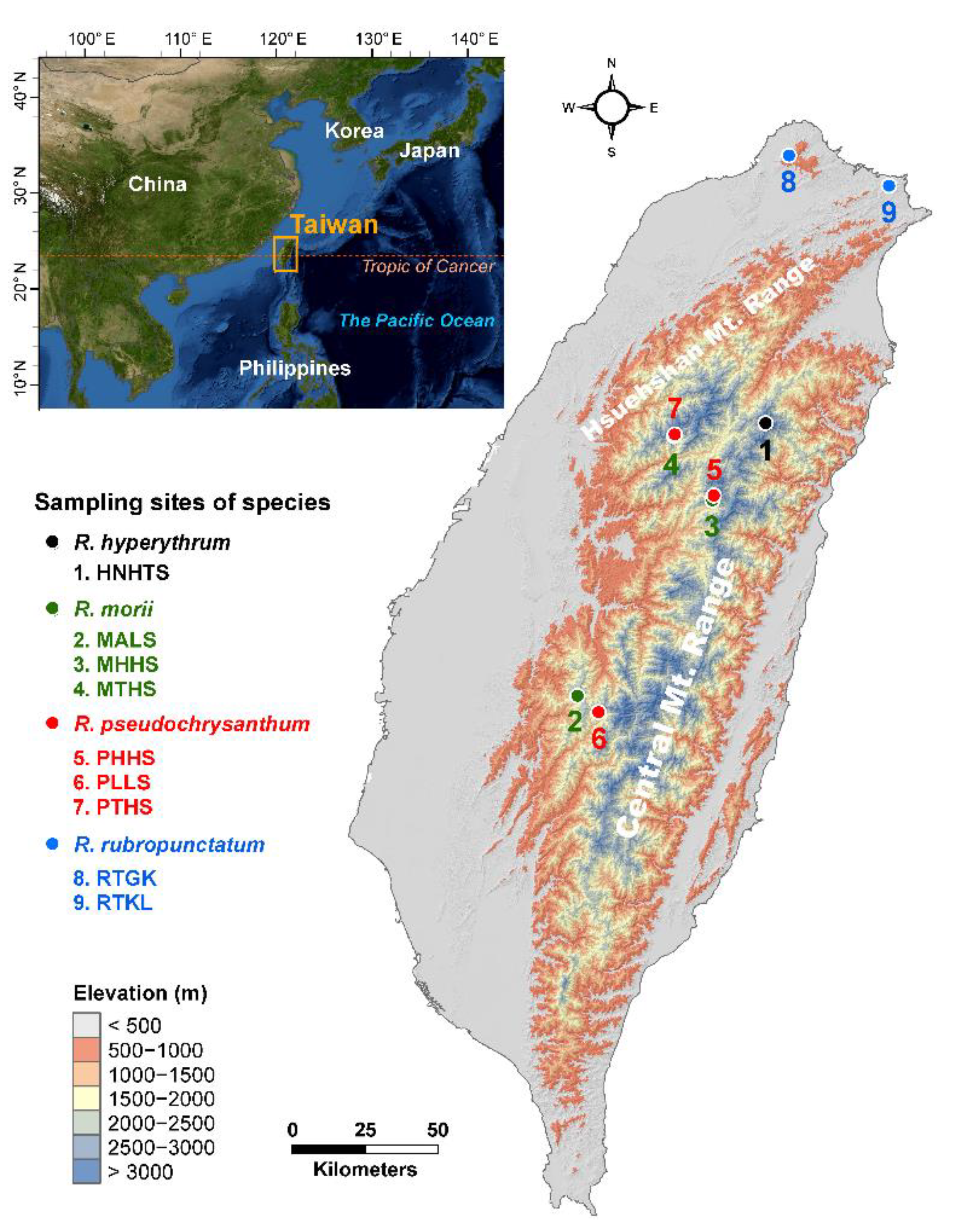
The Rhododendron pseudochrysanthum complex comprises four closely related species, including R. hyperythrum, R. morii, R. pseudochrysanthum, and R. rubropunctatum, that belong to the subgenus Hymenanthes [25]. At elevations above 3000 m, R. pseudochrysanthum grows on the periphery of cold adapted coniferous forests. R. morii inhabits the periphery of warm-temperate evergreen broadleaved forests at elevations around 2400–3000 m in central and southern Taiwan. Populations of these two species overlap at elevations of approximately 3000 m in the mountains of Hohuanshan and Tahsueshan in central Taiwan [25]. R. hyperythrum is found dominating the alpine tundra at an elevation of around 3500 m on the peak of Nanhutashan in central Taiwan. R. rubropunctatum is distributed in the northern subtropical evergreen broadleaved forests at elevations around 600–1200 m [25].
Close phylogenetic relationships were observed between the species of the R. pseudochrysanthum complex based on chloroplast DNA (cpDNA) sequences [26]. Populations of this species complex experienced north-to-south expansions during the last glacial maximum (LGM) [26]. Effective population size reductions of high-elevation Hohuanshan and Tahsueshan populations were found [10], based on the expressed sequence tag simple sequence repeats (EST-SSRs) data, indicating past range retractions because of the upward range shifts to higher elevations [5,6,7]. The current distributions of species in the R. pseudochrysanthum complex are the outcome of the past upward migration of R. hyperythrum, R. morii, and R. pseudochrysanthum populations to high elevations and the restriction of R. rubropunctatum populations in northern lower elevations. Only one out of the 26 EST-SSR loci assessed was found to be an environmentally-dependent selective outlier in global comparison and was also in pair population comparisons involving the low-elevation R. rubropunctatum populations [10]. Although the chance of potential advantageous mutations may be reduced if the effective population size decreases [1,2,3,4,5,13], population adaptive divergence found in species with low effective population size is not uncommon, particularly when selection is strong [2,3,13,14].
Tree species may diverge ecologically and lead to reproductive isolation because of divergent environments [1,2,3]. Selection can create a pattern of isolation-by-environment (IBE) [27,28] in contrast to gene flow between populations impeded solely by geographic distance (isolation-by-distance, IBD). Closely related species can be in various stages of divergence, before complete reproductive isolation is invoked by environmental differences [1]. The detection of adaptive divergence in the elevational trailing- and leading-edge populations is probable in the R. pseudochrysanthum complex, due to its demographic history of glacial expansion and postglacial upward shifting, using a large number of molecular markers. Here, 171 and 132 samples from nine and six populations of the R. pseudochrysanthum complex were surveyed for AFLP and MSAP variation, respectively. The genetic and epigenetic variations surveyed were used to test the hypothesis of the early stage ecological speciation in the R. pseudochrysanthum complex.
The AFLP and MSAP variations surveyed were used in a combination of phylogenetic; genetic clustering; genetic differentiation; genome scans; and multivariate analytic techniques to answer four specific questions: (1) Is there species integrity in the four closely related species of the R. pseudochrysanthum complex? (2) Are AFLP and MSAP FST outliers; detected by genome scans methods; associated strongly with environmental variables? (3) Does IBE play a stronger role than IBD in explaining outlier genetic and epigenetic variations? And (4) What are the most important environmental variables contributing to outlier genetic and epigenetic variations? Answering these questions will provide information to investigate the probable evolutionary process shaping the patterns of genetic diversity and phylogenetic relationships and a probability of ecological speciation of four closely related species in the R. pseudochrysanthum complex.
2. Results
2.1. Genetic Diversity Based on the Total AFLP Variation
With 171 individuals of the R. pseudochrysanthum complex (Table 1, Figure 1), eight primer combinations generated a total of 384 AFLP loci with an overall repeatability of 96.2% (Table S1). The proportion of polymorphic loci ranged from 56.0% (population PTHS) to 69.8% (population PLLS) with an average of 62.0% (Table 1). The average level of unbiased expected heterozygosity (uHE) was 0.2211 and ranged from 0.2038 (population PTHS) to 0.2439 (population RTGK). The analysis with the linear mixed effect model (LMM) showed no overall uHE significant difference when compared between species (Wald χ2 = 4.4342, p = 0.2182). Only the population pair between PLLS and PTHS had a significant uHE difference after Tukey’s p value adjustment (t = −2.637, p = 0.0085; Table S2), albeit an overall significant difference was revealed (Wald χ2 = 21.241, p = 0.0065). The test for multilocus linkage disequilibrium revealed a significant departure from random associations in both the index of association (IA) and the modified index of association (rD) between AFLP loci (Table 1).

Table 1.
Site properties and genetic parameters of sampled populations of the Rhododendron pseudochrysanthum complex estimated based on the total AFLP variation.

Figure 1.
Geographic distribution of the nine populations of four closely related species in the Rhododendron pseudochrysanthum complex occurring in Taiwan. The countries’ boundary (polygon) map was derived from the default map database in ArcGIS v.10.3 (Supplementary Methods). The elevation gradients of Taiwan (background) were presented in ArcGIS based on the 20 m digital elevation model. The locations of the sampling sites were plotted using Tools in ArcGIS by their coordinates. See Table 1 for abbreviations of the nine populations of the R. pseudochrysanthum complex.
2.2. Environmental Heterogeneity
Overall environmental heterogeneity between the sampling sites was found using permutational multivariate analysis of variance (PERMANOVA), based on the 11 retained environmental variables (Supplementary Methods, Table S3) (p = 0.001). These environmental variables include: bioclimatic (BIO1, annual mean temperature; BIO2, mean of the difference of the monthly maximum and minimum temperatures; and BIO12, annual precipitation); topographic (aspect, elevation, and slope); and ecological (CLO, cloud cover; NDVI, normalized difference vegetation index; PET, annual total potential evapotranspiration; RH, relative humidity; and WSmean, mean wind speed) variables. When compared between sample sites of different species, either significant or non-significant environmental differences can be found (Table S4). However, no significant environmental difference was found when comparing between the sample sites of the same species.
2.3. Genetic Relationships and Clustering Based on the Total AFLP Variation
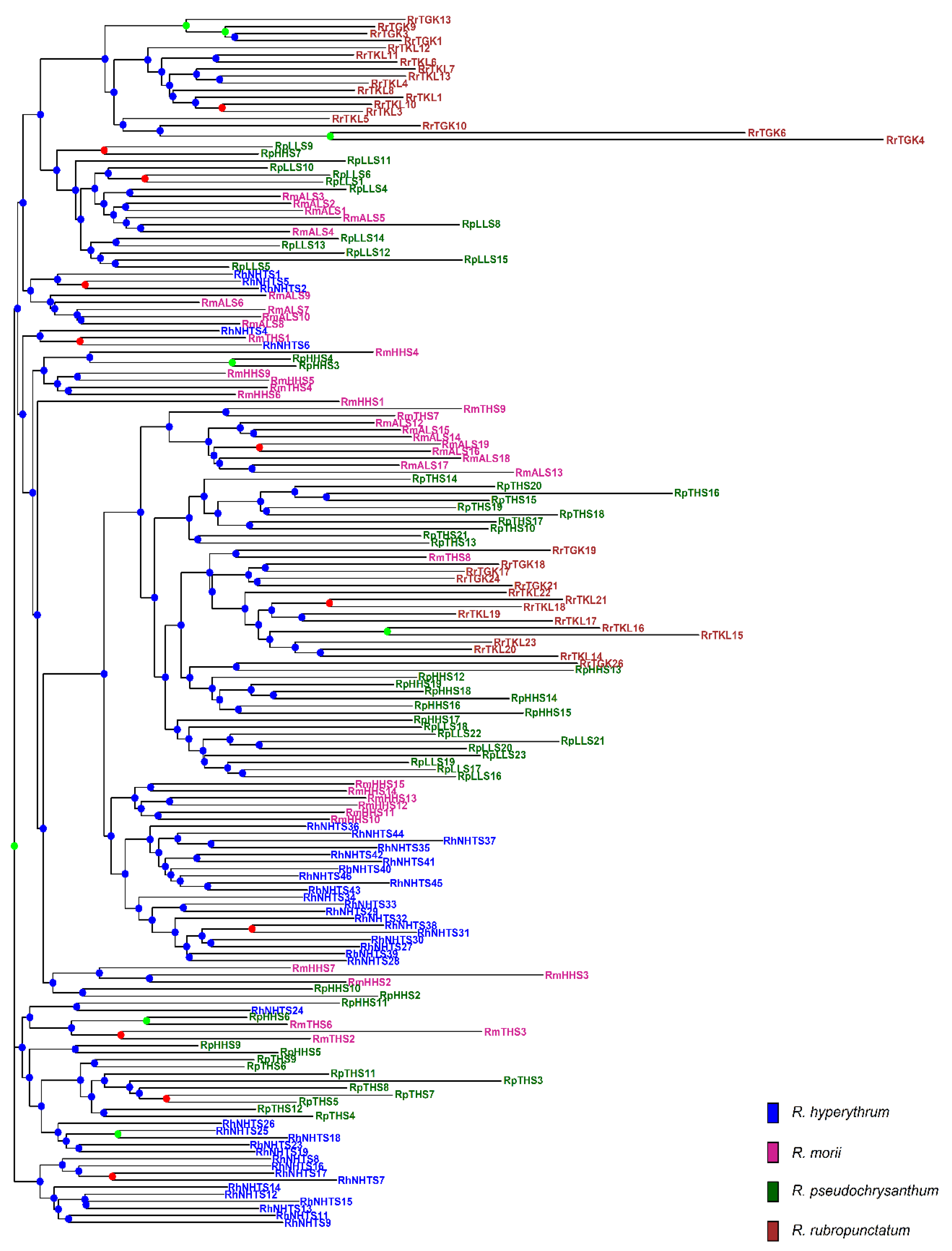
The analysis of molecular variance (AMOVA) revealed shallow, but significant species differentiation (ΦCT = 0.0520, p = 0.012; Table 2) based on the total AFLP data. The level of genetic differentiation between populations within species was significant (ΦSC = 0.1000, p = 0.001). A significantly moderate level of differentiation between populations of the R. pseudochrysanthum complex was found (ΦST = 0.1468, p = 0.001; FST = 0.0763, p < 0.001). Moderate levels of genetic differentiation (FST) were also found to be significant for all pairwise population comparisons (Table S5). Using the total AFLP data, the mean of the minimal cross entropy (CE) was minimized at K = 6 (Figure S1a) and the lowest Bayesian information criterion (BIC) was found at K = 5 (Figure S1b), respectively, using the sNMF algorithm of landscape and ecological association (LEA) [29] and the discriminant analysis of principal component (DAPC) [30,31]. Distinct population classification cannot be found, due to the high degree of shared polymorphism between individuals of different populations, as was revealed by LEA (Figure 2a). Using DAPC, three population clusters can be distinguished (Figure 2b). DAPC cluster 1 contains the two low-elevation populations RTGK and RTKL of R. rubropunctatum. DAPC cluster 2 contains individuals of populations MALS, PHHS, and PLLS, which belong to R. morii and R. pseudochrysanthum. DAPC cluster 3 included individuals of populations HNHTS, MTHS, and PTHS, which belong to R. hyperythrum, R. morii, and R. pseudochrysanthum. Nonetheless, individuals of populations HNHTS, PHHS, PTHS, and PLLS agglomerated in the periphery of clusters 2 and 3. The individual neighbor-joining (NJ) tree, generated based on the total AFLP data, with mostly low bootstrap values, revealed no distinctive relationships of individuals between populations and between species (Figure 3). Additionally, the center of the neighbor-net (NN) tree [32] was deeply intertwined and netted, which is supportive of no clear population and species distinction in the R. pseudochrysanthum complex (Figure S2). These results indicate the intermingling of individuals between populations of different species located in different geographic areas.
Table 2.
Genetic differentiation between species, between populations within species, and between nine populations of the Rhododendron pseudochrysanthum complex based on the total and outlier AFLP variation using analysis of molecular variance (AMOVA).

Figure 2.
Analysis of genetic homogeneous groups of 171 individuals from nine populations of four closely related species in the Rhododendron pseudochrysanthum complex based on the total AFLP variation using (a) LEA and (b) DAPC. The clustering scenarios for K = 2–4 were displayed in LEA. LEA, landscape and ecological association [29]; DAPC, discriminant analysis of principal component [30,31].
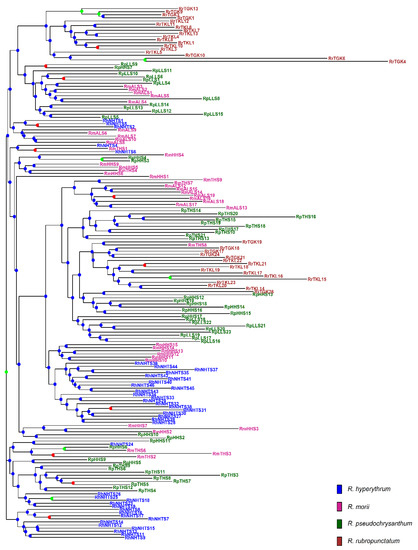
Figure 3.
The neighbor-joining (NJ) tree of 171 individuals of four closely related species in the Rhododendron pseudochrysanthum complex based on the total AFLP variation. The NJ tree was generated based on Nei’s genetic distances [33] and 1000 bootstrap replicates were used in calculating bootstrap support values. Tip labels for individuals are colored: R. hyperythrum (blue), R. morii (violet red), R. pseudochrysanthum (dark green), and R. rubropunctatum (brown). For each node, bootstrap support values greater than 70%, between 50% and 70%, and smaller than 50% were coded with green, red, and blue circles, respectively.
2.4. Potential Genetic and Epigenetic Outliers Associated with Environmental Variables and the Most Important Environmental Variables Explaining Outlier Variation
Out of 384 AFLP, 580 MSAP-m (methylated), and 274 MSAP-u (unmethylated) loci (Supplementary Methods, Table S6), 16 (4.2%), 4 (0.7%), and 15 (5.5%) loci, respectively, showed evidence of being FST outliers for population differentiation using both BAYESCAN [34] and DFDIST [35] in global comparisons (). The AFLP and MSAP primer pairs for amplification of these 35 outliers and the amplified length (bp) were listed in Table S7. These 35 loci were found to be associated with various environmental variables using LFMM (Latent factor mixed model) [36], Samβada [37], and a Bayesian logistic regression (brm) [38,39]. High levels of genetic differentiation at different hierarchical structures were found with ΦCT = 0.2283 (p = 0.011), ΦSC = 0.3099 (p = 0.001), ΦST = 0.4675 (p = 0.001) (Table 2), and among population FST = 0.2929 (p < 0.001), based on the variation of the 16 outlier AFLP loci.
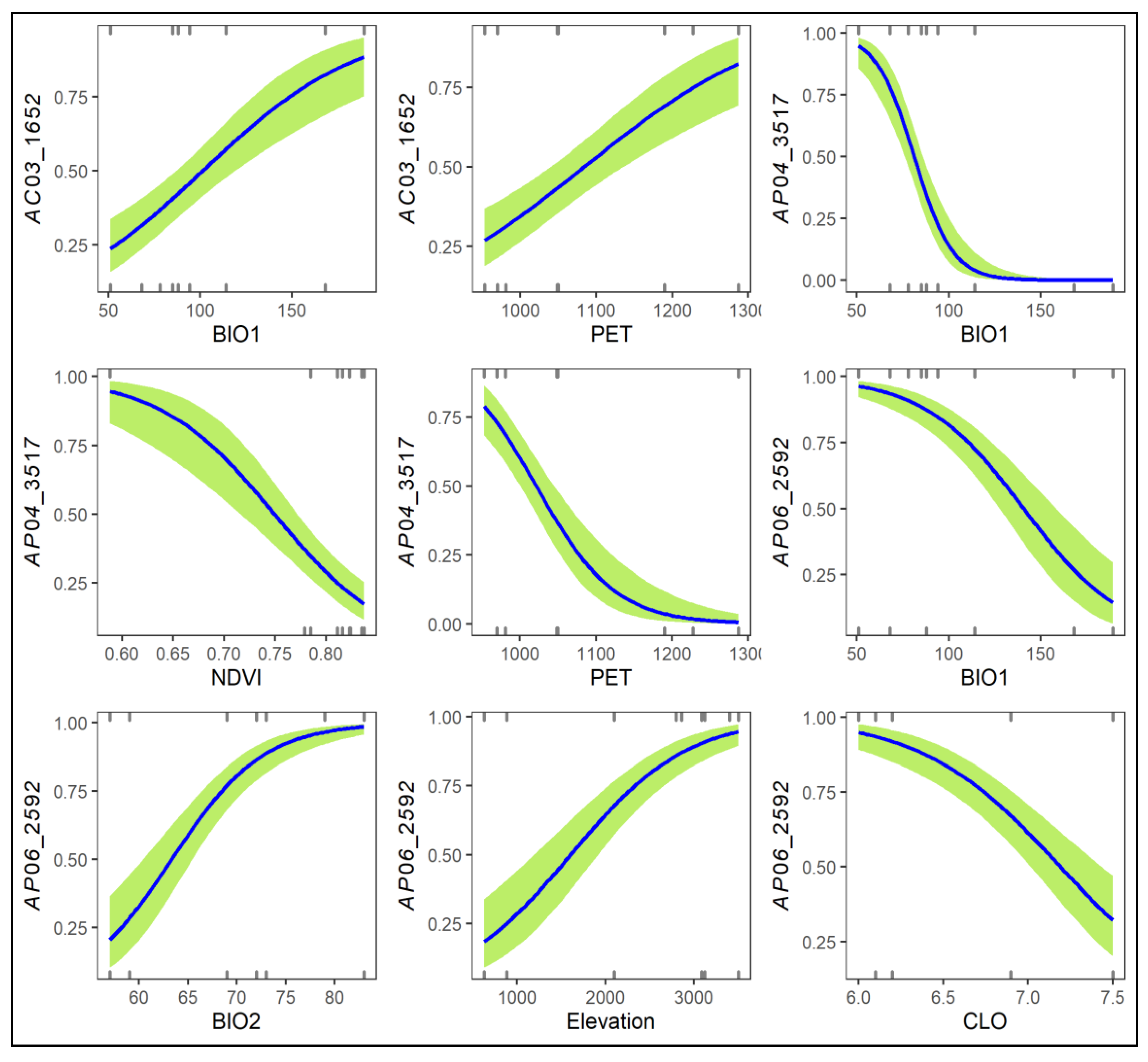
Three AFLP loci, including AC03_1652, AP04_3517, and AP06_2592, were detected as FST outliers and associated with environmental variables when compared between low-elevation trailing-edge R. rubropunctatum populations with high-elevation leading-edge populations of R. hyperythrum, R. morii, and R. pseudochrysanthum (Table S6). AC03_1652 was the potential selective outlier when compared between the RTKL population of R. rubropunctatum (high allele frequency) and populations MHHS and MTHS of R. morii (low allele frequencies) (Table S6, Figure S3). AP04_3517 was the selective outlier in comparison of the R. hyperythrum HNHTS population (high allele frequency) with both R. rubropunctatum populations (RTGK and RTKL; low allele frequencies). AP06_2592 was found to be the selective outlier when comparing R. pseudochrysanthum populations PHHS and PLLS (high allele frequencies) to the R. rubropunctatum RTGK population (low allele frequency). AC03_1652 was strongly correlated with BIO1 and PET. AP04_3517 was significantly correlated with BIO1, NDVI, and PET. AP06_2592 was found to be strongly correlated with BIO1, BIO2, elevation, and CLO. The probability estimates of these three AFLP outlier loci against the associated environmental gradients were depicted in Figure 4. Low allele frequencies in low-elevation trailing-edge populations in contrast to high allele frequencies in high-elevation leading-edge populations were found for AFLP outliers such as AC05_1828, AC05_2733, and AP06_3422 (Table S6, Figure S3). However, these loci were not detected as FST outliers by either DFDIST or BAYESCAN in pair population comparisons (Table S6).
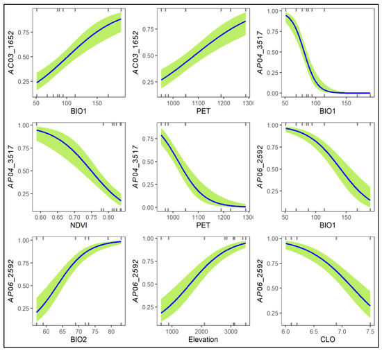
Figure 4.
Logistic regression plots of the three AFLP loci associated strongly with environmental variables when comparing the low-elevation Rhododendron rubropunctatum populations with the high-elevation populations of species including R. hyperythrum, R. morii, and R. pseudochrysanthum. Values of the y-axis are the predicted probabilities of AFLP loci and the number of the x-axis are the values of environmental variables. Logistic regression was performed based on the generalized linear model with a logit link function and a binomial residual distribution. The presence/absence of the three loci (AC03_1652, AP04_3517, and AP06_2592) were used as response variables and the environmental variables strongly correlated with the loci were used as predictor variables in analysis using the glm function of R (Supplementary Methods). BIO1, annual mean temperature; BIO2, mean of the difference of the monthly maximum and minimum temperatures; CLO, cloud cover; NDVI, normalized difference vegetation index, PET, annual total potential evapotranspiration.
No apparent contrasting differences in allele frequencies comparing the trailing- and leading-edge populations were found in all 15 outlier MSAP-u loci. Although a higher MSAP-m MP5_1240 allele frequency in the low-elevation trailing-edge population (RTKL) was found in contrast to high-elevation leading-edge populations with lower allele frequencies, no MSAP locus was detected as FST outlier by either BAYESCAN or DFDIST when comparing low-elevation trailing-edge populations to high-elevation leading-edge populations (Table S6).
Eleven environmental variables, including three bioclimatic (BIO1, BIO2, and BIO12), three topographic (aspect, elevation, and slope), and five ecological (CLO, NDVI, PET, RH, and WSmean) variables (Table S3), were used separately for forward selection analysis [40] to assess their contributions in explaining outlier AFLP variation. For the investigation of the contributions of environmental variables in explaining outlier MSAP variation, ecological variables CLO and WSmean were removed due to collinearity with the other three ecological variables in the six populations examined for MSAP. The most important environmental variables in the three environmental categories were BIO1 (adjusted R2 = 0.1576), elevation (adjusted R2 = 0.1394), and PET (adjusted R2 = 0.1150), respectively, explaining the outlier AFLP variation (Table 3). The most important environmental variables in the three environmental categories were BIO1 (adjusted R2 = 0.1925), elevation (adjusted R2 = 0.1272), and PET (adjusted R2 = 0.1664), respectively, explaining the outlier MSAP-m variation. BIO1 (adjusted R2 = 0.3446), elevation (adjusted R2 = 0.1772), and NDVI (adjusted R2 = 0.3518) were the most important environmental variables in the three environmental categories, respectively, explaining the outlier MSAP-u variation.
Table 3.
Relative contribution (adjusted R2) and F test of environmental variables explaining outlier genetic and epigenetic variations of the Rhododendron pseudochrysanthum complex using a forward selection procedure.
2.5. Relative Contribution of IBD and IBE Explaining Outlier Genetic and Epigenetic Variations
The retained 11 and 9 environmental variables were used in testing for IBD and IBE, respectively, based on the total variation. Significant relationships between environmental and geographic distances were found using a Mantel test and multiple matrix randomization regression (MMRR) [41] (Table 4). Except for the MSAP-m data, significant IBD was found in all the analyses based on the total variation using a Mantel test and MMRR. Partial Mantel tests found significant IBE based on the total AFLP and MSAP-u variations. A significant adaptive divergence can be inferred based on the three outlier datasets, controlling for geography using the partial Mantel test (AFLP: Mantel r = 0.2858, p = 0.001; MSAP-m: Mantel r = 0.1551, p = 0.001; MSAP-u: Mantel r = 0.0825, p = 0.002).
Table 4.
Isolation-by-environment and isolation-by-distance tested using Mantel test, partial Mantel tests, and multiple matrix regression with randomization (MMRR). Euclidean distance matrices were generated based on AFLP, MSAP-m, and MSAP-u (G), geography (D), and environment (E). MMRR was used to infer the effects of geographic (βD) and environmental (βE) distances on genetic (AFLP) and epigenetic (MSAP-m and MSAP-u) distances. R2 represents the total amount of variation explained by both geographic and environmental factors. When outlier datasets were used, strong adaptive divergence can be inferred if significance was found controlling for geographic effect.
MMRR implements a combined model of geographic and environmental distances, which revealed patterns of significant IBE based on the total data. MMRR showed that environmental and geographic factors together explained 19.02% AFLP, 0.46% MSAP-m, and 5.09% MSAP-u variation of the total data; and 28.97% AFLP, 10.74% MSAP-m, and 4.93% MSAP-u variation of the outlier data. Additionally, MMRR revealed genetic and epigenetic adaptive divergences strongly correlated with environments based on the outlier datasets (AFLP: βE= 0.3074, p = 0.001 vs. βD = 0.2488, p = 0.001; MSAP-m: βE = 0.3412, p = 0.001 vs. βD = −0.0175, p = 0.5755; MSAP-u: βE = 0.3431, p = 0.001 vs. βD = −0.1351, p = 0.001; Table 4).
3. Discussion
Genetic diversity in natural plant populations can be shaped by the mating system, pollen and seed dispersal, life form, past incidents such as range expansions, bottlenecks or founder events, and natural selection [7,10,20,26]. The levels of AFLP diversity were also found to be lower in the four species of the R. pseudochrysanthum complex compared with other Rhododendron species, including R. calophytum, R. purdomii, R. concinnum, R. clementinae, and R. capitatum [42]. However, the levels of AFLP diversity in the species of the R. pseudochrysanthum complex were similar to a narrowly distributed endangered species, Rhododendron protistum var. giganteum [43]. The species level AFLP diversity in the R. pseudochrysanthum complex was also similar to the average AFLP diversity summarized for 13 plant species [19]. Maintaining intraspecific genetic diversity is critical for a species to adapt and crucial to short-term and long-term survival [2,3,44]. Outcrossing is the predominant mating system in Rhododendron [45,46,47] and is thought to enhance the level of population genetic diversity; however, the relatively lower levels of population genetic diversity in species of the R. pseudochrysanthum complex might have resulted from past evolutionary history, such as population retractions due to postglacial upward shifting [10]. Since the LGM, a 1500 to 1600 m upward migration of forests was reported [48] and the population sizes of tree species, such as Rhododendron, in Taiwan are expected to decrease [7,10]. Range reductions can have significant genetic and evolutionary impacts, resulting in the loss of genetic diversity and consequences for population survival, and detrimental effects may have a marked influence on the distribution of marginal populations [49,50].
Although gene flow plays a critical role in shaping the current population genetic structure, the degree of gene flow estimated empirically may also reflect the population demographic history [51]. The DAPC clustering results demonstrated the apparent distinction of individuals of R. rubropunctatum from individuals of other species in the R. pseudochrysanthum complex (Figure 2b), but such inference cannot be made based on the results of LEA (Figure 2a), the NJ tree (Figure 3), and the NN tree (Figure S2). These results suggest that the four closely related species in the R. pseudochrysanthum complex can be combined into a single species [52] and are consistent with the results obtained based on cpDNA [26] and nuclear internal transcribed spacer sequences [53].
The pattern of relatively homogeneous levels of genetic diversity (Table S2) can be expected under an incomplete lineage sorting scenario [54]. The omnipresence of the intermingling of individuals between populations and between species, indicated by both NJ and NN trees (Figure 3, Figure S2), suggests short divergence times between taxa with historical large population sizes and/or the retention of ancestral polymorphism [10,26]. Nonetheless, these results may also be caused by the hybridization within the R. pseudochrysanthum complex, in which individuals of different populations and different species are grouped into the same clades. The predominant insect pollination in Rhododendron [55,56] and the tiny, winged seeds produced are likely to be dispersed by wind over a distance of approximately 30–80 m [56,57]; long distance recurrent gene flow leading to hybridization among individuals of different populations of the R. pseudochrysanthum complex is less likely. However, historical migration cannot be excluded [10,26]. The hypothesis predicts a positive correlation between the pairwise population spatial distance and population genetic differentiation due to limited gene flow, and historical gene flow can be inferred by regressing the pairwise population differentiation on geographic distance [54]. In the present study, historical gene flow can be inferred because of the significant correlations of pairwise FST (estimated based on the total AFLP) with Euclidean distances between the sample sites, calculated based on geographic coordinates, which were were found using Spearman’s rank correlation test (ρ = 0.669, S = 2570, p < 0.0001; Figure S4).
There are more than 200 peaks exceeding 3000 m in elevation with varied geographic topographies in mountainous regions in Taiwan. Because gravity is a crucial factor in seed dispersal [47,56], the contemporary seed dispersal of Rhododendron might be even more limited, considering that elevational differences and mountain ranges can be effective barriers to genetic exchange [58] in the distribution range of this species complex. Moreover, the general significant IBD pattern suggests a dispersal limitation at the spatial scale, which was assessed using a Mantel test and MMRR (Table 4). However, the current gene flow between species distributed in close proximity is probable, particularly in the case of R. pseudochrysanthum and R. morii, because their flowering times overlap, with the later flowers during March to May and the former flowers during April to June. Overlapping flowering times can result in a low level of genetic differentiation such as between population MHHS and population PTHS (FST = 0.0660), which are distributed in Hohuanshan (Table S5).
Environmental differences due to landscape heterogeneity in various deep valleys and high peaks of mountainous regions in Taiwan may play a role in limiting rather than promoting Rhododendron dispersal, and IBE would be relatively pronounced in contrast to IBD. Strong IBE indicates habitat isolation or immigrant inviability and may lead to reproductive isolation due to local environmental conditions, resulting in the reduced survival and reproduction of migrants [27,28]. We combined the use of one measure of environmental distance matrix generated from multiple environmental variables and an individual-based approach [59]; strong adaptive divergence was found, using a partial Mantel test and MMRR regression analysis, based on the outlier datasets (Table 4). Because geography and environment are not mutually exclusive in influencing genetic variation, both IBD and IBE can be effective in restricting gene flow between populations via direct and indirect processes [17,20,27,28,41]. Our results showed strong adaptive divergence using both the partial Mantel test and MMRR based on the outlier AFLP and MSAP datasets, suggesting that adaptive evolution caused by environmental differences may be important to the on-going and future process of ecological speciation in the R. pseudochrysanthum complex.
Three outlier loci (AC03_1652, AP04_3517, and AP06_2592) were found by pairwise comparisons between the leading- and trailing-edge populations, with high or low allele frequencies, indicating an adaptation associated with local environments. Increases in the levels of genetic divergence and the rate of speciation are, among others, found to be closely associated with temperature [60,61]. Temperature shifts have been found to play prominent roles in driving adaptive genetic and epigenetic variations in various plant species [10,17,20,23,24,62,63]. Our results suggest that temperature was the most important bioclimatic factor, with a high adjusted R2 value (Table 3), explaining the genetic and epigenetic variations among populations of the R. pseudochrysanthum complex. PET is a measure that accounts for water loss via transpiration [64] and was found to be the most important ecological factor (Table 3) highly associated with adaptive AFLP and MSAP-m variations (Table S6). PET was found to be associated with adaptive genetic variation in Picea glauca [65] and may be related to the increase in the adaptive capacity of trees under global warming in a drying climate. PET-related drought stress has also been found to be associated with epigenetic variation in Vicia faba [66]. Genetic differences between Saccharum species [67] and between populations of Populus angustifolia [68] were found to be related to the difference in traits that have the ability to maintain a favorable water balance. NDVI is a measure of surface coverage activity, representing the degree of vegetation greenness, suggestive of a biotic competitive environment that might play a role in interactions with other species in a local ecological community [69,70]. NDVI has been shown to be correlated with epigenetic variation in a coniferous species, Taiwania cryptomerioides [71]. The measurement of NDVI can range from −1 to 1, and a higher NDVI value indicates greater plant health [72]. The habitat of R. hyperythrum had a relatively lower NDVI value compared with that of other populations of the R. pseudochrysanthum complex (Table S3). The R. hyperythrum population at a high elevation might have evolved a local adaptation because of a selective outlier (AP04_3517) (Table S6) with a very high allele frequency in contrast to the extremely low allele frequencies of low-elevation populations (Figure S3). However, the habitat of the R. hyperythrum population with a low NDVI value suggests that it may be under threat of high elevation environments (e.g., a high UV condition).
Elevation is the most important topographic factor explaining outlier genetic and epigenetic variations (Table 3). Environmental variables can be classified into those highly correlated with altitude, such as annual mean temperature (r = −0.973), and those with a lower correlation coefficient, such as PET (r = −0.668) and NDVI (r = −0.420) in this study [73], which could have played roles in driving the population adaptive genetic and epigenetic divergences in the R. pseudochrysanthum complex. The elevational difference in meters is not a factor driving population divergence and may not be a useful predictor for distribution modeling [74]. However, elevation-dependent environmental conditions can be complex [75] and altitude-associated abiotic conditions may play important roles in shaping non-random variations of outlier allele frequencies and resulting in spatially-structured intraspecific genetic and epigenetic variations [10,24,76,77]. It is interesting that we found a higher probability estimate of an outlier AFLP locus (AP06_2592) with high allele frequencies at high-elevation populations (Figure 4). This locus was found to be significantly positively or negatively correlated with the environmental variables examined, such as annual mean temperature, mean of the difference of the monthly maximum and minimum temperatures, and cloud cover (Figure 4, Table S6, Figure S3). Additionally, elevational differences explaining outlier genetic and epigenetic variations may not only represent those abiotic factors examined in this study but also those that are not examined [78].
4. Materials and Methods
4.1. Sampling, Genotyping, and Epigenotyping
We collected fresh leaf samples of 171 individuals from nine populations of the R. pseudochrysanthum complex (Table 1, Figure 1) and used them for total DNA extraction [79] (Supplementary Methods). We surveyed the genetic variation of 171 individuals from nine populations using AFLP (Table 1). Due to a technical problem, 132 individuals from six populations were used in epigenotyping using MSAP. In AFLP, a total of 10 µL reaction volume, containing 6 µL (200 ng) of total genomic DNA digested with 0.5 µL EcoRI (20 UµL−1) and mixed with 1 µL MseI (10 UµL−1), 1.5 µL ddH2O, and 1 µL CutSmart buffer (New England Biolabs, Ipswich, MA, USA), was incubated at 37 °C for 1.5 h. The reaction was terminated at 65 °C for 15 min. The digested DNA products were ligated with 1 µL (5 µM) of the EcoRI adaptor and 1 µL (50 µM) of the MseI adaptor using 1 µL (5 UµL−1) T4 DNA ligase (Thermo Scientific, Vilnius, Lithuania), 3 µL ddH2O, and 4 µL 5X ligation buffer (Thermo Scientific, Vilnius, Lithuania) in a 10 µL ligation reaction mixture at 22 °C for 1 h.
Pre-selective amplification was performed using 4 µL diluted digested samples (1:9 dilution with ddH2O) as a template in a 20 µL volume containing 8.6 µL ddH2O, 2 µL 10X PCR buffer (Zymeset Biotech, Taipei, Taiwan), 1.6 µL EcoRI (16 µM; E00: 5′-GACTGCGTACCAATTC-3′), 1.6 µL MseI (16 µM; M00: 5′-GATGAGTCCTGAGTAA-3′) primers, 1.6 µL dNTPs (2.5 mM), 0.4 µL MgCl2 (0.15 mM), and 0.2 µL Taq DNA polymerase (5 UµL−1; Zymeset). The pre-selective amplification was performed with an initial holding at 72 °C for 2 min and pre-denaturation at 94 °C for 3 min, followed by 25 cycles of 30 s at 94 °C, 30 s at 56 °C, and 1 min at 72 °C, with a final 5 min holding at 72 °C. Eight EcoRI-MseI (E00 and M00) selective primer combinations with additional bases added at the ends were used for AFLP selective amplification (Table S1). EcoRI selective primer was labeled with fluorescent dye (6-carboxyfluorescein or hexachloro-fluorescein) and amplification was performed in a 20 µL volume containing 11.3 µL ddH2O, 2 µL 10X PCR buffer (Zymeset), 2 µL EcoRI (20 µM), 2 µL MseI (20 µM) primers, 1.6 µL dNTPs (2.5 mM), 0.1 µL Taq DNA polymerase (5 UµL−1; Zymeset), and 1 µL diluted pre-selective amplified product (1:19 dilution with ddH2O). We performed selective amplification with an initial holding at 94°C for 3 min, followed by 13 cycles of 30 s at 94 °C, 30 s at 65–56 °C (decreasing the temperature by 0.7 °C each cycle), 1 min at 72 °C, then 23 cycles of 30 s at 94 °C, 30 s at 56 °C, and 1 min at 72 °C, with a final 5 min holding at 72 °C. In MSAP, the AFLP protocol was adapted by replacing restriction enzyme MseI with the methylation-sensitive enzymes HpaII and MspI in two separate experiments. Ten MSAP selective primer combinations were used with additional nucleotides at the ends of the E00 and HM00 (HpaII-MspI, 5′-ATCATGAGTCCTGCTCGG-3′) (Table S1).
PCR amplification products were electrophoresed on an ABI 3730XL DNA analyzer and scored with Peak Scanner v.1.0 (Applied Biosystem, Foster City, CA, USA). We scored AFLP and MSAP fragments using a fluorescent threshold set at 150 units in the range of 100–500 bp. The “mixed scoring 1” of the MSAP-calc R script [80] in the R environment [81] was used to transform MSAP markers to two distinct types of data: MSAP-m (methylated) and MSAP-u (unmethylated) datasets [82]. Error rate per locus for AFLP and MSAP were calculated (Supplementary Methods, Table S1). Loci with an error rate per locus greater than 5% were removed [83].
4.2. Genetic Diversity Based on the Total AFLP Variation
The proportion of polymorphic loci and uHE [84,85] were estimated using AFLP-SURV v.1.0 [86]. uHE per locus was estimated using ARLEQUIN v.6.0 [87]. To test departure from linkage equilibrium indicating a possibility of inbreeding or non-random associations between alleles, measures of multilocus linkage disequilibrium, including IA [88] and rD [89], were estimated using the ia function of R poppr package [90] with 999 permutations. LMM, considering population as a fixed factor and locus as a random factor, was used to test the difference of mean uHE per locus among species and among populations using the lmer function of R lme4 package [91], and significance was tested using the Anova function of R car package based on type II Wald χ2 statistic [92]. Tukey’s multiple comparison test was applied for pairwise species and pairwise population comparisons using the lsmeans function of R emmeans package [93].
4.3. Environmental Heterogeneity
A Pearson’s correlation coefficient threshold of |0.8| between environmental variables (Supplementary Methods) was used to calculate variance inflation factor (VIF) separately for variables within each environmental category (bioclimate, ecology, and topography) (Supplementary Methods) using the vifcor function of R package usdm [94]. VIF values greater than 5 within each environmental category were removed. Pearson’s correlation coefficients of pairwise comparisons between variables were calculated and depicted in Figure S5. Environmental differences among species and among sample sites were assessed using PERMANOVA implemented in the adonis function of R package vegan [95], and pairwise comparisons assessed using the pairwise.perm.manova function of R package RVAideMemoire [96] with 999 permutations and a 5% false discovery rate (FDR).
4.4. AFLP Genetic Clustering and Relationships
Genetic homogeneous groups of individuals were assessed using sNMF algorithm [29] and DAPC [30] (Supplementary Methods). Individual assignments with K = 1–9 based on least-squares optimization using the snmf function of R LEA package [29]. The find.clusters and dapc functions of R adegenet package [31] were used in DAPC analysis. Genetic relationships among individuals were assessed using NJ and NN trees. The NJ tree was generated based on Nei’s genetic distances [33] using the nei.dist functions of R poppr package and the nj function of R package ape [97]. The NN tree was generated using the neighborNet function of R package phangorn [98]. The bootstrap values were calculated using 1000 bootstrap replicates with the aboot function of R package poppr for both NJ and NN trees.
4.5. Test for AFLP and MSAP FST Outliers
BAYESCAN and DFDIST were used to identify FST outliers (Supplementary Methods). BAYESCAN v.2.1 [34] was used to estimate the ratio of posterior probabilities of selection over neutrality (the posterior odds (PO)). A logarithmic scale of log10PO > 0.5 was defined as substantial evidence for selection over neutrality in BAYESCAN [99,100] (Supplementary Methods). DFDIST was used to estimate a distribution of observed FST versus uHE, and loci falling above the 95% confidence level of simulated distribution were identified as potential FST outliers. Global and pairwise population comparisons were performed in BAYESCAN and DFDIST.
4.6. AFLP Genetic Differentiation
AMOVA was used to estimate the hierarchical level of genetic differentiation using the poppr.amova function of R package poppr, and significance was tested using the randtest function of R package ade4 [101] with 9999 permutations. Both the total and outlier AFLP data were used in AMOVA. Among population, FST was also estimated using AFLP-SURV. Pairwise population FST was computed using ARLEQUIN based on the total and outlier AFLP data, and significance was tested with 10,000 permutations.
4.7. Associations of Genetic and Epigenetic Loci with Environmental Variables
LFMM [36] and Samβada [37] were employed to assess the associations of all genetic and epigenetic loci with environmental variables (Supplementary Methods). In LFMM, the number of latent factors was set to 3 and Z-scores of ten independent runs were combined using Fisher–Stouffer method [102]. p values were adjusted using the genomic inflation factor (λ) and a 1% FDR. Samβada was used to evaluate the associations of allele frequencies with the values of environmental variables. Both Wald and G scores with a 1% FDR for p value adjustment were used in assessing the fit of model with environmental variables against null model without environmental variables.
Loci found to be associated strongly with environmental variables assessed using Samβada and LFMM were further tested with a Bayesian logistic regression analysis implemented in the brm function of R brms package [38,39] (Supplementary Methods). Student’s t distribution with mean zero and seven degrees of freedom were used as the weakly informative priors, and the scale of the prior distribution was 2.5 for intercept and predictors using the set_prior function. Credible intervals (95%) were determined using the posterior_summary function.
4.8. AFLP and MSAP Isolation-by-Environment and Isolation-by-Distance
The correlations of the total and outlier Euclidean distance matrices with the Euclidean distance matrix of environmental variables were analyzed in a Mantel test using the mantel function of R vegan package with 999 permutations. Partial Mantel test was performed, controlling for geographic effect (latitude and longitude) using the mantel.partial function of R vegan package. MMRR was performed using the MMRR function [27] of R. Regression coefficients of IBE or adaptive divergence (βE) and IBD (βD) were obtained and significance was determined after 999 permutations. Models for redundancy analysis generated using the rda function of R vegan package were used in the forward selection [40] to test for the most important environmental variables explaining outlier genetic and epigenetic variations by using the forward.sel function of R adespatial package [103].
5. Conclusions
Understanding the roles that geography and environment play in speciation is an important issue in evolutionary biology [1,3,27,28,60,61]. Evolutionary processes, including incomplete lineage sorting and historical migration, might have played important roles in causing an intermingling of the genealogical relationships, revealed particularly in the NJ and NN trees, among individuals of the four closely related species in the R. pseudochrysanthum complex. A single ancestral phyletic line may diverge into a series of lineages, albeit with a shallow split in individual-based phylogenetic NJ and NN trees, adapting to rather different habitats. Our sampling of populations of the R. pseudochrysanthum complex, distributed at elevations below 1000 m and above 2000 m, and up to 3500 m, spanning a wide range of annual mean temperatures (5.1–18.9 °C), NDVI indexes (0.588–0.837), and PET indexes (953.2–1227.5), contributed to outlier genetic and epigenetic variations. The relatively stronger strength of IBE than IBD suggests spatial genetic and epigenetic structures driven by environmental conditions, and a strong IBE might play critical roles in causing the reproductive isolation and ecological speciation of closely related species in the R. pseudochrysanthum complex. However, locally adapted ecological lineages may risk extinction when encountering other environmental stressors during the course of migration. R. hyperythrum that grows in alpine tundra at high elevation may be vulnerable due to the detrimental effect of high-elevation environments on the growth of this species. Additionally, the introgression of adaptive genetic and epigenetic alleles and/or their combinations [82,104], harbored in low-elevation environments, into the genetic and epigenetic backgrounds of high-elevation locales, could be important, in particular, in the assisted migration program in the face of global change [105,106].
Supplementary Materials
The following supporting information can be downloaded at: https://www.mdpi.com/article/10.3390/plants11091226/s1, Supplementary Methods; Table S1: Primer combinations, number of markers, and error rate per locus in AFLP and MSAP techniques for investigation in the Rhododendron pseudochrysanthum species complex; Table S2: Summary of Tukey’s post-hoc pairwise population comparisons of the mean unbiased expected heterozygosity (uHE) per locus using a linear mixed effect model. In linear mixed effect model, population was treated as a fixed factor and locus as a random factor based on the total AFLP variation of the Rhododendron pseudochrysanthum complex; Table S3: The 11 retained site environmental variables of the nine populations of the Rhododendron pseudochrysanthum species complex. See Table 1 for abbreviations of the nine populations; Table S4: p values of pairwise population comparisons of the 11 retained environmental variables of sample site of the Rhododendron pseudochrysanthum complex using PERMANOVA; Table S5: Pairwise FST (below diagonal) and p values (above diagonal) between populations of the Rhododendron pseudochrysanthum complex based on the total and outlier AFLP data using ARLEQUIN with 10,000 permutations; Table S6: Potential genetic (AFLP) and epigenetic (MSAP-m and MSAP-u) FST outliers identified by BAYESCAN and DFDIST associated with environmental variables assessed using Samβada, LFMM, and the brm function of R brms package; Table S7: Primer combination and amplified length for the 35 outliers presented in the Table S6. See Table S1 for E00, M00, and HM00 primer sequences. Figure S1: Evaluation of clustering scenarios based on (a) minimum cross-entropy and (b) Bayesian information criterion analyzed using LEA and DAPC, respectively; Figure S2: The neighbor-net tree of 171 individuals of four closely related species in the Rhododendron pseudochrysanthum complex. Tip labels for individuals of the four closely related species are colored: R. hyperythrum (blue), R. morii (violet red), R. pseudochrysanthum (dark green), and R. rubropunctatum (brown); Figure S3: Distribution of allele frequencies of the thirty-five FST outliers associated strongly with environmental variables across the nine populations of the Rhododendron pseudochrysanthum complex; Figure S4: The relationships of population pairwise FST with Euclidean distances between sample sites. Population pairwise FST was calculated using ARLEQUIN and Euclidean distances between sample sites were calculated based on geographic coordinates using the dist function of R stats package. Significance of the relationships were tested using Spearman’s correlation test (the cor.test function of R stats package) based on the total (blue line, ρ = 0.669, S = 2570, p < 0.0001) and outlier (red line, ρ = 0.634, S = 2844, p < 0.0001) AFLP datasets. The light blue and light red shades represent 95% confidence intervals of predicted values of simple linear regression; Figure S5: Pearson’s correlation coefficients between the 11 retained environmental variables. Aspect (0–360°) and slope (0–90°). BIO1, annual mean temperature; BIO2, mean of the difference of the monthly maximum and minimum temperatures; BIO12, annual precipitation; CLO, cloud cover; NDVI, normalized difference vegetation index, PET, annual total potential evapotranspiration; RH, relative humidity; WSmean, mean wind speed. References [107,108,109,110,111,112,113,114,115,116,117,118,119,120] are cite d in the supplementary materials.
Author Contributions
S.-Y.H. proposed, funded, and designed the research; J.-D.C. and S.-Y.H. collected samples; J.-J.C. and Y.-S.L. performed research; S.-Y.H., J.-J.C., Y.-S.L., and C.-T.C. analyzed data; S.-Y.H., J.-J.C., and Y.-S.L. wrote the paper. All authors have read and agreed to the published version of the manuscript.
Funding
This work was funded by the Taiwan Ministry of Science and Technology under grant number of MOST109-2313-B-003-001-MY3 to S.Y.H.
Data Availability Statement
The data presented in this study are available on request from the corresponding author.
Acknowledgments
The authors are grateful to Ji-Shen Wu of Taiwan Forestry Research Institute for the collection of the plant materials.
Conflicts of Interest
The authors declare no conflict of interest.
References
- Schluter, D. Evidence for ecological speciation and its alternative. Science 2009, 323, 737–741. [Google Scholar] [CrossRef] [PubMed] [Green Version]
- Jump, A.S.; Marchant, R.; Peñuelas, J. Environmental change and the option value of genetic diversity. Trends Plant Sci. 2009, 14, 51–58. [Google Scholar] [CrossRef] [PubMed]
- Kawecki, T.J.; Ebert, D. Conceptual issues in local adaptation. Ecol. Lett. 2004, 7, 1225–1241. [Google Scholar] [CrossRef] [Green Version]
- Anderson, B.J.; Akçakaya, H.R.; Araújo, M.B.; Fordham, D.A.; Martinez-Meyer, E.; Thuiller, W.; Brook, B.W. Dynamics of range margins for metapopulations under climate change. Proc. R. Soc. B 2009, 276, 1415–1420. [Google Scholar] [CrossRef] [Green Version]
- Hargreaves, A.L.; Bailey, S.F.; Laird, R.A. Fitness declines towards range limits and local adaptation to climate affect dispersal evolution during climate-induced range shifts. J. Evol. Biol. 2015, 28, 1489–1501. [Google Scholar] [CrossRef]
- Lenoir, J.; Gégout, J.C.; Marquet, P.A.; de Ruffray, P.; Brisse, H.A. Significant upward shift in plant species optimum elevation during the 20th century. Science 2008, 320, 1768–1771. [Google Scholar] [CrossRef]
- Jump, A.S.; Huang, T.-J.; Chou, C.-H. Rapid altitudinal migration of mountain plants in Taiwan and its implications for high altitude biodiversity. Ecography 2012, 35, 204–210. [Google Scholar] [CrossRef]
- Ackerly, D.D. Community assembly, niche conservatism, and adaptive evolution in changing environments. Int. J. Plant Sci. 2003, 164, S165–S184. [Google Scholar] [CrossRef]
- Hampe, A.; Petit, R.J. Conserving biodiversity under climate change: The rear edge matters. Ecol. Lett. 2005, 8, 461–467. [Google Scholar] [CrossRef] [Green Version]
- Chen, C.-Y.; Liang, B.-K.; Chung, J.-D.; Chang, C.-T.; Hsieh, Y.-C.; Lin, T.-C.; Hwang, S.-Y. Demography of the upward-shifting temperate woody species of the Rhododendron pseudochrysanthum complex and ecologically relevant adaptive divergence in its trailing edge populations. Tree Genet. Genom. 2014, 10, 11–126. [Google Scholar] [CrossRef]
- Dirnböck, T.; Essl, F.; Rabitsch, W. Disproportional risk for habitat loss of high-altitude endemic species under climate change. Glob. Chang. Biol. 2011, 17, 990–996. [Google Scholar] [CrossRef]
- Bennett, S.; Duarte, C.M.; Marbà, N.; Wernberg, T. Integrating within-species variation in thermal physiology into climate change ecology. Phil. Trans. R. Soc. B 2019, 374, 20180550. [Google Scholar] [CrossRef] [Green Version]
- Leimu, R.; Fischer, M. A meta-analysis of local adaptation in plants. PLoS ONE 2008, 3, e4010. [Google Scholar] [CrossRef] [Green Version]
- Holderegger, R.; Herrmann, D.; Poncet, B.; Gugerli, F.; Thuiller, W.; Taberlet, P.; Gielly, L.; Rioux, D.; Brodbeck, S.; Aubert, S.; et al. Land ahead: Using genome scans to identify molecular markers of adaptive relevance. Plant Ecol. Div. 2008, 1, 273–283. [Google Scholar] [CrossRef]
- Richards, C.L.; Bossdorf, O.; Verhoeven, K.J. Understanding natural epigenetic variation. New Phytol. 2010, 187, 562–564. [Google Scholar] [CrossRef]
- Richards, C.L.; Alonso, C.; Becker, C.; Bossdorf, O.; Bucher, E.; Colomé-Tatché, M.; Durka, W.; Engelhardt, J.; Gaspar, B.; Gogol-Döring, A.; et al. Ecological plant epigenetics: Evidence from model and non-model species, and the way forward. Ecol. Lett. 2017, 20, 1576–1590. [Google Scholar] [CrossRef] [Green Version]
- Shih, K.-M.; Chang, C.-T.; Chung, J.-D.; Chiang, Y.-C.; Hwang, S.-Y. Adaptive genetic divergence despite significant isolation-by-distance in populations of Taiwan Cow-tail fir (Keteleeria davidiana var. formosana). Front. Plant Sci. 2018, 9, 92. [Google Scholar] [CrossRef] [Green Version]
- Vos, P.; Hogers, R.; Bleeker, M.; Reijans, M.; van der Lee, T.; Hornes, M.; Frijters, A.; Pot, J.; Peleman, J.; Kuiper, M. AFLP: A new technique for DNA fingerprinting. Nucl. Acids Res. 1995, 23, 4407–4414. [Google Scholar] [CrossRef] [Green Version]
- Nybom, H. Comparison of different nuclear DNA markers for estimating intraspecific genetic diversity in plants. Mol. Ecol. 2004, 13, 1143–1155. [Google Scholar] [CrossRef]
- Chien, W.-M.; Chang, C.-T.; Chiang, Y.-C.; Hwang, S.-Y. Ecological factors generally not altitude related played main roles in driving potential adaptive evolution at elevational range margin populations of Taiwan incense cedar (Calocedrus formosana). Front. Genet. 2020, 11, 580630. [Google Scholar] [CrossRef]
- Lister, R.; Ecker, J.R. Finding the fifth base: Genome-wide sequencing of cytosine methylation. Genome Res. 2009, 19, 959–966. [Google Scholar] [CrossRef] [PubMed] [Green Version]
- Xiong, L.Z.; Xu, C.G.; Saghai Maroof, M.A.; Zhang, Q. Patterns of cytosine methylation in an elite rice hybrid and its parental lines, detected by a methylation-sensitive amplification polymorphism technique. Mol. Gen. Genet. 1999, 261, 439–446. [Google Scholar] [CrossRef] [PubMed]
- Herrera, C.M.; Bazaga, P. Epigenetic differentiation and relationship to adaptive genetic divergence in discrete populations of the violet Viola cazorlensis. New Phytol. 2010, 187, 867–876. [Google Scholar] [CrossRef] [PubMed]
- Huang, C.-L.; Chen, J.-H.; Tsang, M.-H.; Chung, J.-D.; Chang, C.-T.; Hwang, S.-Y. Influences of environmental and spatial factors on genetic and epigenetic variations in Rhododendron oldhamii (Ericaceae). Tree Genet. Genom. 2015, 11, 823. [Google Scholar] [CrossRef]
- Li, H.-L.; Lu, S.-Y.; Yang, Y.-P.; Tseng, Y.-H. Ericaceae. In Flora of Taiwan, 2nd ed.; Committee of the Flora of Taiwan; Epoch Publishing Co. Ltd.: Taipei, Taiwan, 1998; Volume 4, pp. 17–39. [Google Scholar]
- Chung, J.-D.; Lin, T.-P.; Chen, Y.-L.; Cheng, Y.-P.; Hwang, S.-Y. Phylogeographic study reveals the origin and evolutionary history of a Rhododendron species complex in Taiwan. Mol. Phylogenet. Evol. 2007, 42, 14–24. [Google Scholar] [CrossRef]
- Wang, I.J.; Glor, R.E.; Losos, J.B. Quantifying the roles of ecology and geography in spatial genetic divergence. Ecol. Lett. 2013, 16, 175–182. [Google Scholar] [CrossRef]
- Sexton, J.P.; Hangartner, S.B.; Hoffmann, A.A. Genetic isolation by environment or distance: Which pattern of gene flow is most common? Evolution 2014, 68, 1–15. [Google Scholar] [CrossRef] [Green Version]
- Frichot, E.; François, O. LEA: An R package for landscape and ecological association studies. Methods Ecol. Evol. 2015, 6, 925–929. [Google Scholar] [CrossRef]
- Jombart, T.; Devillard, S.; Balloux, F. Discriminant analysis of principal components: A new method for the analysis of genetically structured populations. BMC Genet. 2010, 11, 94. [Google Scholar] [CrossRef] [Green Version]
- Jombart, T.; Ahmed, I. adegenet 1.3-1: New tools for the analysis of genome-wide SNP data. Bioinformatics 2011, 27, 3070–3071. [Google Scholar] [CrossRef] [Green Version]
- Bryant, D.; Moulton, V. Neighbor-Net: An agglomerative method for the construction of phylogenetic networks. Mol. Biol. Evol. 2004, 21, 255–265. [Google Scholar] [CrossRef]
- Nei, M. Estimation of average heterozygosity and genetic distance from a small number of individuals. Genetics 1978, 23, 341–369. [Google Scholar] [CrossRef]
- Foll, M.; Gaggiotti, O. A genome scan method to identify selected loci appropriate for both dominant and codominant markers: A Bayesian perspective. Genetics 2008, 180, 977–993. [Google Scholar] [CrossRef] [Green Version]
- Beaumont, M.A.; Nichols, R.A. Evaluating loci for use in the genetic analysis of population structure. Proc. R. Soc. Lond. B Biol. Sci. 1996, 263, 1619–1626. [Google Scholar]
- Frichot, E.; Schoville, S.D.; Bouchard, G.; François, O. Testing for associations between loci and environmental gradients using latent factor mixed models. Mol. Biol. Evol. 2013, 30, 1687–1699. [Google Scholar] [CrossRef] [Green Version]
- Stucki, S.; Orozco-terWengel, P.; Bruford, M.W.; Colli, L.; Masembe, C.; Negrini, R.; Landguth, E.; Jones, M.R.; Nextgen, C.; Bruford, M.W.; et al. High performance computation of landscape genomic models integrating local indices of spatial association. Mol. Ecol. Resour. 2017, 17, 1072–1089. [Google Scholar] [CrossRef] [Green Version]
- Bürkner, P.-C. Brms: Visualization of Regression Models Using visreg. J. Stat. Softw. 2017, 80, 1–27. [Google Scholar]
- Bürkner, P.-C. Advanced Bayesian Multilevel Modeling with the R Package brms. R J. 2018, 10, 395–411. [Google Scholar] [CrossRef]
- Blanchet, F.G.; Legendre, P.; Borcard, D. Forward selection of explanatory variables. Ecology 2008, 89, 2623–2632. [Google Scholar] [CrossRef]
- Wang, I.J. Examining the full effects of landscape heterogeneity on spatial genetic variation: A multiple matrix regression approach for quantifying geographic and ecological isolation. Evolution 2013, 67, 3403–3411. [Google Scholar] [CrossRef]
- Zhao, B.; Yin, Z.-F.; Xu, M.; Wang, Q.-C. AFLP analysis of genetic variation in wild populations of five Rhododendron species in Qinling Mountain in China. Biochem. System. Ecol. 2012, 45, 198–205. [Google Scholar] [CrossRef]
- Wu, F.Q.; Shen, S.K.; Zhang, Z.J.; Wang, Y.H.; Sun, W.B. Genetic diversity and population structure of an extremely endangered species: The world’s largest Rhododendron. AoB Plants 2014, 7, plu082. [Google Scholar] [CrossRef] [Green Version]
- Frankham, R.; Ballou, J.D.; Briscoe, D.A. Introduction to Conservation Genetics, 2nd ed.; Cambridge University Press: Cambridge, UK, 2009; ISBN 9780511808999. [Google Scholar]
- Hirao, A.S.; Kameyama, Y.; Ohara, M.; Isagi, Y.; Kudo, G. Seasonal changes in pollinator activity influence pollen dispersal and seed production of the alpine shrub Rhododendron aureum (Ericaceae). Mol. Ecol. 2006, 15, 1165–1173. [Google Scholar] [CrossRef]
- Ono, A.; Dohzono, I.; Sugawara, T. Bumblebee pollination and reproductive biology of Rhododendron semibarbatum (Ericaceae). J. Plant Res. 2008, 121, 319–327. [Google Scholar] [CrossRef]
- Hirao, A.S. Kinship between parents reduces offspring fitness in a natural population of Rhododendron brachycarpum. Ann. Bot. 2010, 105, 637–646. [Google Scholar] [CrossRef] [Green Version]
- Liew, P.-M.; Chung, N.-J. Vertical migration of forests during the last glacial period in subtropical Taiwan. West Pac. Earth Sci. 2001, 1, 405–414. [Google Scholar]
- Aguilar, R.; Quesada, M.; Ashworth, L.; Herrerias-Diego, Y.; Lobo, J. Genetic consequences of habitat fragmentation in plant populations: Susceptible signals in plant traits and methodological approaches. Mol. Ecol. 2008, 17, 5177–5188. [Google Scholar] [CrossRef] [PubMed]
- Vranckx, G.; Jacquemyn, H.; Muys, B.; Honnay, O. Meta-analysis of susceptibility of woody plants to loss of genetic diversity through habitat fragmentation. Conserv. Biol. 2012, 26, 228–237. [Google Scholar] [CrossRef]
- Charlesworth, B.; Bartolomé, C.; Noël, V. The detection of shared and ancestral polymorphisms. Genet. Res. 2005, 86, 149–157. [Google Scholar] [CrossRef]
- Lu, S.-Y.; Yang, Y.-P. A revision of Rhododendron (Ericaceae) of Taiwan. Bull. Taiwan For. Res. Inst. 1989, 4, 155–166. [Google Scholar]
- Tsai, C.-C.; Huang, S.-C.; Chen, C.-H.; Tseng, Y.-H.; Huang, P.-L.; Tsai, S.-H.; Chou, C.-H. Genetic relationships of Rhododendron (Ericaceae) in Taiwan based on the sequence of the internal transcribed spacer of ribosomal DNA. J. Hort. Sci. Biotech. 2003, 78, 234–240. [Google Scholar] [CrossRef]
- Petit, R.J.; Excoffier, L. Gene flow and species delimitation. Trends Ecol. Evol. 2009, 24, 386–393. [Google Scholar] [CrossRef] [PubMed]
- Cross, J.R. Biological flora of the British Isles. Rhododendron ponticum L. J. Ecol. 1975, 63, 345–364. [Google Scholar]
- Ng, S.C.; Corlett, R.T. Comparative reproductive biology of the six species of Rhododendron (Ericaceae) in Hong Kong, South China. Can. J. Bot. 2000, 78, 221–229. [Google Scholar] [CrossRef] [Green Version]
- Wang, Y.; Wang, J.; Lai, L.; Jiang, L.; Zhuang, P.; Zhang, L.; Zheng, Y.; Baskin, J.M.; Baskin, C. Geographic variation in seed traits within and among forty-two species of Rhododendron (Ericaceae) on the Tibetan plateau: Relationships with altitude, habitat, plant height, and phylogeny. Ecol. Evol. 2014, 4, 1913–1923. [Google Scholar] [CrossRef]
- Antonelli, A. Biogeography: Drivers of bioregionalization. Nat. Ecol. Evol. 2017, 1, 0114. [Google Scholar] [CrossRef]
- Shirk, A.J.; Landguth, E.L.; Cushman, S.A. A comparison of individual-based genetic distance metrics for landscape genetics. Mol. Ecol. Resour. 2017, 17, 1308–1317. [Google Scholar] [CrossRef]
- Allen, A.P.; Gillooly, J.F.; Savage, V.M.; Brown, J.H. Kinetic effects of temperature on rates of genetic divergence and speciation. Proc. Natl. Acad. Sci. USA 2006, 103, 9130–9135. [Google Scholar] [CrossRef] [Green Version]
- Strasburg, J.L.; Sherman, N.A.; Wright, K.M.; Moyle, L.C.; Willis, J.H.; Rieseberg, L.H. What can patterns of differentiation across plant genomes tell us about adaptation and speciation? Phil. Trans. R. Soc. B 2012, 367, 364–373. [Google Scholar] [CrossRef] [Green Version]
- Lira-Medeiros, C.F.; Parisod, C.; Fernandes, R.A.; Mata, C.S.; Cardoso, M.A.; Ferreira, P.C.G. Epigenetic variation in mangrove plants occurring in contrasting natural environments. PLoS ONE 2010, 5, e10326. [Google Scholar] [CrossRef]
- Latzel, V.; Allan, E.; Silveira, A.B.; Colot, V.; Fischer, M.; Bossdorf, O. Epigenetic diversity increases the productivity and stability of plant populations. Nat. Commu. 2013, 4, 2875. [Google Scholar] [CrossRef]
- Hogg, E.H.; Barr, A.G.; Black, T.A. A simple soil moisture index for representing multi-year drought impacts on aspen productivity in the western Canadian interior. Agric. For. Meteorol. 2013, 178, 173–182. [Google Scholar] [CrossRef] [Green Version]
- Depardieu, C.; Girardin, M.P.; Nadeau, S.; Lenz, P.; Bousquet, J.; Isabel, N. Adaptive genetic variation to drought in a widely distributed conifer suggests a potential for increasing forest resilience in a drying climate. New Phytol. 2020, 227, 427–439. [Google Scholar] [CrossRef] [Green Version]
- Abid, G.; Mingeot, D.; Muhovski, Y.; Mergeai, G.; Aouida, M.; Abdelkarim, S.; Aroua, I.; El Ayed, M.; M’hamdi, M.; Sassi, K.; et al. Analysis of DNA methylation patterns associated with drought stress response in faba bean (Vicia faba L.) using methylation-sensitive amplification polymorphism (MSAP). Environ. Exp. Bot. 2017, 142, 34–44. [Google Scholar] [CrossRef]
- Jackson, P.; Basnayake, J.; Inman-Bamber, G.; Lakshmanan, P.; Natarajan, S.; Stokes, C. Genetic variation in transpiration efficiency and relationships between whole plant and leaf gas exchange measurements in Saccharum spp. and related germplasm. J. Exp. Bot. 2016, 67, 861–871. [Google Scholar] [CrossRef] [Green Version]
- Bayliss, S.L.J.; Mueller, L.O.; Ware, I.M.; Schweitzer, J.A.; Bailey, J.K. Plant genetic variation drives geographic differences in atmosphere-plant-ecosystem feedbacks. Plant-Environ. Interact. 2020, 1, 166–180. [Google Scholar] [CrossRef]
- Fensholt, R.; Sandholt, I.; Rasmussen, M.S. Evaluation of MODIS LAI, fPAR and the relation between fAPAR and NDVI in a semiarid environment using in situ measurements. Remote Sens. Environ. 2004, 91, 490–507. [Google Scholar] [CrossRef]
- Violle, C.; Enquist, B.J.; McGill, B.J.; Jiang, L.; Albert, C.H.; Hulshof, C.; Jung, V.; Messier, J. The return of the variance: Intraspecific variability in community ecology. Trends Ecol. Evol. 2012, 27, 244–252. [Google Scholar] [CrossRef]
- Li, Y.-S.; Chang, C.-T.; Wang, C.-N.; Thomas, P.; Chung, J.-D.; Hwang, S.-Y. The contribution of neutral and environmentally dependent processes in driving population and lineage divergence in Taiwania (Taiwania cryptomerioides). Front. Plant Sci. 2018, 9, 1148. [Google Scholar] [CrossRef] [Green Version]
- Pettorelli, N. The Normalized Difference Vegetation Index; Oxford University Press: Oxford, UK, 2013; ISBN 9780199693160. [Google Scholar]
- Körner, C. The use of ‘altitude’ in ecological research. Trends Ecol. Evol. 2007, 22, 569–574. [Google Scholar] [CrossRef]
- Hof, A.R.; Jansson, R.; Nilsson, C. The usefulness of elevation as a predictor variable in species distribution modelling. Ecol. Model. 2012, 246, 86–90. [Google Scholar] [CrossRef]
- Palazzi, E.; Mortarini, L.; Terzago, S.; von Hardenberg, J. Elevation-dependent warming in global climate model simulations at high spatial resolution. Clim. Dyn. 2019, 52, 2685–2702. [Google Scholar] [CrossRef] [Green Version]
- Nakazato, T.; Bogonovich, M.; Moyle, L.C. Environmental factors predict adaptive phenotypic differentiation within and between two wild Andean tomatoes. Evolution 2008, 62, 774–792. [Google Scholar] [CrossRef]
- Nakazato, T.; Warren, D.L.; Moyle, L.C. Ecological and geographic modes of species divergence in wild tomatoes. Am. J. Bot. 2010, 97, 680–693. [Google Scholar] [CrossRef] [PubMed]
- Amatulli, G.; Domisch, S.; Tuanmu, M.N.; Parmentier, B.; Ranipeta, A.; Malczyk, J.; Jetz, W. A suite of global, cross-scale topographic variables for environmental and biodiversity modeling. Sci. Data 2018, 5, 180040. [Google Scholar] [CrossRef] [PubMed] [Green Version]
- Doyle, J.J.; Doyle, J.L. Epigenetic differentiation and relationship to adaptive genetic divergence in discrete populations of the violet. Phytochem. Bull. 1987, 19, 11–15. [Google Scholar]
- Schulz, B.; Eckstein, R.L.; Durka, W. Scoring and analysis of methylation-sensitive amplification polymorphisms for epigenetic population studies. Mol. Ecol. Resour. 2013, 134, 642–653. [Google Scholar] [CrossRef] [Green Version]
- R Development Core Team. R: A Language and Environment for Statistical Computing. R Foundation for Statistical Computing Vienna, Austria. 2020. Available online: https://www.gbif.org/tool/81287/r-a-language-and-environment-for-statistical-computing (accessed on 6 January 2022).
- Herrera, C.M.; Medrano, M.; Bazaga, P. Comparative epigenetic and genetic spatial structure of the perennial herb Helleborous foetidus: Isolation by environment, isolation by distance, and functional trait divergence. Am. J. Bot. 2017, 104, 1195–1204. [Google Scholar] [CrossRef] [Green Version]
- Bonin, A.; Bellemain, E.; Bronken, E.P.; Pompanon, F.; Brochmann, C.; Taberlet, P. How to track and assess genotyping errors in population genetics studies. Mol. Ecol. 2004, 13, 3261–3273. [Google Scholar] [CrossRef]
- Nei, M. Molecular Evolutionary Genetics; Columbia University Press: New York, NY, USA, 1987; ISBN 9780231886710. [Google Scholar]
- Zhivotovsky, L.A. An R Package for Bayesian Multilevel Models Using Stan. Mol. Ecol. 1999, 8, 907–913. [Google Scholar] [CrossRef]
- Vekemans, X.; Beauwens, T.; Lemaire, M.; Roldán-Ruiz, I. Data from amplified fragment length polymorphism (AFLP) markers Hijmans139–151. Mol. Ecol. 2002, 11, 139–151. [Google Scholar] [CrossRef]
- Excoffier, L.; Lischer, H.E. Arlequin suite ver 3.5: A new series of programs to perform population genetics analyses under Linux and Windows. Mol. Ecol. Resour. 2010, 10, 564–567. [Google Scholar] [CrossRef]
- Brown, A.H.; Feldman, M.W.; Nevo, E. Multilocus structure of natural populations of Hordeum spontaneum. Genetics 1980, 96, 523–536. [Google Scholar] [CrossRef]
- Agapow, P.M.; Burt, A. Indices of multilocus linkage disequilibrium. Mol. Ecol. Notes 2001, 1, 101–102. [Google Scholar] [CrossRef]
- Kamvar, Z.N.; Brooks, J.C.; Grünwald, N.J. Novel R tools for analysis of genome-wide population genetic data with emphasis on clonality. Front. Genet. 2015, 6, 208. [Google Scholar] [CrossRef] [Green Version]
- Bates, D.; Maechler, M.; Bolker, B.; Walker, S. Fitting linear mixed-effects models using lme4. J. Stat. Soft. 2015, 67, 1–48. [Google Scholar] [CrossRef]
- Fox, J.; Weisberg, S. An R Companion to Applied Regression, 2nd ed.; SAGE Publications Inc.: Newbury Park, CA, USA, 2011; ISBN 9781544336473. [Google Scholar]
- Lenth, R. Emmeans: Estimated Marginal Means, Aka Least-Squares Means. R Package Version 1.3.1. 2018. Available online: https://CRAN.R-project.org/package=emmeans (accessed on 6 January 2022).
- Naimi, B.; Hamm, N.A.S.; Groen, T.A.; Skidmore, A.K.; Toxopeus, A.G. Where is positional uncertainty a problem for species distribution modelling? Ecography 2014, 37, 191–203. [Google Scholar] [CrossRef]
- Oksanen, J.; Blanchet, F.G.; Friendly, M.; Kindt, R.; Legendre, P.; McGlinn, D.; Minchin, P.R.; O’hara, R.B.; Simpson, G.L. Vegan: Community Ecology Package. R Package Version 2.4-2. 2017. Available online: https://CRAN.R-project.org/package=vegan (accessed on 15 January 2018).
- Herve, M. RVAideMemoire: Testing and Plotting Procedures for Biostatistics. R Package Version 0.9-69. 2018. Available online: https://CRAN.R-project.org/package=RVAideMemoire (accessed on 2 April 2018).
- Paradis, E.; Schliep, K. ape 5.0: An environment for modern phylogenetics and evolutionary analyses in R. Bioinformatics 2019, 35, 526–528. [Google Scholar] [CrossRef]
- Schliep, K.P. Phangorn: Phylogenetic analysis in R. Bioinformatics 2011, 27, 592–593. [Google Scholar] [CrossRef] [Green Version]
- Jeffreys, H. Theory of Probability; Oxford University Press: Oxford, UK, 1961; ISBN 9780198503682. [Google Scholar]
- Foll, M. Bayescan 2.1 User Manual. 2012. Available online: https://cmpg.unibe.ch/software/BBayeSca/files/BayeScan2.1_manual.pdf (accessed on 8 March 2014).
- Dray, S.; Dufour, A.-B. The ade4 package: Implementing the duality diagram for ecologists. J. Stat. Softw. 2007, 22, 1–20. [Google Scholar] [CrossRef] [Green Version]
- Brown, M.B. Method for combining non-independent, one-sided tests of significance. Biometrics 1975, 31, 987–992. [Google Scholar] [CrossRef]
- Dray, S.; Bauman, D.; Blanchet, F.G.; Borcard, D.; Clappe, S.; Guenard, G.; Jombart, T.; Larocque, G.; Legendre, P.; Madi, N.; et al. Adespatial: Multivariate Multiscale Spatial Analysis. R Package Version 0.3-7. 2019. Available online: https://cran.r-project.org/web/packages/adespatial/index.html (accessed on 21 February 2020).
- Herrera, C.M.; Bazaga, P. Untangling individual variation in natural populations: Ecological, genetic and epigenetic correlates of long-term inequality in herbivory. Mol. Ecol. 2011, 20, 1675–1688. [Google Scholar] [CrossRef] [PubMed]
- Aitken, S.N.; Bemmels, J.B. Time to get moving: Assisted gene flow of forest trees. Evol. Appl. 2016, 9, 271–290. [Google Scholar] [CrossRef] [PubMed]
- Rey, O.; Eizaguirre, C.; Angers, B.; Baltazar-Soares, M.; Sagonas, K.; Prunier, J.G.; Blanchet, S. Linking epigenetics and biological conservation: Towards a conservation epigenetic perspective. Funct. Ecol. 2019, 34, 414–427. [Google Scholar] [CrossRef] [Green Version]
- Hijmans, R.J.; Cameron, S.E.; Parra, J.L.; Jones, P.G.; Jarvis, A. Very high resolution interpolated climate surfaces for global land areas. Int. J. Climatol. 2005, 25, 1965–1978. [Google Scholar] [CrossRef]
- Su, H.-J. Studies on the climate and vegetation types of the natural forests in Taiwan (II): Altitudinal vegetation zones in relation to temperature gradient. Quart. J. Chinese Forest. (In Chinese with English Summary). 1984, 17, 57–73. [Google Scholar]
- Li, C.-F.; Chytrý, M.; Zelený, D.; Chen, M.-Y.; Chen, T.-Y.; Chiou, C.-R.; Hsia, Y.-J.; Liu, H.-Y.; Yang, S.-Z.; Yeh, C.-L.; et al. Classification of Taiwan forest vegetation. Appl. Veg. Sci. 2013, 16, 698–719. [Google Scholar] [CrossRef]
- Huete, A.R.; Didan, K.; Miura, T.; Rodriguez, E.P.; Gao, X.; Ferreira, L.G. Overview of the radiometric and biophysical performance of the MODIS vegetation indices. Remote Sens. Environ. 2002, 83, 195–213. [Google Scholar] [CrossRef]
- Chang, C.-T.; Wang, S.-F.; Vadeboncoeur, M.A.; Lin, T.-C. Relating vegetation dynamics to temperature and precipitation at monthly and annual timescales in Taiwan using MODIS vegetation indices. Int. J. Remote Sens. 2014, 35, 598–620. [Google Scholar] [CrossRef]
- Chang, C.-T.; Lin, T.-C.; Lin, N.-H. Estimating the critical load and the environmental and economic impact of acid deposition in Taiwan. J. Geogr. Sci. 2009, 56, 39–58. [Google Scholar]
- Wei, T.; Simko, V. R. Package "corrplot": Visualization of a Correlation Matrix (Version 0.84). 2017. Available online: https://github.com/taiyun/corrplot (accessed on 6 January 2019).
- Weir, B.S.; Cockerham, C.C. Estimating F-statistics for the analysis of population structure. Evolution 1984, 38, 1358–1370. [Google Scholar]
- Zhivotovsky, L.A. Estimating population structure in diploids with multilocus dominant DNA markers. Mol. Ecol. 1999, 8, 907–913. [Google Scholar] [CrossRef]
- Storey, J.D.; Bass, A.J.; Dabney, A.; Robinson, D. qvalue: Q-Value Estimation for False Discovery Rate Control. R Package Version 2.14.1. 2019. Available online: http://github.com/StoreyLab/qvalue. (accessed on 8 January 2019).
- Menon, S. ArcGIS 10.3. 2014, The Next Generation of GIS is Here. Environmental Systems Research Institute, Inc., CA, USA. Available online: http://www.esri.com/software/arcgis (accessed on 8 January 2019).
- Open Government Data Providing Organization in Taiwan. Available online: http://data.gov.tw/node/35430 (accessed on 11 January 2020).
- Breheny, P.; Burchett, W. Visualization of Regression Models Using visreg. R. J. 2017, 9, 56–71. [Google Scholar] [CrossRef]
- Kassambara, A. 2014, easyGgplot2: Perform and Customize Easily a Plot with ggplot2. R Package Version 1.0.0.9000. Available online: http://www.sthda.com (accessed on 13 February 2022).
Publisher’s Note: MDPI stays neutral with regard to jurisdictional claims in published maps and institutional affiliations. |
© 2022 by the authors. Licensee MDPI, Basel, Switzerland. This article is an open access article distributed under the terms and conditions of the Creative Commons Attribution (CC BY) license (https://creativecommons.org/licenses/by/4.0/).