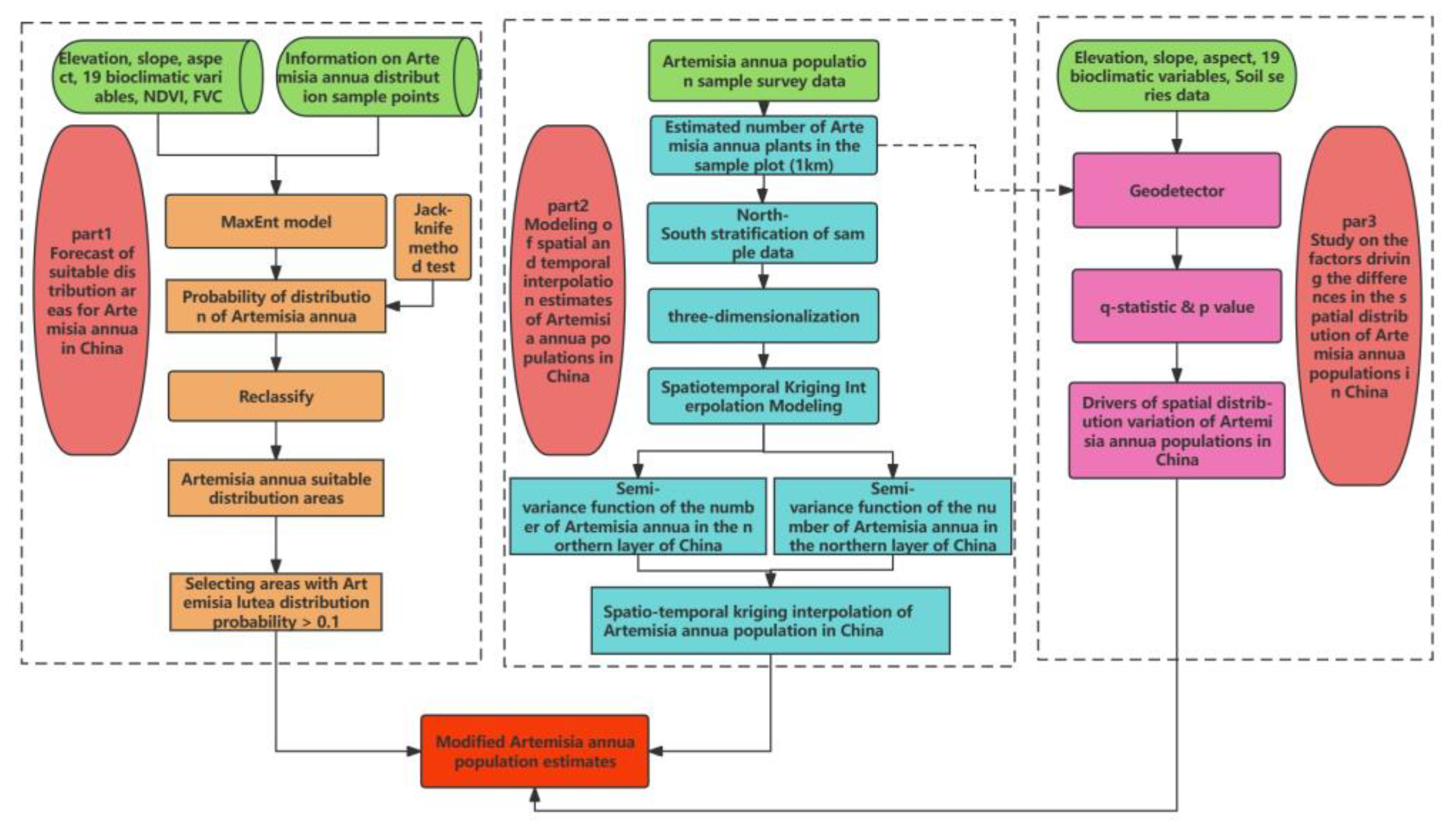
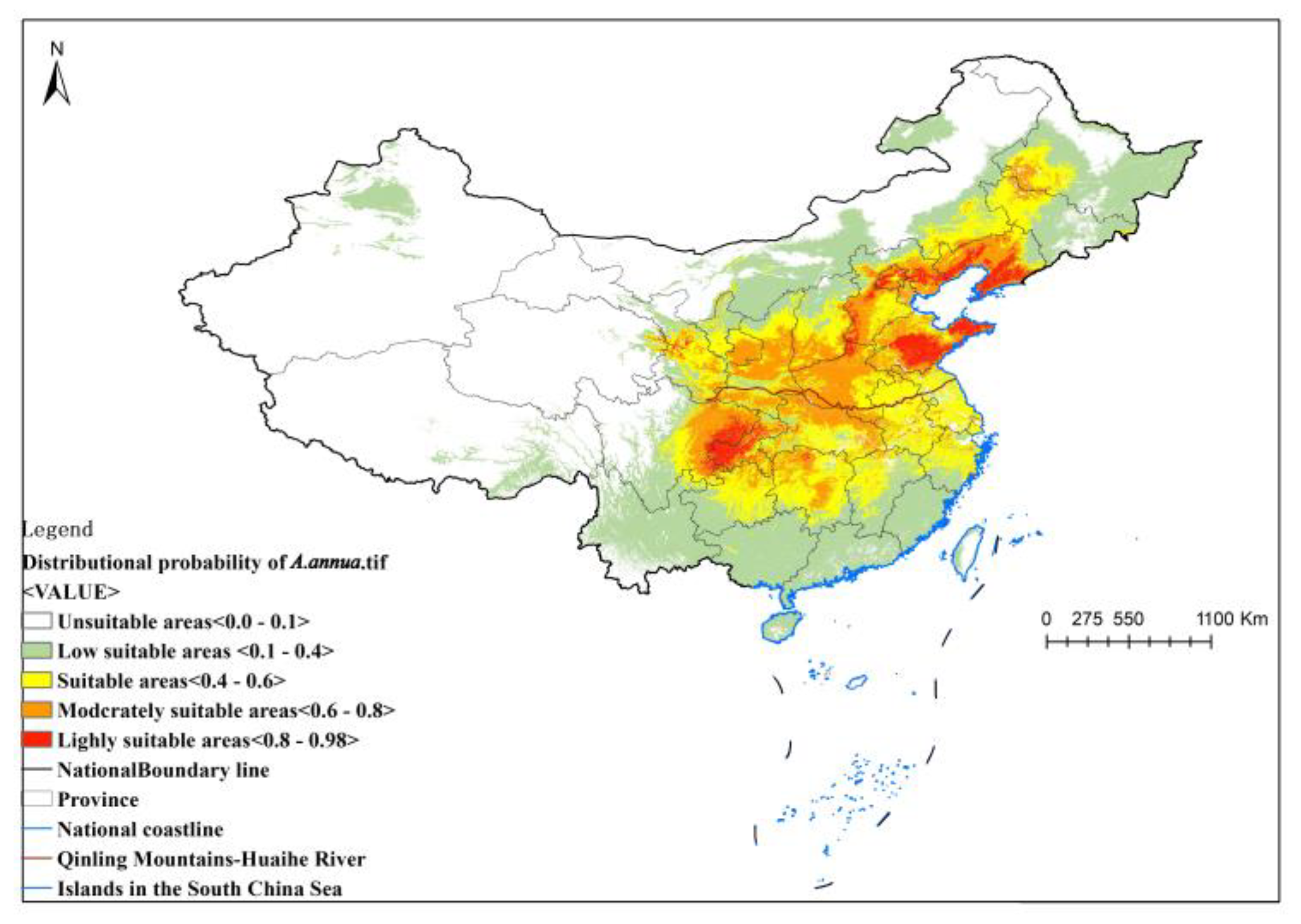
In the first step, we collected data on the distribution points and environmental variables of A. annua and studied the distribution of suitable areas based on Maxent modeling. The result was the suitable distribution probabilities in each area.
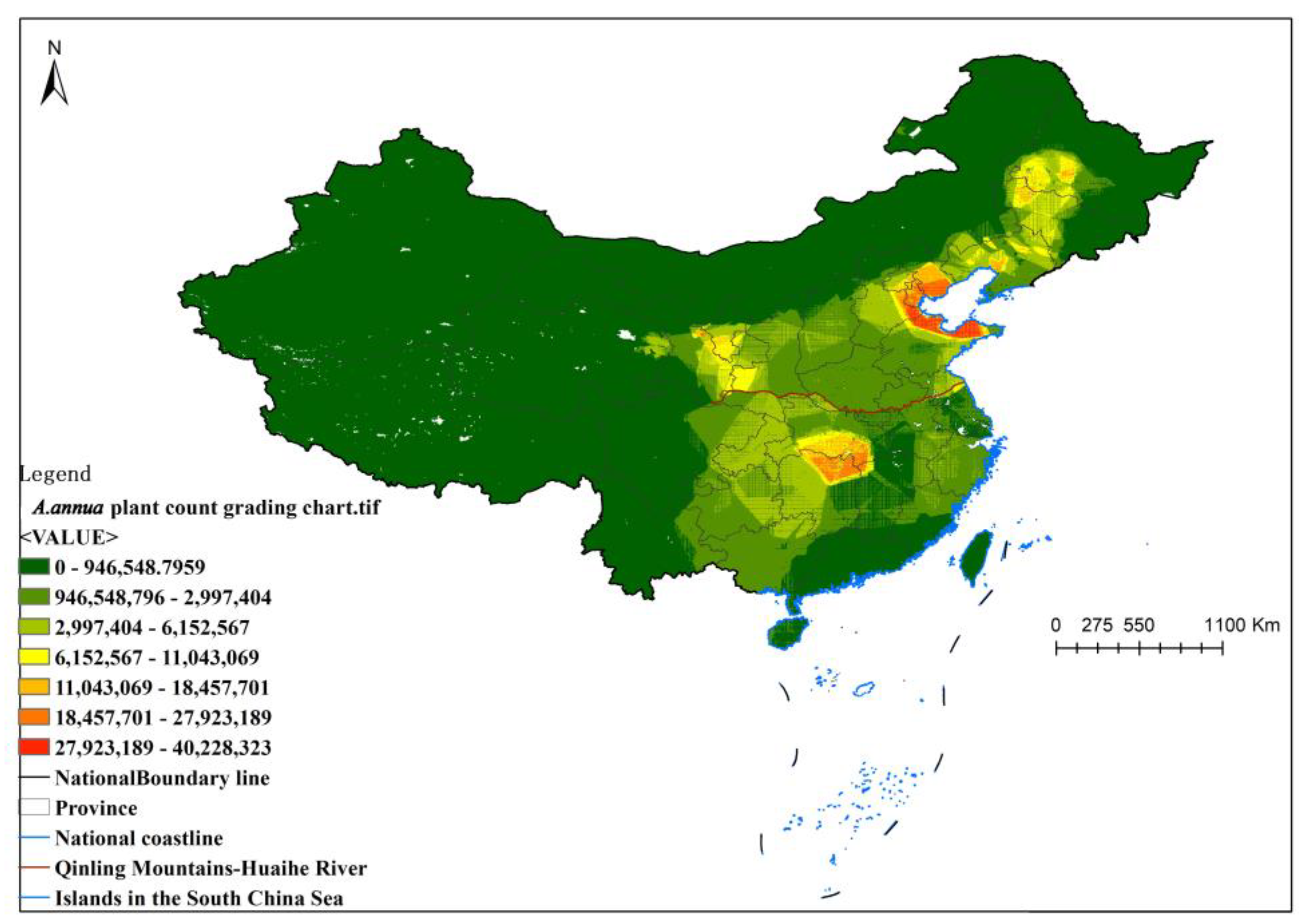
In the second step, based on the sample data of the number from the sample plot survey, we constructed a spatio-temporal kriging interpolation model of sample stratification and a semi-variate function study and estimated the amount. In the final Maxent result, a 100 km × 100 km national systematic sampling was carried out, and the points with a distribution probability less than 0.1 were screened out as correction points. The number of plants in these points was set to 0, and the remaining points were used for the estimation of the final number of plants.
In the third step, the factors affecting the differences in the spatial distribution were revealed using Geodetector.
4.2.1. Method for Studying the Ecologically Suitable Areas of A. annua in China
Ecologically suitable areas of
A. annua in China were determined using the MaxEnt (maximum entropy) method. The theory of maximum entropy was first proposed in 1957 [
31]. The Java MaxEnt model, which was developed from this theory, has become the most commonly used species distribution model (SDM). MaxEnt is a density estimation and species distribution prediction model based on the maximum entropy theory, which has the advantages of stable results and a short operation time. It is widely used in the analysis of plant and animal growth environments, pest early warning systems, habitat protection and the prediction of potential distribution areas [
32,
33]. It also has a wide range of applications in the prediction of potential ecologically suitable ranges of species, the effects of climate change on species distributions [
41], and the conservation of endangered species [
42].
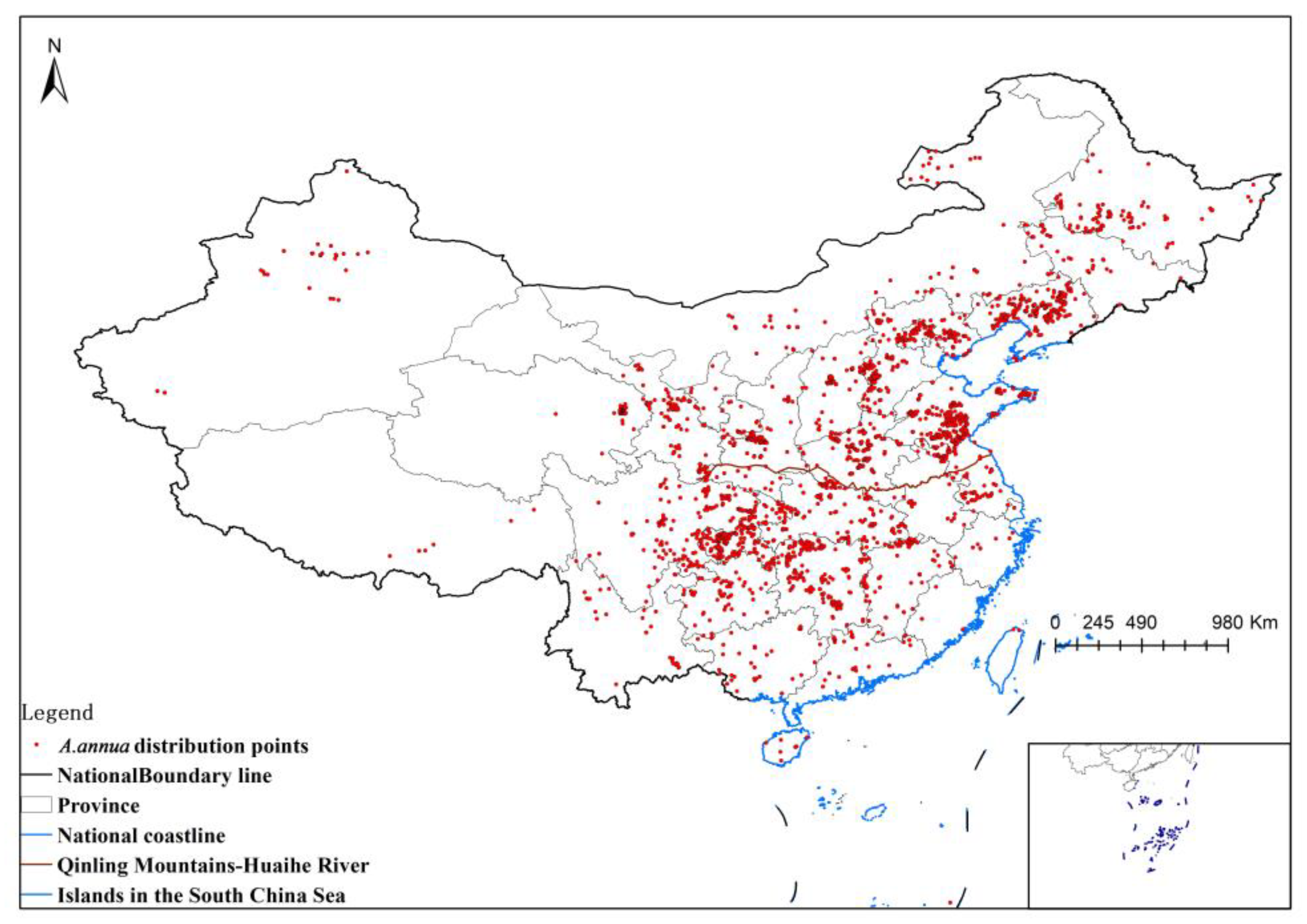
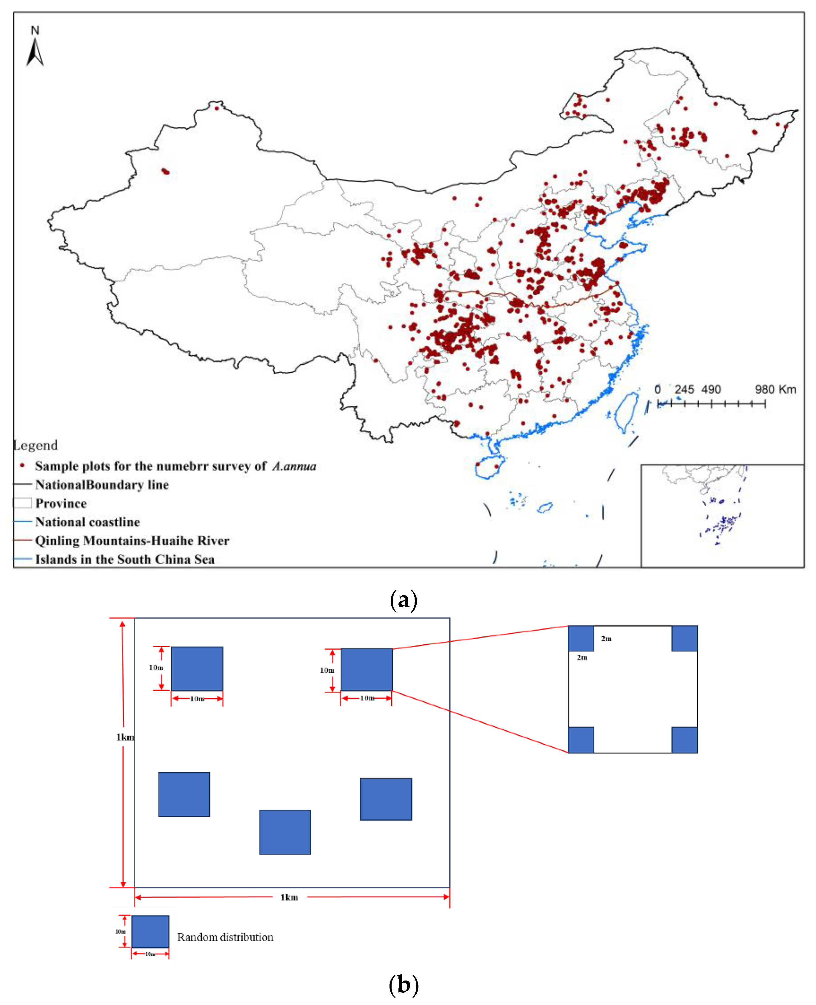
The distribution points and environmental variables were saved as .csv data in the order of species name, longitude, and latitude and imported into MaxEnt 3.4.4 software for modeling. We randomly selected 75% of the distribution points as the training set and 25% as the test set. The maximum number of iterations was set to 1000, and the subsample method was selected to repeat the runs to create different test and validation sets. The calculation was repeated 10 times, the jack-knife method was employed to calculate the influence of environmental variables on the distribution, and the response curve of each environmental variable was drawn. The results were output in logistic form in .asc format, where the raster value was the probability of survival (p-value). The output results were converted to raster format in ArcMap 10.8.
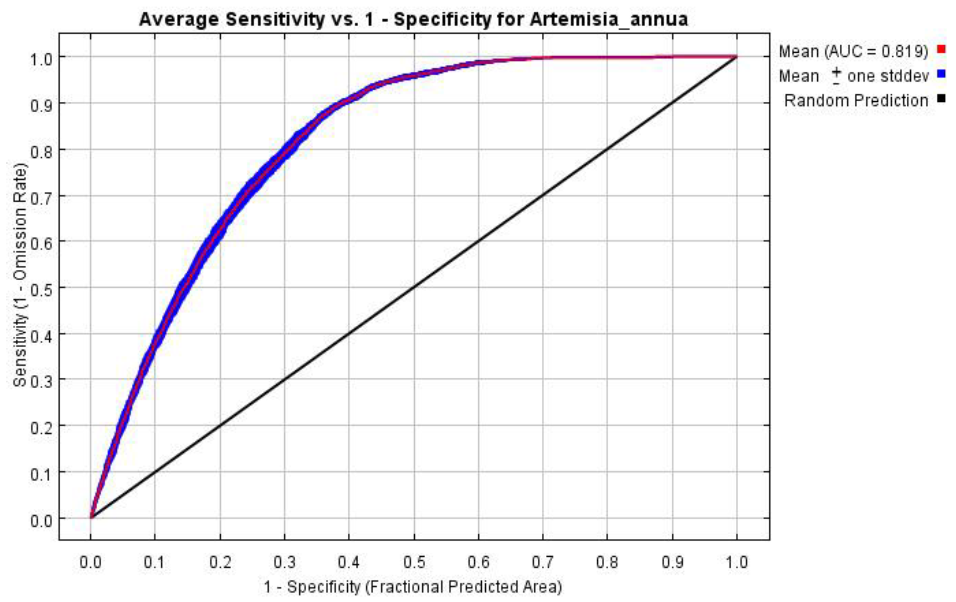
The prediction results of the MaxEnt model were evaluated by the range of the AUC (area under curve), which is the area under the receiver operating characteristic (ROC) curve plotted with the specificity as the horizontal coordinate and the sensitivity as the vertical coordinate. The range of the AUC is 0–1, where the larger value means the further away from the random distribution and the better the prediction result. The value of the AUC is generally between 0 and 1, where an AUC value between 0 and 0.5 indicates that the model prediction failed; an AUC value between 0.6 and 0.7 indicates that the prediction effect is poor; an AUC value between 0.7 and 0.8 indicates that the prediction effect is general; an AUC value between 0.8 and 0.9 indicates that the prediction effect is satisfying; and an AUC value greater than 0.9 indicates that the prediction effect is good [
43].
4.2.2. Method for Estimating the of Amount A. annua in China
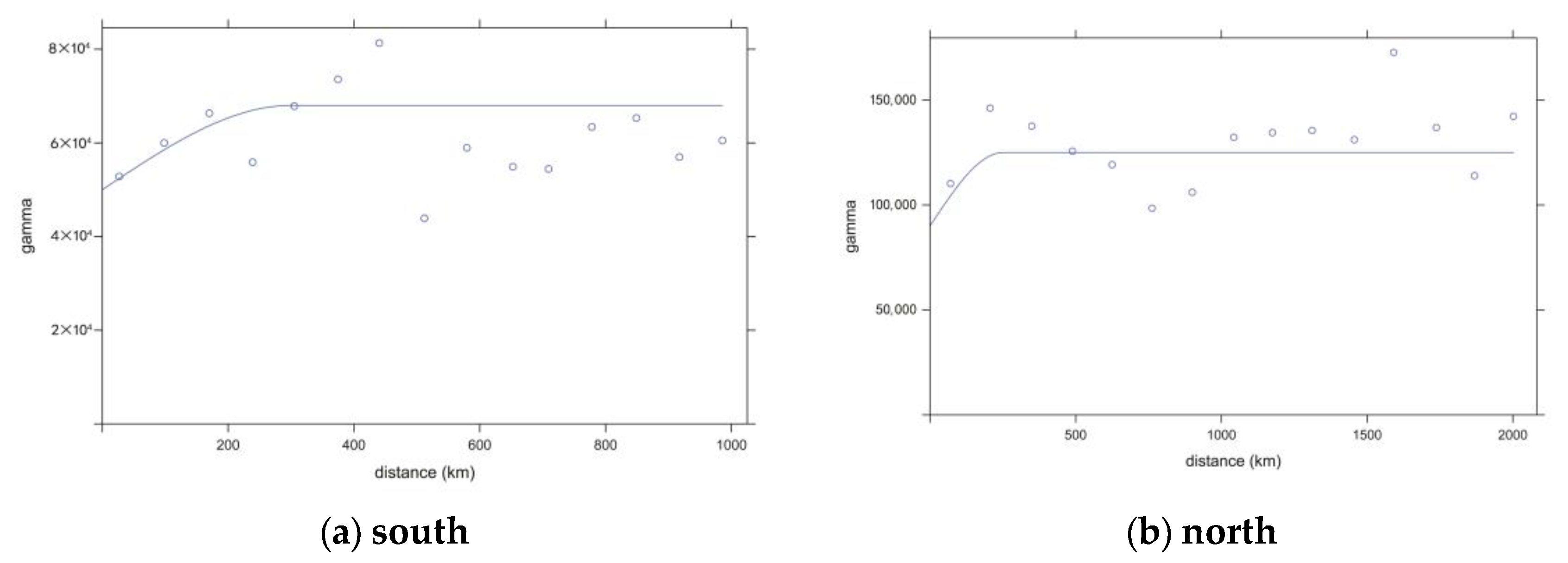
Data stratification: All collected sample data were stratified using the Geodetector method, which stratified the data according to the southern and northern regions of China, according to the month in which the data were collected and according to the season; analysis was conducted based on q-values and p-values.
The GeoDetector model uses the q-statistic to quantify the determinant powers of the influencing factors from spatio-temporal perspectives and the stratified heterogeneity of a dependent variable [
25,
44]. It is expressed as follows:
where
q is the determining power of the environmental factor, which takes values ranging from 0 to 1 and represents the determinant power of the heterogeneity of the risk factor or target variable.
(
= 1, 2, …, L) denotes the spatial stratification of a single factorization X.
and
are the numbers of units in the entire area and stratum
, respectively.
and
are the variances in the number of
A. annua specimens in the entire area and stratum h, respectively.
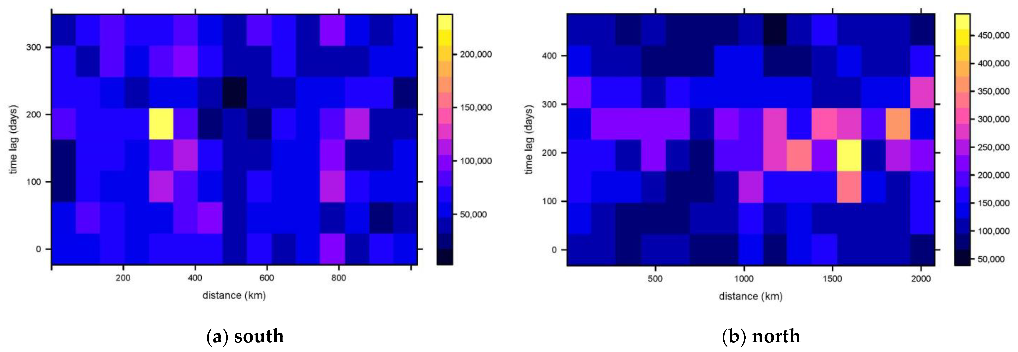
Three-dimensionalization: The year at the time of collection of all sample points is transformed into a spatial z-value, which forms a three-dimensional coordinate with latitude and longitude. The anisotropy coefficient of year and spatial distance (unit: km/month) is equal to the ratio of the variance in the spatio-temporal semi-variance function of the samples in each stratum. Since
A. annua is harvested during the flowering period as a raw material for artemisinin extraction, and it flowers from July to September [
34,
45], the month with the largest number of samples, July 2019, was chosen as the reference point and set as the time origin in this study.
The modeling process of the spatio-temporal kriging interpolation method is as follows:
Assumption 1: In order to increase the sample information, all the count data from 2012 to 2020 are assumed to be the background value samples in China.
Assumption 2: The number of A. annua per km2 in China is a random variable and satisfies the second-order smooth assumption. The expectation of the number of plants at any point in space is the same, and the covariance of the number of plants at any two points is related to their distances rather than to their spatial locations.
The basic principle is as follows:
The number of plants in space is represented as a random variable
, and the number of plants at any point can be represented as the sum of the weights of the surrounding sample points.
where
denotes the number of plants at the point to be measured,
denotes the number of sample points,
denotes the weighted contribution of sample point
to the point to be measured at time
and
denotes the number of
A. annua specimens in the measured sample.
A spatio-temporal semi-variogram is an index describing the spatial relationship characteristics of spatially random variables, and the empirical semi-variogram is calculated from two points in spatio-temporal distance H.
where
H is the spatio-temporal distance,
h is the Euclidean spatial distance between two points,
u is the time interval between two points,
k is the spatio-temporal anisotropy, and
N(
H) represents the number of sample point pairs at each spatio-temporal distance. Under the constraint of unbiased optimality, the system of equations can be obtained:
By solving the equation, the weighted contribution of each sample point to the measurement point can be obtained and then substituted into Equation (7) to calculate the number of trees to be measured.
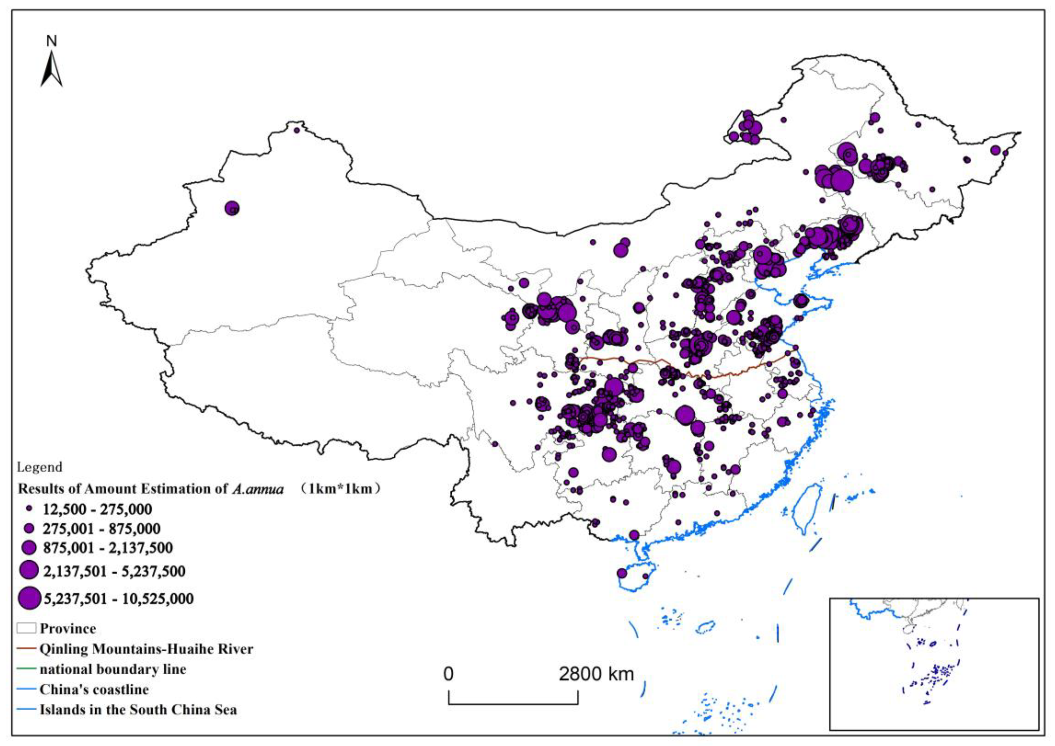
Since the spatial modeling assumes a certain constant expectation of strain counts across the country, it defies reality. Therefore, it is necessary to correct the strain count at each predicted site via ecological modeling. In this study, the MaxEnt model was used to estimate the probability of species distribution using covariates (19 climatic BIO variate factors, topographic factors of elevation, slope and slope direction data, monthly precipitation, monthly mean temperature, monthly minimum temperature, monthly maximum temperature, normalized vegetation index, and vegetation cover data) for the whole country in 1 km × 1 km plots.
In the final MaxEnt results, a 100 km × 100 km national systematic sampling was conducted to screen out the points with distribution probabilities less than 0.1 as correction points, and their amounts were set to 0 in the estimation of the final plant counts to ensure reasonable fit in the spatial prediction. At the same time, the points at which the distribution probability of the sample was less than 0.1 were removed and not involved in the calculation.
After fitting the model with sampled data, each data point is removed from the sampled dataset one at a time. Then, the leave-one-out dataset [
46] is applied to the model to estimate the value at the removed point. The estimate is compared with the observed true value by calculating the experimental error. In this paper, the mean absolute error (MAE) and root-mean-square error (RMSE) are evaluated [
47].
where
denotes the observed value of
A. annua at the
sample site,
represents the estimated value of the
sample site, and
n is the number of observations. A smaller
RMSE indicates a more precise interpolation model.
We also used the
MSE to evaluate the validity of our methods. The
MSE is usually used to describe the degree of change in the data and is expressed as
where
denotes the observed value of
A. annua at the
sample site,
represents the estimated value at sample site
, and
n is the number of observations.
Geodetector q-statistics were used to explore the main influencing factors affecting the amount. The influencing role is expressed as the influence strength, as a q value of [0, 1], where a value closer to 0 indicates that the factor has a weaker influence, and closer to 1, the influence is stronger. In this paper, 19 climate variables, topographic factors (elevation, slope, slope direction), soil factors (soil type, soil Ph, soil clay content, soil sand content, soil effective water content), and vegetation type factors were selected as potential influencing factors to analyze the distribution based on geodetic probes. The number estimated from 1579 sample plots was used as the most dependent variable Y, and the extracted environmental variable data were used as the independent variables X. The above independent variables were discretized by removing the variables of soil type and vegetation type and then run in GeoDetector software (2015_Example) to assess the factors influencing the differences in the spatial distribution.


