
Monitoring Plant Height and Spatial Distribution of Biometrics with a Low-Cost Proximal Platform


 , , ,
, , ,  ,
,  , ,
, ,  and
and
Abstract
1. Introduction
2. Results
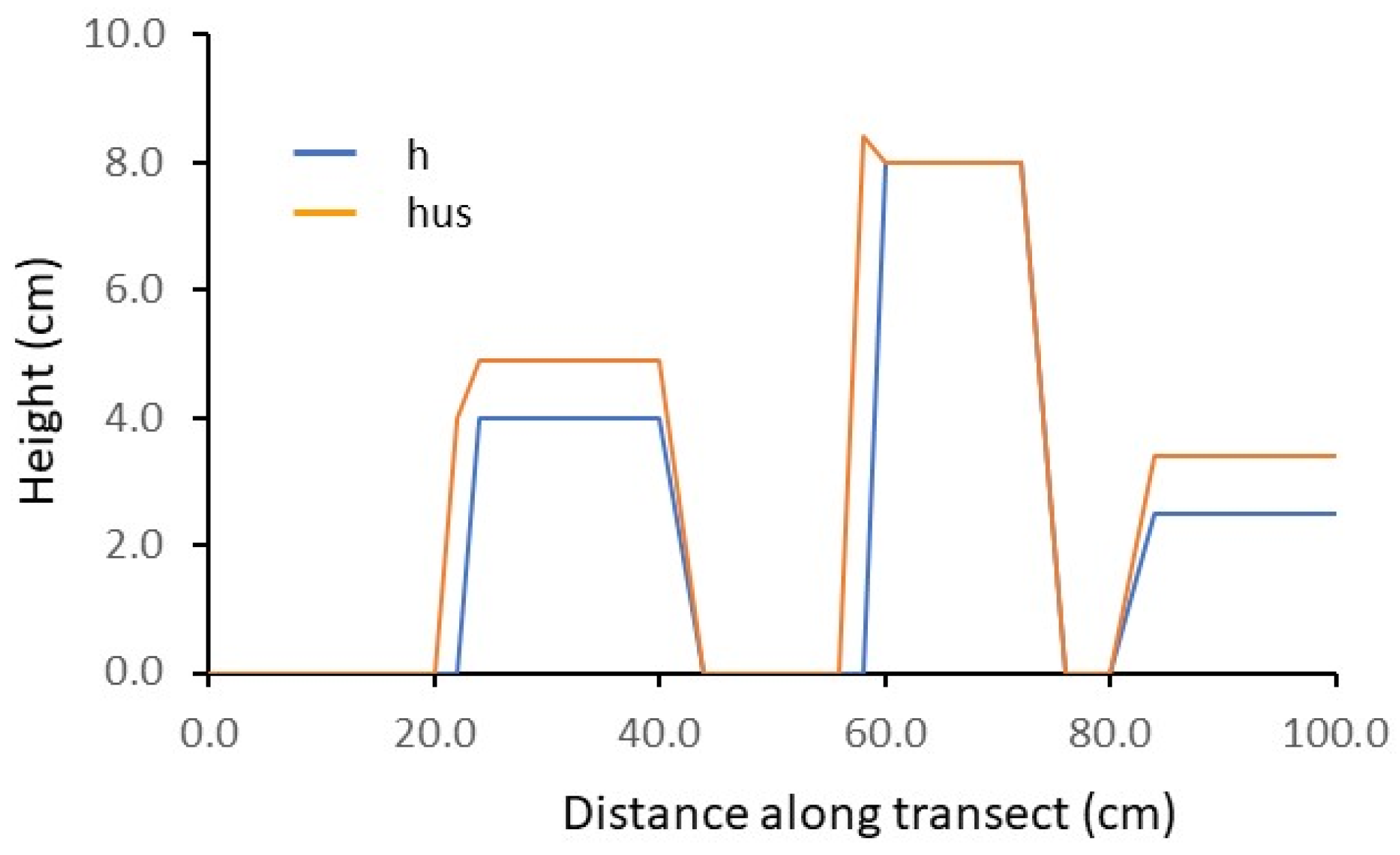
2.1. Lab Tests
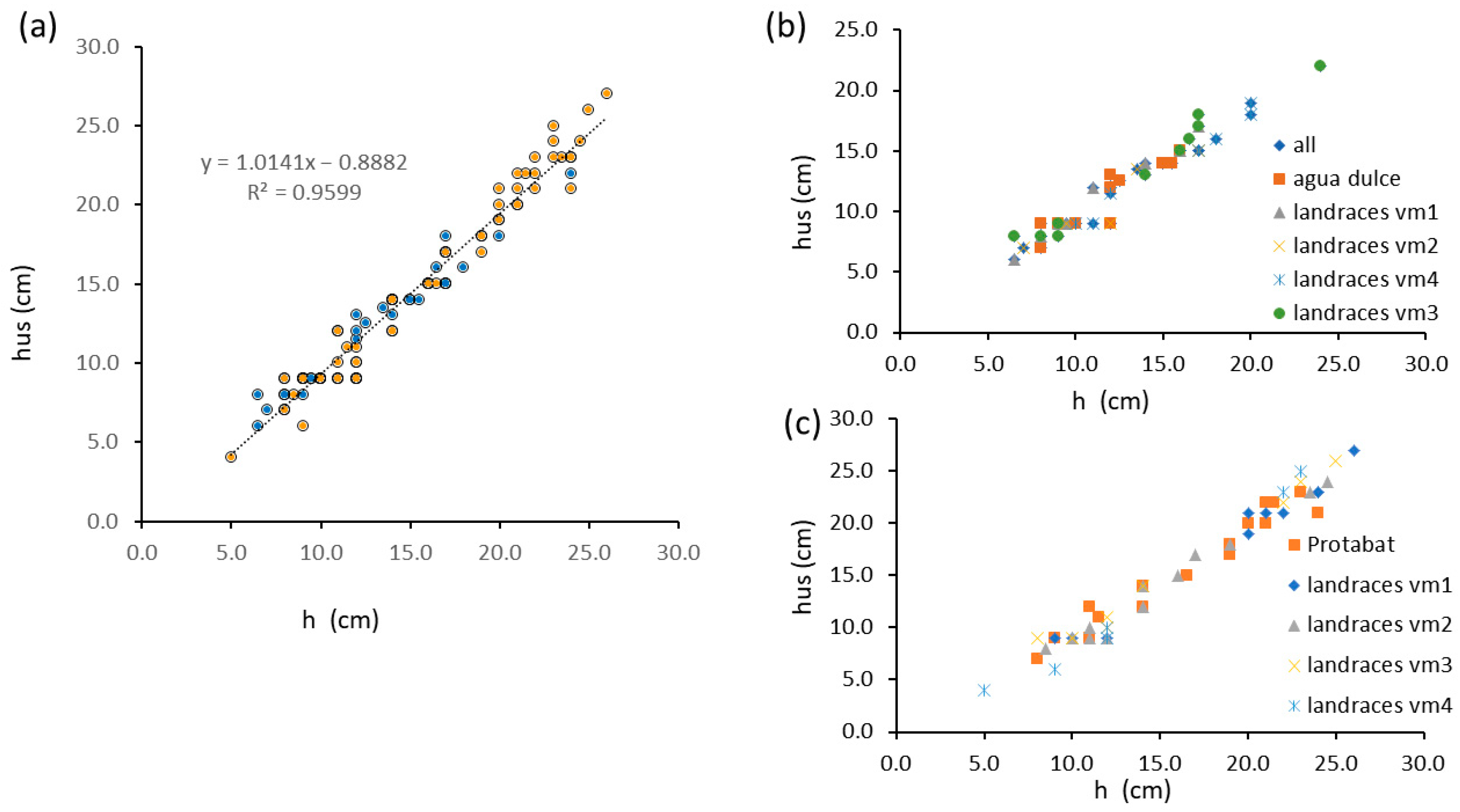
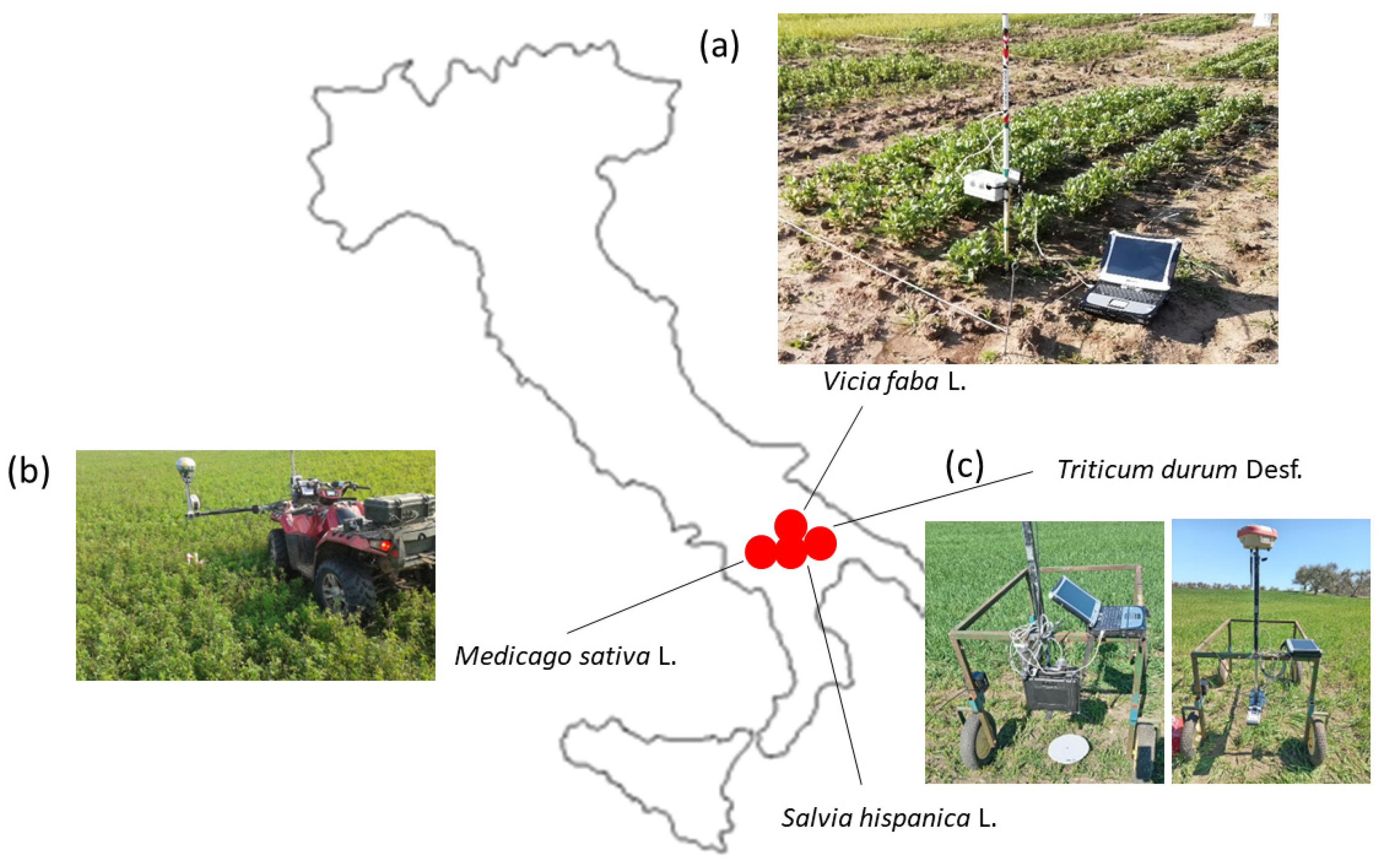
2.2. Faba Bean (Vicia faba L.)
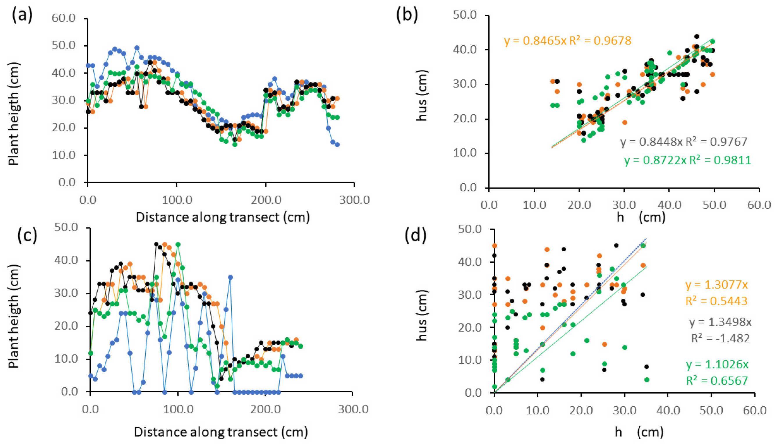
2.3. Chia (Salvia hispanica L.)
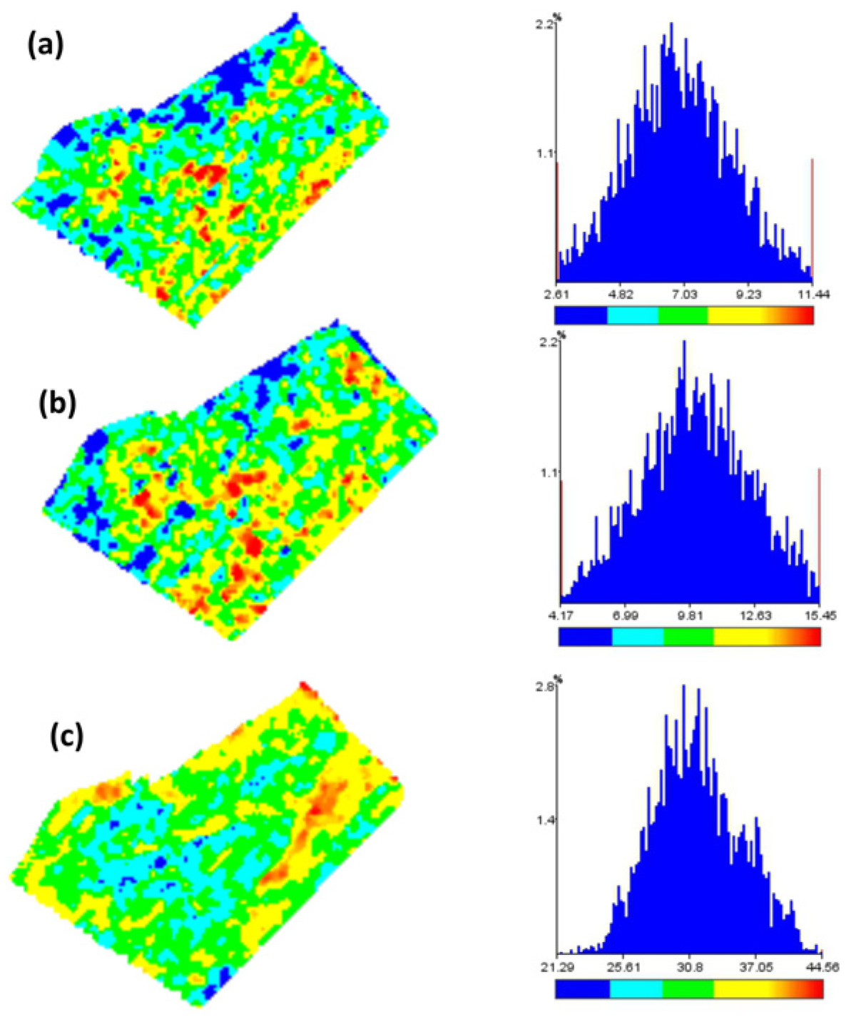
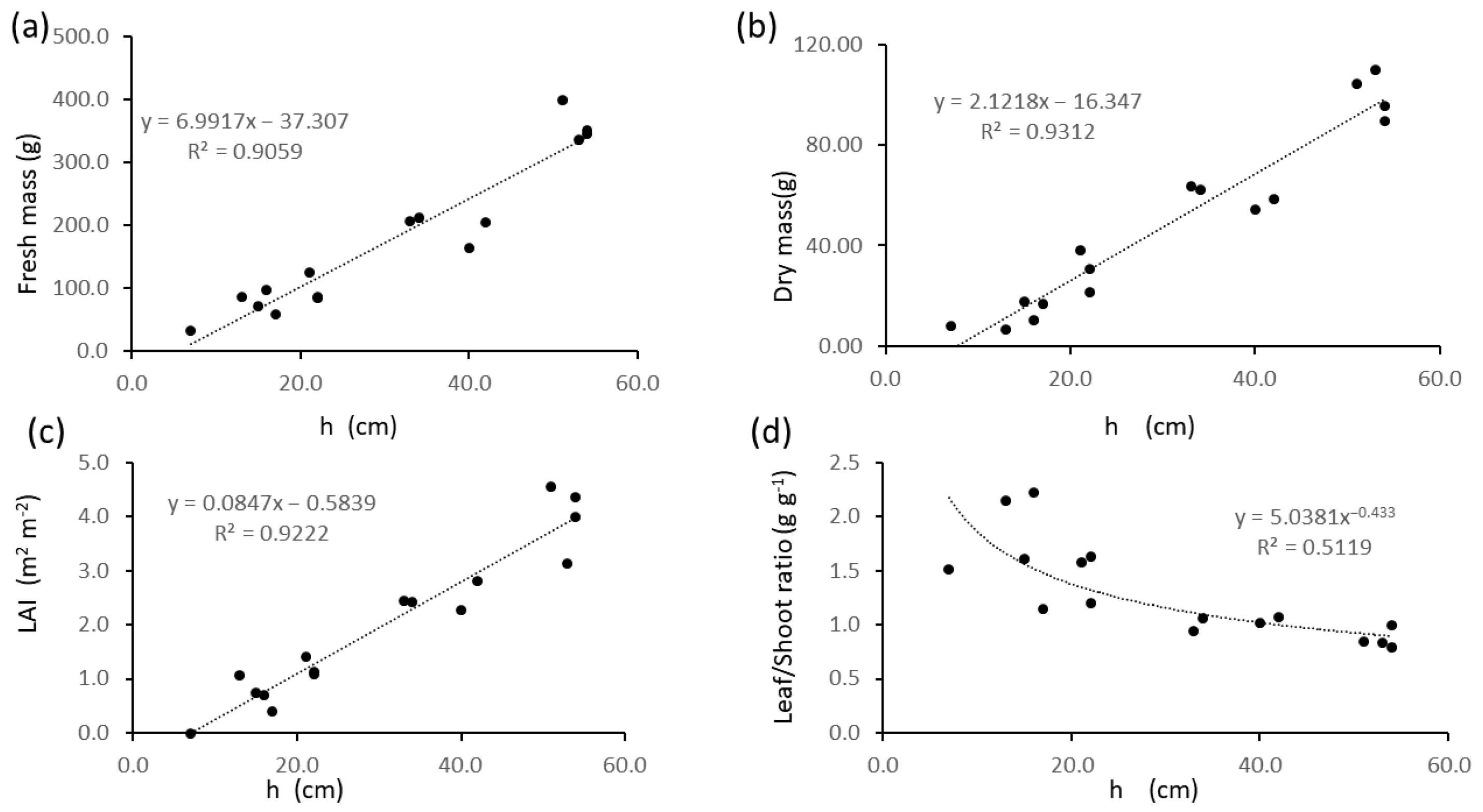
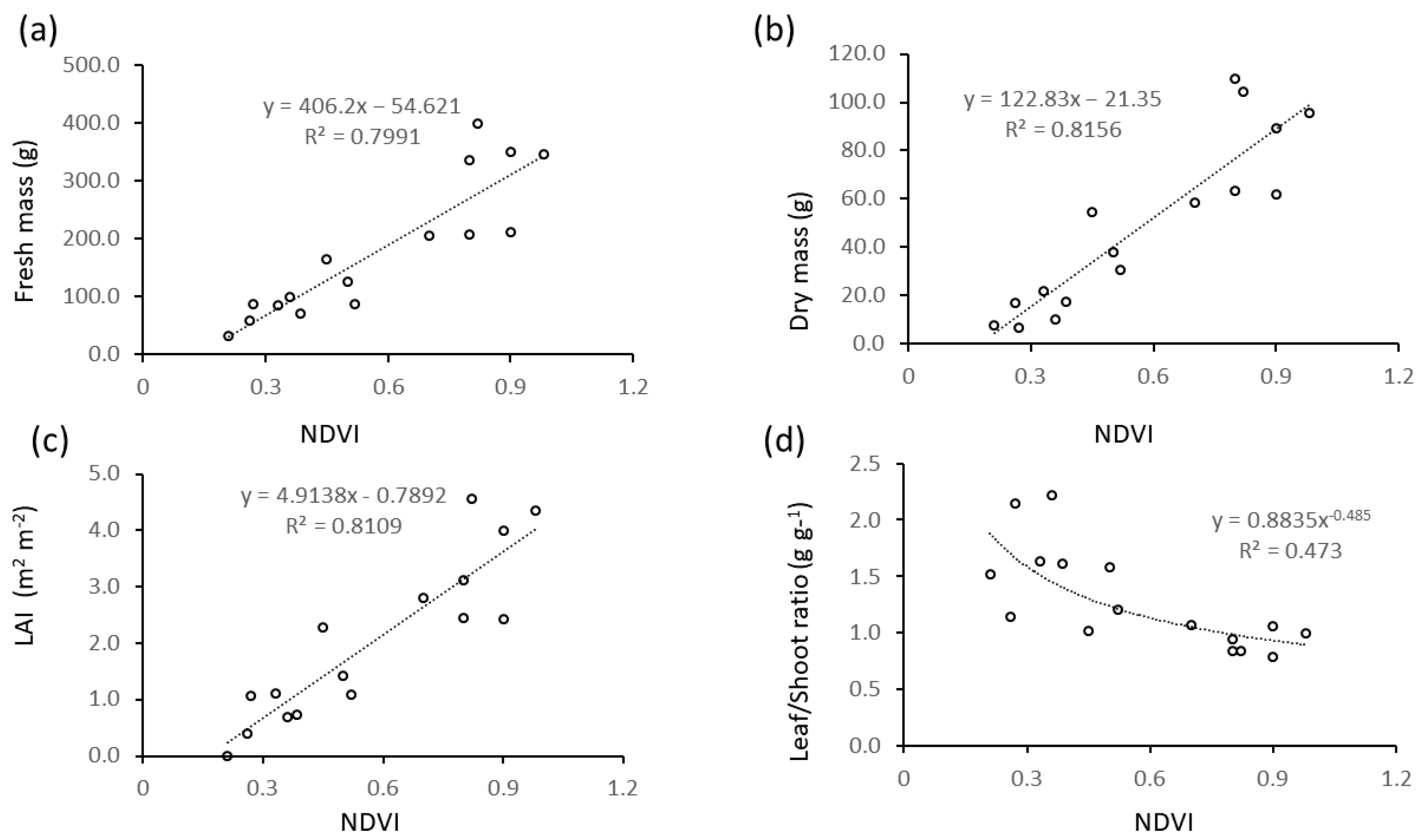
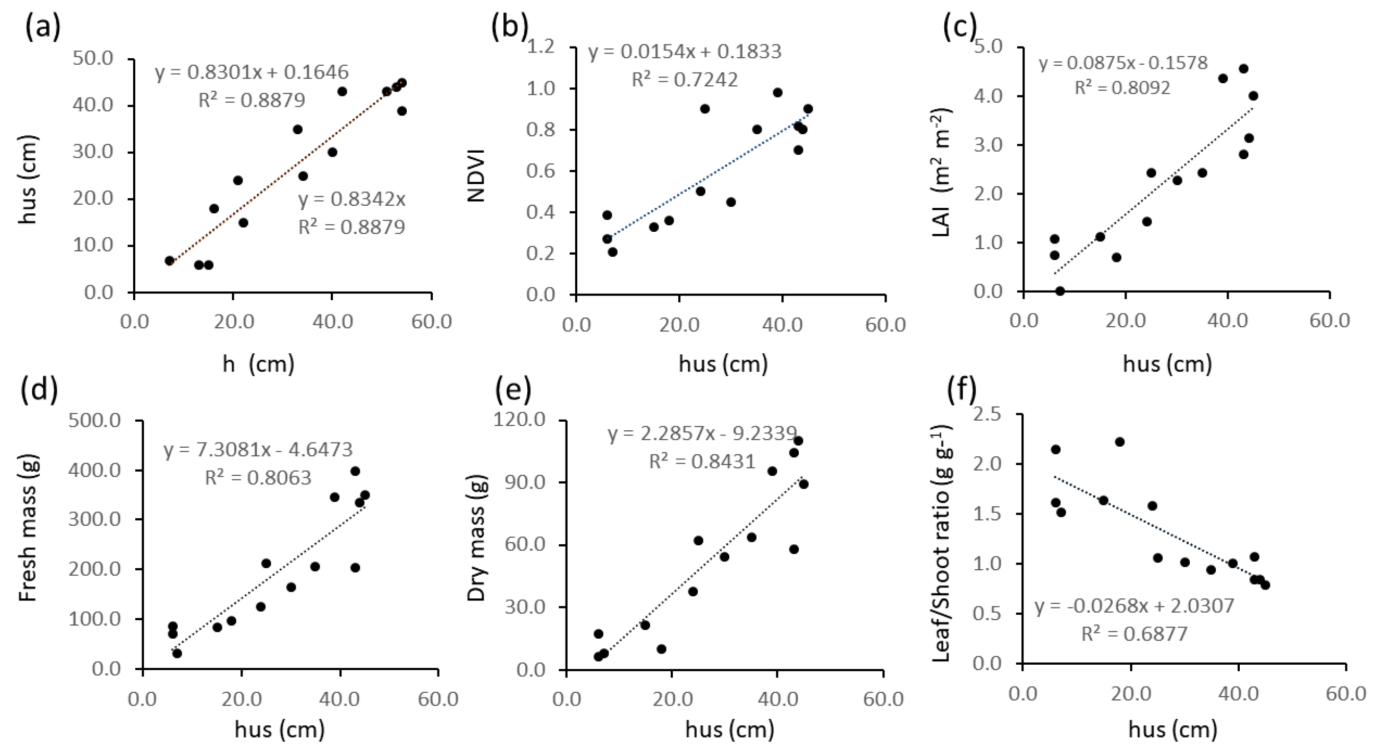
2.4. Alfalfa (Medicago sativa L.)
2.5. Wheat (Triticum durum Desf.)
3. Discussion
4. Materials and Methods
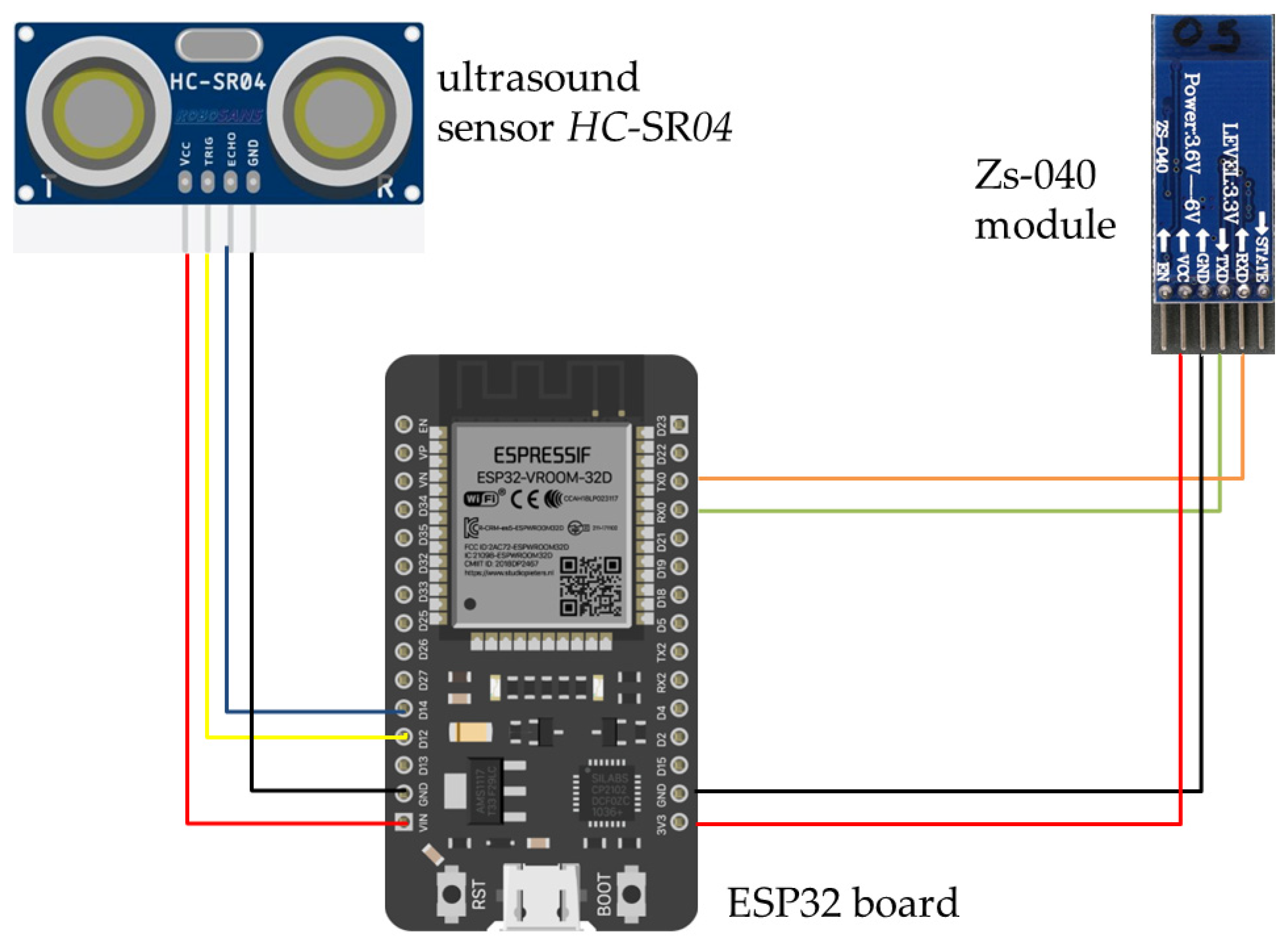
4.1. Ultrasound Sensor Platform
- (1)
- An ESP32 board (Espressif Systems, Singapore) with a dual-core microcontroller. Tensilica Xtensa 32-bit LX6 microprocessor with wireless connectivity Wi-Fi: 802.11 b/g/n/e/i (802.11n @ 2.4 GHz up to 150 Mbit/s) and Bluetooth: v4.2 BR/EDR and Bluetooth Low Energy (BLE). The current cost of an ESP32 board ranges from 1.75 to 8 Euros depending on the source.
- (2)
- An ultrasound sensor was an HC-SR04 (Picaxe, Revolution Education Ltd, Bathh, UK) transmitting at 40 KHz frequency, and operating between 3 and 400 cm of distance with accuracy of 3 mm with a cone of 45 degrees from the sensor. The HC-SR04 rapidly generates a series of ultrasound pulses which propagate in a straight line in front of the sensor. The ultrasounds hit an object in front of the sensor and are reflected back towards the sensor, which detects the time taken for the ultrasound pulses to travel from their source to the object and back. The sensor uses the elapsed time to calculate the distance between itself and the object as:
- (3)
- A Zs-040 module which sends data via Bluetooth. This was added in order to simplify hardware and make data easily available in real time thanks to transmission to a PC or smartphone. The current cost ranges from 0.3 to 10 m Euros depending on the source.
4.2. Data Collection
4.3. Sensor Testing
4.3.1. Lab Test
4.3.2. Faba Bean (Vicia faba L.)
- Vma1 = Accession number 112906 from USA Vma1
- Vma2 = Accession number 103235 from Italy
- Vma3 = Accession number 107620 from Greece.
- Vma4 = Accession number 106374 from Algeria
- Vmi1 = Accession number 113620 from Germany
- Vmi2 = Accession number 113620 from Germany
- Vmi3 = Accession number 109322 from Ethiopia
- Vmi4 = Accession number 118952 from Afghanistan
4.3.3. Chia (Salvia hispanica L.)
4.3.4. Alfalfa (Medicago sativa L.)
NDVI
Leaf Area Index
Vegetation Height
Biomass
4.3.5. Wheat (Triticum durum Desf.)
4.4. Statistical Analysis
5. Conclusions
Author Contributions
Funding
Data Availability Statement
Conflicts of Interest
References
- Moles, A.T.; Warton, D.I.; Warman, L.; Swenson, N.; Laffan, S.W.; Zanne, A.; Pitman, A.J.; Hemmings, F.; Leishman, M. Global patterns in plant height. J. Ecol. 2009, 97, 923–932. [Google Scholar] [CrossRef]
- Heady, H.F. The Measurement and Value of Plant Height in the Study of Herbaceous Vegetation. Ecology 1957, 38, 313–320. [Google Scholar] [CrossRef]
- Westoby, M.; Falster, D.S.; Moles, A.T.; Vesk, P.A.; Wright, I.J. Plant ecological strategies: Some leading dimensions of variation between species. Ann. Rev. Ecol. Syst. 2002, 33, 125–159. [Google Scholar] [CrossRef]
- Proulx, R. On the general relationship between plant height and aboveground biomass of vegetation stands in contrasted ecosystems. PLoS ONE 2021, 16, e0252080. [Google Scholar] [CrossRef] [PubMed]
- Yin, X.; McClure, M.A.; Jaja, N.; Tyler, D.D.; Hayes, R.M. In-season prediction of corn yield using plant height under major production systems. Agron. J. 2011, 103, 923–929. [Google Scholar] [CrossRef]
- Mourtzinis, S.; Arriaga, F.J.; Balkcom, K.S.; Ortiz, B.V. Corn grain and stover yield prediction at R1 growth stage. Agron. J. 2013, 105, 1045–1050. [Google Scholar] [CrossRef]
- Cui, F.; Li, J.; Ding, A.; Zhao, C.; Wang, L.; Wang, X.; Li, S.; Bao, Y.; Li, X.; Feng, D.; et al. Conditional QTL mapping for plant height with respect to the length of the spike and internode in two mapping populations of wheat. Theor. Appl. Genet. 2011, 122, 1517–1536. [Google Scholar] [CrossRef] [PubMed]
- Boomsma, C.R.; Santini, J.B.; West, T.D.; Brewer, J.C.; McIntyre, L.M.; Vyn, T.J. Maize grain yield responses to plant height variability resulting from crop rotation and tillage system in a long-term experiment. Soil Till. Res. 2010, 106, 227–240. [Google Scholar] [CrossRef]
- Machado, S.; Bynum, E.D.; Archer, T.L.; Lascano, R.J.; Wilson, L.T.; Bordovsky, J.; Segarra, E.; Bronson, K.; Nesmith, D.M.; Xu, W. Spatial and temporal variability of corn growth and grain yield. Crop Sci. 2002, 42, 1564–1576. [Google Scholar] [CrossRef]
- Dandois, J.P.; Ellis, E.C. High spatial resolution three-dimensional mapping of vegetation spectral dynamics using computer vision. Remote Sens. Environ. 2013, 136, 259–276. [Google Scholar] [CrossRef]
- Jin, J.; Tang, L. Corn plant sensing using real-time stereo vision. J. Field Robot. 2009, 26, 591–608. [Google Scholar] [CrossRef]
- Baha, N. Real-Time Obstacle Detection Approach using Stereoscopic Images. Int. J. Inf. Eng. Electron. Bus. 2014, 6, 42–48. [Google Scholar] [CrossRef][Green Version]
- Omasa, K.; Hosoi, F.; Konishi, A. 3D lidar imaging for detecting and understanding plant responses and canopy structure. J. Exp. Bot. 2014, 58, 881–898. [Google Scholar] [CrossRef] [PubMed]
- Saeys, W.; Lenaerts, B.; Craessaerts, G.; De Baerdemaeker, J. Estimation of the crop density of small grains using LiDAR sensors. Biosyst. Eng. 2009, 102, 22–30. [Google Scholar] [CrossRef]
- Andújar, D.; Escolà, A.; Rosell-Polo, J.R.; Fernández-Quintanilla, C.; Dorado, J. Potential of a terrestrial LiDAR-based system to characterise weed vegetation in maize crops. Comput. Electron. Agric. 2013, 92, 11–15. [Google Scholar] [CrossRef]
- Fricke, T.; Richter, F.; Wachendorf, M. Assessment of forage mass from grassland swards by height measurement using an ultrasonic sensor. Comput. Electron. Agric. 2011, 79, 142–152. [Google Scholar] [CrossRef]
- Llorens, J.; Gil, E.; Llop, J.; Queraltó, M. Georeferenced LiDAR 3D vine plantation map generation. Sensors 2011, 11, 6237–6256. [Google Scholar] [CrossRef] [PubMed]
- Andújar, D.; Weis, M.; Gerhards, R. An ultrasonic system for weed detection in cereal crops. Sensors 2012, 12, 17343–17357. [Google Scholar] [CrossRef] [PubMed]
- Fisher, D.K.; Gould, P.J. Open-Source Hardware Is a Low-Cost Alternative for Scientific Instrumentation and Research. Mod. Instrum. 2012, 1, 8–20. [Google Scholar] [CrossRef]
- Leeuw, T.; Boss, E.S.; Wright, D.L. In situ measurements of phytoplankton fluorescence using low cost electronics. Sensors 2013, 13, 7872–7883. [Google Scholar] [CrossRef]
- Bronson, K.F.; French, A.N.; Conley, M.M.; Barnes, E.M. Use of an Ultrasonic Sensor for Plant Height Estimation in Irrigated Cotton. Agron. J. 2021, 113, 2175–2183. [Google Scholar] [CrossRef]
- Scotford, I.M.; Miller, P.C.H. Combination of Spectral Reflectance and Ultrasonic Sensing to Monitor the Growth of Winter Wheat. Biosyst. Eng. 2004, 87, 27–38. [Google Scholar] [CrossRef]
- Fisher, D.K.; Huang, Y. Mobile Open-Source Plant-Canopy Monitoring System. Mod. Instrum. 2017, 6, 1–13. [Google Scholar] [CrossRef][Green Version]
- Sui, R.; Thomasson, J.A.; Ge, Y. Development of Sensor Systems for Precision Agriculture in Cotton. Biol. Eng. 2012, 5, 14. [Google Scholar]
- Sharma, B.; Ritchie, G.L. High-Throughput Phenotyping of Cotton in Multiple Irrigation Environments. Crop Sci. 2015, 55, 958–969. [Google Scholar] [CrossRef]
- Barker, J.; Zhang, N.; Sharon, J.; Steeves, R.; Wang, X.; Wei, Y.; Poland, J. Development of a Field-Based High-Throughput Mobile Phenotyping Platform. Comput. Electron. Agric. 2016, 122, 74–85. [Google Scholar] [CrossRef]
- Andrade-Sanchez, P.; Gore, M.A.; Heun, J.T.; Thorp, K.R.; Carmo-Silva, A.E.; French, A.N.; Salvucci, M.E.; White, J.W. Development and Evaluation of a Field-Based High-Throughput Phenotyping Platform. Funct. Plant Biol. 2013, 41, 68–79. [Google Scholar] [CrossRef]
- Montazeaud, G.; Langrume, C.; Moinard, S.; Goby, C.; Ducanchez, A.; Tisseyre, B.; Brunel, G. Development of a low cost open-source ultrasonic device for plant height measurements. Smart Agric. Technol. 2021, 1, 100022. [Google Scholar] [CrossRef]
- Mori, U.; Mendiburu, A.; Lozano, J.A. Distance Measures for Time Series in R: The TSdist Package. R J. 2016, 8, 451. [Google Scholar] [CrossRef]
- Liao, W.T. Clustering of time series data—A survey. Pattern Recogn. 2005, 38, 1857–1874. [Google Scholar] [CrossRef]
- Sui, R.; Thomasson, J.A. Ground-based sensing system for cotton nitrogen status determination. Trans. ASABE 2006, 49, 1983–1991. [Google Scholar] [CrossRef]
- Aziz, S.A.; Steward, B.L.; Birrell, S.J.; Shrestha, D.S.; Kaspar, T.C. Ultrasonic sensing for corn plant canopy characterization. In Proceedings of the ASAE Annual Meeting, Ottawa, ON, USA, 15–18 August 2004; p. 041120. [Google Scholar]
- Jones, C.L.; Maness, N.O.; Stone, M.L.; Jayasekara, R. Sonar and digital imagery for estimating crop biomass. In Proceedings of the ASAE Annual Meeting, Ottawa, ON, USA, 15–18 August 2004; p. 04306. [Google Scholar]
- Fiorentino, C.; Donvito, A.R.; D’Antonio, P.; Lopinto, S. Experimental Methodology for Prescription Maps of Variable Rate Nitrogenous Fertilizers on Cereal Crops. In Innovative Biosystems Engineering for Sustainable Agriculture, Forestry and Food Production; Coppola, A., Di Renzo, G., Altieri, G., D’Antonio, P., Eds.; Lecture Notes in Civil Engineering; Springer: Cham, Switzerland, 2020; Volume 67. [Google Scholar] [CrossRef]
- Jeon, H.Y.; Zhu, H.; Derksen, R.; Ozkan, E.; Krause, C. Evaluation of ultrasonic sensor for variable-rate spray applications. Comput. Electron. Agric. 2011, 75, 213–221. [Google Scholar] [CrossRef]
- Legg, M.; Bradley, S. Ultrasonic Proximal Sensing of Pasture Biomass. Remote Sens. 2019, 11, 2459. [Google Scholar] [CrossRef]
- Lawson, H.F.; Giri, K.; Thomson, A.L.; Karunaratne, S.B.; Smith, K.F.; Jacobs, J.L.; Morse-McNabb, E.M. Multi-site calibration and validation of a wide-angle ultrasonic sensor and precise GPS to estimate pasture mass at the paddock scale. Comput. Electron. Agric. 2022, 195, 106786. [Google Scholar] [CrossRef]
- Duchemin, B.; Hadria, R.; Erraki, S.; Boulet, G.; Maisongrande, P.; Chehbouni, A.; Escadafal, R.; Ezzahar, J.; Hoedjes, J.C.B.; Kharrou, M.H.; et al. Monitoring wheat phenology and irrigation in Central Morocco: On the use of relationships between evapotranspiration, crops coefficients, leaf area index and remotely-sensed vegetation indices. Agric. Water Manag. 2006, 79, 1–27. [Google Scholar] [CrossRef]
- Zaman, Q.U.; Schumann, A.W.; Hostler, H.K. Quantifying sources of error in ultrasonic measurements of citrus orchards. Appl. Eng. Agric. 2007, 23, 449–453. [Google Scholar] [CrossRef]
- Bitella, G.; Rossi, R.; Bochicchio, R.; Perniola, M.; Amato, M. A Novel Low-Cost Open-Hardware Platform for Monitoring Soil Water Content and Multiple Soil-Air-Vegetation Parameters. Sensors 2014, 14, 19639–19659. [Google Scholar] [CrossRef] [PubMed]
- Lesch, S.M. Sensor-directed response surface sampling designs for characterizing spatial variation in soil properties. Comput. Electron. Agric. 2005, 46, 153–179. [Google Scholar] [CrossRef]
- Zadoks, J.C.; Chang, T.T.; Konzak, C.F. Decimal Code for the Growth Stages of Cereals. Weed Res. 1974, 14, 415–421. [Google Scholar] [CrossRef]
- R Core Team. R: A Language and Environment for Statistical Computing; R Foundation for Statistical Computing: Vienna, Austria, 2021; Available online: https://www.R-project.org/ (accessed on 3 September 2023).


| LAI of Alfalfa | Fresh Biomass | Dry Biomass | NDVI | Leaf/Total Mass Ratio | h | hus | |
|---|---|---|---|---|---|---|---|
| (m2 m−2) | (g m−2) | (g m−2) | (g g−1) | (cm) | (cm) | ||
| Min | 0 | 128.00 | 26.40 | 0.21 | 0.44 | 13.02 | 6.11 |
| Max | 4.56 | 1592.00 | 440.00 | 0.98 | 0.69 | 54.28 | 45.07 |
| Mean | 2.03 | 714.25 | 196.65 | 0.57 | 0.55 | 32.47 | 27.14 |
| St dev | 1.44 | 479.58 | 143.55 | 0.26 | 0.08 | 15.56 | 14.84 |
| CV% | 47.91 | 67.14 | 73.00 | 45.92 | 14.44 | 47.91 | 54.66 |
| hus | h | NDVI | LAI | |
|---|---|---|---|---|
| (cm) | (cm) | (m2 m−2) | ||
| Min | 5.53 | 6.02 | 0.10 | 0.32 |
| Max | 24.57 | 24.92 | 0.26 | 2.02 |
| Mean | 13.68 | 14.37 | 0.18 | 1.02 |
| St dev | 7.02 | 7.24 | 0.08 | 0.61 |
| CV% | 51.27 | 50.41 | 42.89 | 60.19 |
Disclaimer/Publisher’s Note: The statements, opinions and data contained in all publications are solely those of the individual author(s) and contributor(s) and not of MDPI and/or the editor(s). MDPI and/or the editor(s) disclaim responsibility for any injury to people or property resulting from any ideas, methods, instructions or products referred to in the content. |
© 2024 by the authors. Licensee MDPI, Basel, Switzerland. This article is an open access article distributed under the terms and conditions of the Creative Commons Attribution (CC BY) license (https://creativecommons.org/licenses/by/4.0/).
Share and Cite
Bitella, G.; Bochicchio, R.; Castronuovo, D.; Lovelli, S.; Mercurio, G.; Rivelli, A.R.; Rosati, L.; D’Antonio, P.; Casiero, P.; Laghetti, G.; et al. Monitoring Plant Height and Spatial Distribution of Biometrics with a Low-Cost Proximal Platform. Plants 2024, 13, 1085. https://doi.org/10.3390/plants13081085
Bitella G, Bochicchio R, Castronuovo D, Lovelli S, Mercurio G, Rivelli AR, Rosati L, D’Antonio P, Casiero P, Laghetti G, et al. Monitoring Plant Height and Spatial Distribution of Biometrics with a Low-Cost Proximal Platform. Plants. 2024; 13(8):1085. https://doi.org/10.3390/plants13081085
Chicago/Turabian StyleBitella, Giovanni, Rocco Bochicchio, Donato Castronuovo, Stella Lovelli, Giuseppe Mercurio, Anna Rita Rivelli, Leonardo Rosati, Paola D’Antonio, Pierluigi Casiero, Gaetano Laghetti, and et al. 2024. "Monitoring Plant Height and Spatial Distribution of Biometrics with a Low-Cost Proximal Platform" Plants 13, no. 8: 1085. https://doi.org/10.3390/plants13081085
APA StyleBitella, G., Bochicchio, R., Castronuovo, D., Lovelli, S., Mercurio, G., Rivelli, A. R., Rosati, L., D’Antonio, P., Casiero, P., Laghetti, G., Amato, M., & Rossi, R. (2024). Monitoring Plant Height and Spatial Distribution of Biometrics with a Low-Cost Proximal Platform. Plants, 13(8), 1085. https://doi.org/10.3390/plants13081085