4.1. Open-Field Experiment
Our study microplots were located on the premises of the Plant Protection Institute of Szent István University Gödöllő, Hungary at the Experimental Field (47°35’21,97” N 19°22’03.58” E). The dominant soil type of the Experimental Field is coarse sand. Trials were conducted during the growing seasons of 2016, 2017, and 2018. We had the Hungarian landrace tomato “Dány” (RCAT057829) as crop every year. Previous cultivation in the experimental area between 2011 and 2015 comprised of typical arable crops such as sunflower (Helianthus annuus L.), corn (Zea mays L.), potato (Solanum tuberosum L.), and winter wheat (Triticum aestivum L.). Soil management was done by ploughing and rotational tiller, and no herbicides or fertilizers were applied.
In order to study the role of mulch, irrigation, and their combination, there were three treatments: mulch only, irrigation only, mulch and irrigation combined, and the untreated control arranged in a systematic block design so as to avoid that two adjacent microplots receive the same treatment. There were six replications to treatments and the control, resulting a set of 24 (6 × 4) microplots, bordered by a permanent, mown grassland. The location and design of microplots was the same every year in order to detect the potential long-term effect of treatments. Since no microplots received soil work such as ploughing during the three years, the top 10 cm of the treated microplots was considered to display the same soil layer as the control microplots.
In order to separate treatments and provide the exact same size for each microplot, a pinewood frame was constructed in the field to obtain the necessary 24 microplots measuring 2 × 2 m on a total area of 96 m2. In every microplot, 4 plants were planted, so every plant had a 1 m2 area.
Mulching protocol: Our mulch material was leaf litter of various deciduous tree species, mostly Norway maple (Acer platanoides L.), common oak (Quercus robur L.), and sycamore (Platanus orientalis L. var. acerifolia Aiton), which tree species are common in the area. Leaf litter was provided by Zöld Híd B.I.G.G. Non-profit Kft. (Gödöllő, Hungary) in the first year. For mulching in 2017 and 2018, leaves of various tree species dominated by those mentioned above were collected from the inner yard and park of Szent István University (Gödöllő, Hungary). Mulching material was collected in the fall and was stored until its use in the spring in uncovered piles. Mulching material was evenly spread before planting on the soil surface, without being incorporated into the soil, in a thickness of 15 cm.
Irrigation protocol: water was supplied to microplots three times a week by a micro irrigation system consisting of drip irrigation lines and individual drippers at each plant. The amount of supplied water was calculated upon the actual amount of rainfall, following the method of Helyes and Varga [
35].
4.1.1. Monitoring Weed Species Composition
Every year (2016, 2017, and 2018) there were five weed surveys during the growing seasons. Microplots were weeded 10 days prior to weed mapping, so each time the growth of 10 days was surveyed. Mapping microplots involved recording weed cover expressed in the percentage of the total area of the microplot (
Table 6). After each survey, microplots were hand-weeded or hoed, and the length of weeding time was recorded.
4.1.2. Evaluation of the Weed Seed Bank
Before the growing season, for both 2017 and 2018 to check the effect of open-field mulching of the previous years (2016 and 2017), soil samples were taken from three different depths (0–10 cm, 10–20 cm and 20–30 cm) of every microplot of our open-field tomato experiment and were kept in separate pots per microplot per soil depth in a greenhouse that had natural light, but no precipitation. In order to avoid the desiccation of the soil and help germination, soil samples were irrigated regularly.
Germinated weed seedlings were surveyed five times for samples collected in 2017 and four times for the 2018 samples, because at one point of time in both years, when no more germination occurred, soil samples were disturbed to promote further germination.
In every pot, germinated weed seedlings were counted, and each specimen was identified to species level. Identified monocotyledonous and dicotyledonous seedlings were removed to avoid confusion in the coming further surveys. Perennials, however, were left within because we would not have been able to fully remove their propagules from the pots, and this may have led to false repetitions in further surveys.
Seedlings that were found to have died off at the time of a survey were assigned “unknown species”. Seedlings that were too young for identification at the species level at the time of a survey were either assigned to higher taxa or assigned “waiting” and left growing until being fit for complete identification in a consecutive survey. All weeds assigned “waiting” were identified later during the study.
4.2. Data Analyses
Our paper includes two separate analyses: a weed survey of the open-field experiment and a seed bank test (a weed germination survey based on soil samples).
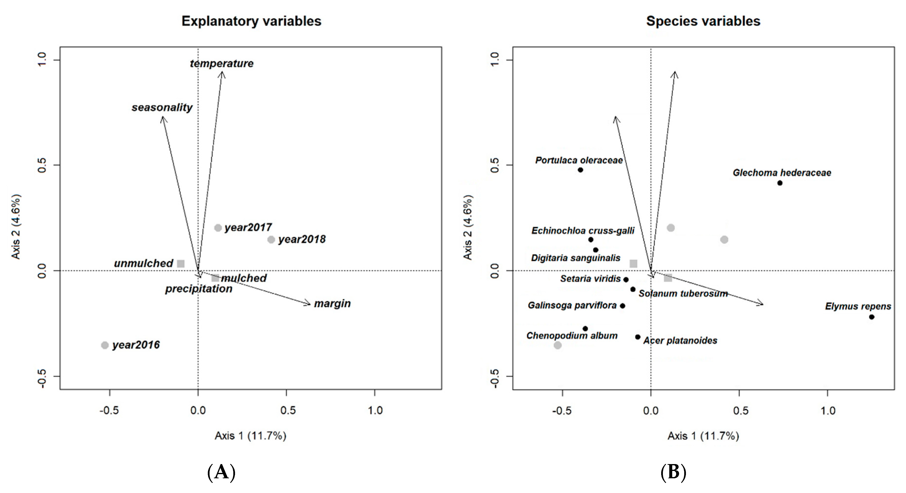
In addition to primary variables of the experiment (mulching and irrigation), we included the following parameters: margin, year, seasonality within year, temperature and precipitation, all with potential influence on germination, as explanatory variables to support the use and versatility of the experimental setting. The model we set up may serve as an indirect tool to prove the impact of mulching on germination. The effect of the bordering vegetation (mown grassland) around the experimental field was included in the model as a ‘margin’ effect, in order to reflect how perennial weeds can invade the marginal microplots.
The model of the open-field survey included the following explanatory variables: mulching (factorial variable; yes or no), irrigation (numeric variable; the total amount of water in mm in three weeks before survey), margin (interval variable; number of sides of microplots directly bordered by the mown grassland margin: 0, 1 or 2), year (factorial variable; 2016, 2017 or 2018), seasonality (interval variable; 1–5, representing the order of weed survey within each year), precipitation (numeric variable; the total amount of rainfall in mm in three weeks before each survey) and temperature (numeric variable; the average of mean daily temperatures in °C of three weeks before each survey).
The model of weed seed bank test included the following explanatory variables: mulching (factorial variable; yes or no), irrigation (factorial variable; yes or no), margin (interval variable; 0, 1, or 2), year (factorial variable; 2017 or 2018).
Both analyses started, with performing a multivariate analysis to determine the average community composition of every field. Then, for every field, we averaged the cover values of weed species across all the four microplots. Cover values were then subjected to a Hellinger transformation [
36] and were examined in a redundancy analysis (RDA), together with management and environmental factors. Following the procedure described by Legendre and Gallagher [
36], this relates species data to explanatory variables more accurately than the canonical correspondence analysis (CCA), even if the species response curves are unimodal (owing to, e.g., long gradients). The number of explanatory variables was reduced by stepwise backward selection using a
p < 0.05 threshold for type I error, which led to a minimal adequate model containing 6 terms (in the case of open-field experiment) and 4 terms (in the case of soil seed bank test). The sole excluded variable was the irrigation in both open-field and soil seed bank test.
As a next step of the multivariate analysis, we assessed gross and net effects of each explanatory variable of the reduced model, according to the methodology of Lososová et al. [
37]. The gross effect of a variable was defined as the variation explained by a ‘univariate’ RDA containing the studied predictor as the only explanatory variable. The net effect, on the other hand, was assessed as the significance of a similar partial RDA (pRDA) with the studied predictor still being the only constraining variable, but all the other variables of the reduced model were also involved as conditioning variables (‘co-variables’), the effect of which was ‘partialled out’ (i.e., removed before the actual RDA). In the case of net effects, model significances were assessed as type I error rates were obtained by permutation tests. There was only one constrained axis in the partial RDAs, except for analyzing year in the case of open-field test, where there were two constrained axes (number of categories—1), and all axes were tested separately [
38].
Based on these results, a common rank of ‘importance’ was established among all explanatory variables according to the R2 adj-values of the net effects of the pRDA models. To demonstrate the responses of the weed species to the individual significant management and environmental factors, in each case, we identified 10 species (with >3 occurrences) that expressed the highest explained variation by the constrained axis in the partial RDA.
To check for the presence of spatial autocorrelation or spatially structured species–environment relationship, we applied spatial partitioning of ordination results [
39]. Having found no significant spatial effects, we followed the analysis without considering spatial position of fields. Intercorrelations of model terms were checked prior to the analysis by calculating variance inflation factors [
40]. Significant variables showed only slight intercorrelations, which do not bias the analysis, the highest GVIF (generalized variance inflation factor) score adjusted by a degree of freedom was 2.51 (in the case of an open-field experiment) and 1.01 (in the case of a soil seed bank test).
In the RDA ordination diagrams of the reduced model, co-ordinates of continuous variables were calculated from their linear constraints, while categorical variables were transformed to ‘dummy’ indicator variables, and these dummies were placed in the ordination space by weighted average calculations.
Both numeric and factorial variables were tested by Analysis of Covariance (ANCOVA) in the case of total weed coverage and weeding time during open-field experiments. In significant cases, explanatory variables were tested by a two-samples T-test, or by a Tukey comparison for factorial variables and by Pearson correlation for numeric variables.
The entire statistical analysis was performed in the R Environment (R Development Core Team, version 3.5.3) using the Vegan and Car add-on packages (vegan 2.5-4 and car 3.0-2).


