

Downscaling Climatic Variables at a River Basin Scale: Statistical Validation and Ensemble Projection under Climate Change Scenarios

 ,
,  and
and
Abstract
:1. Introduction
2. Materials and Methods
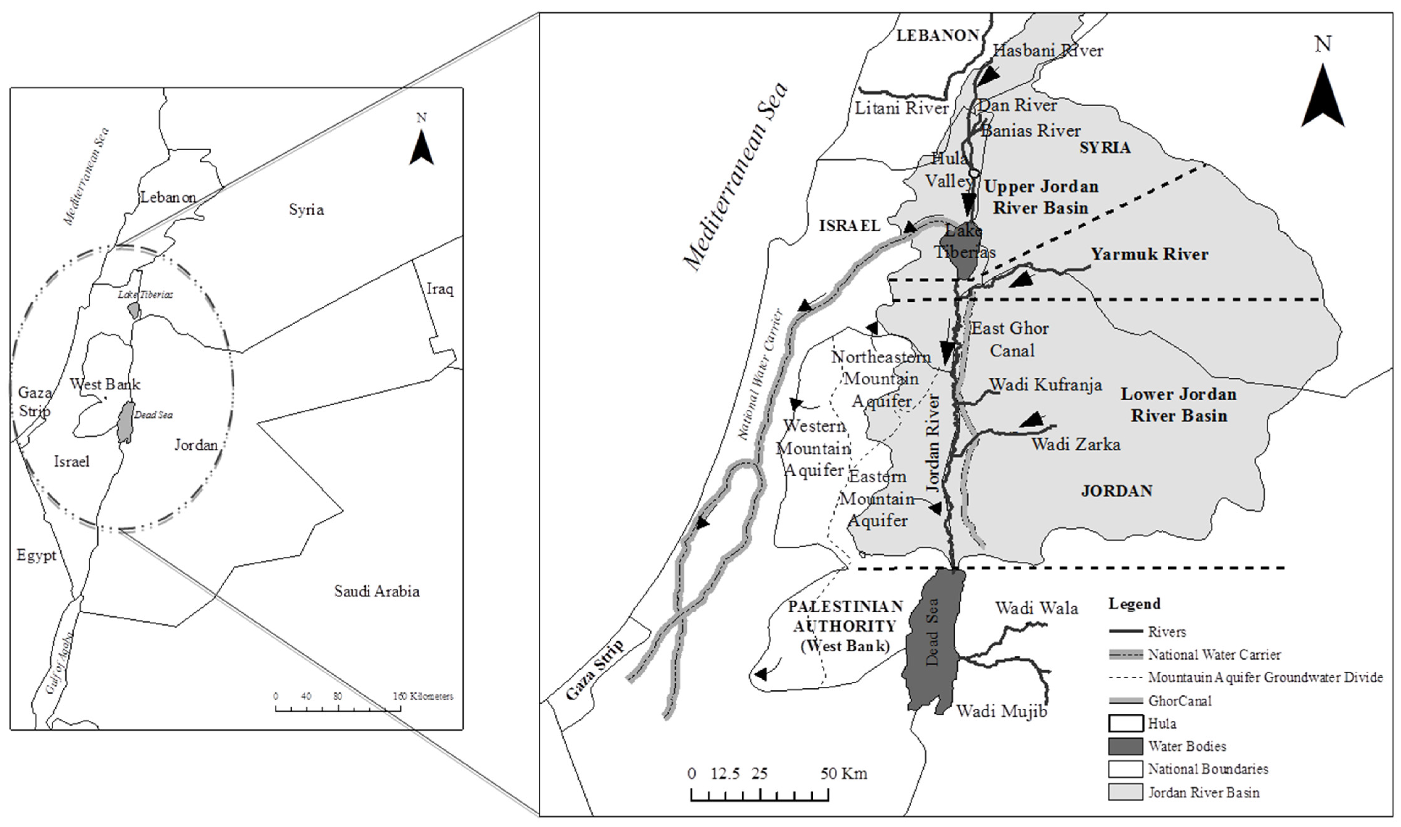
2.1. Study Area and Data
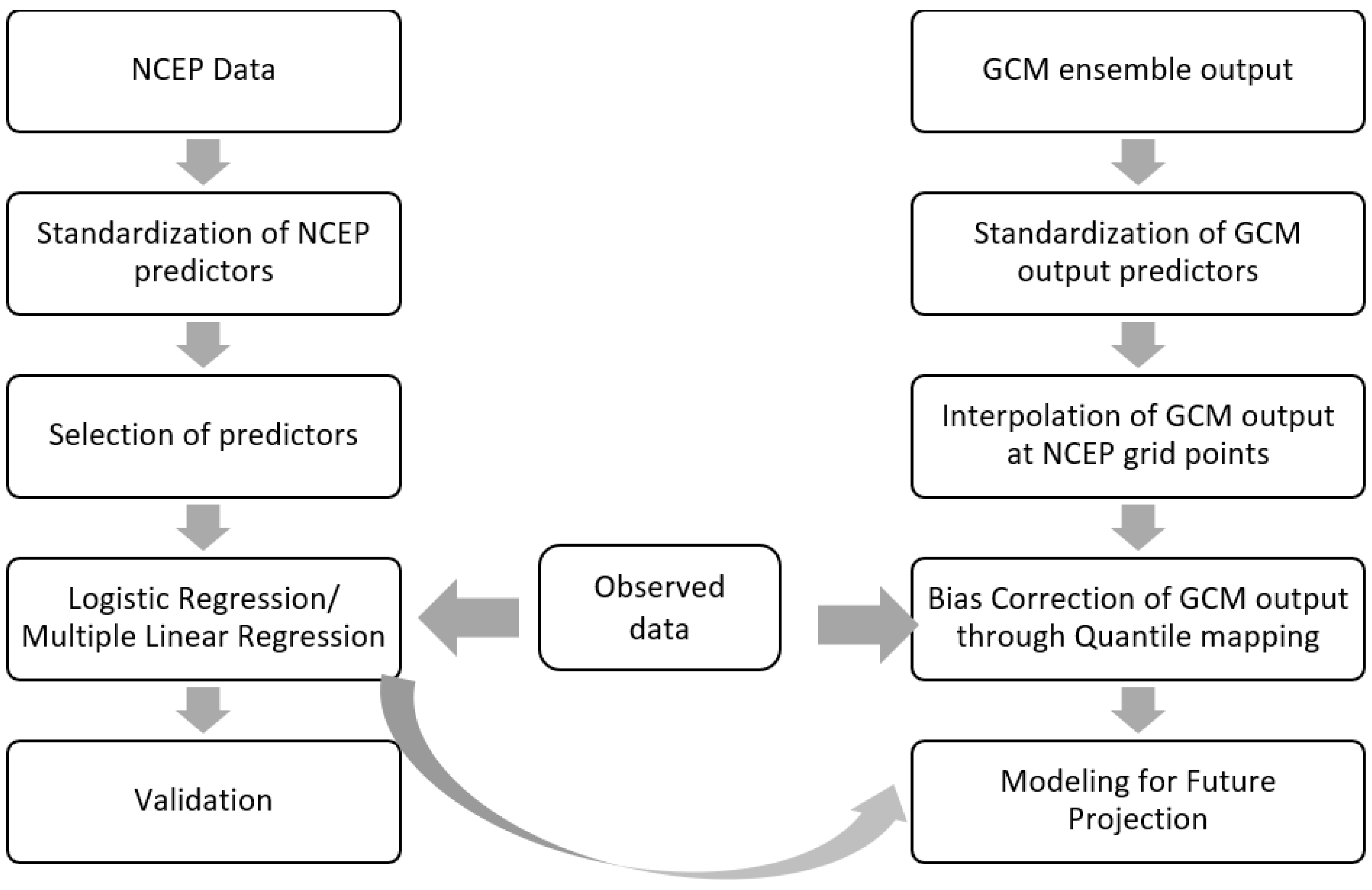
2.2. Re-Gridding and Standardization
2.3. Selection of Predictors
2.4. Downscaling
2.4.1. Logistic Regression
2.4.2. Multiple Linear Regression
2.5. Bias Correction
2.6. Scenario Generation
3. Results
3.1. Selection of Predictors
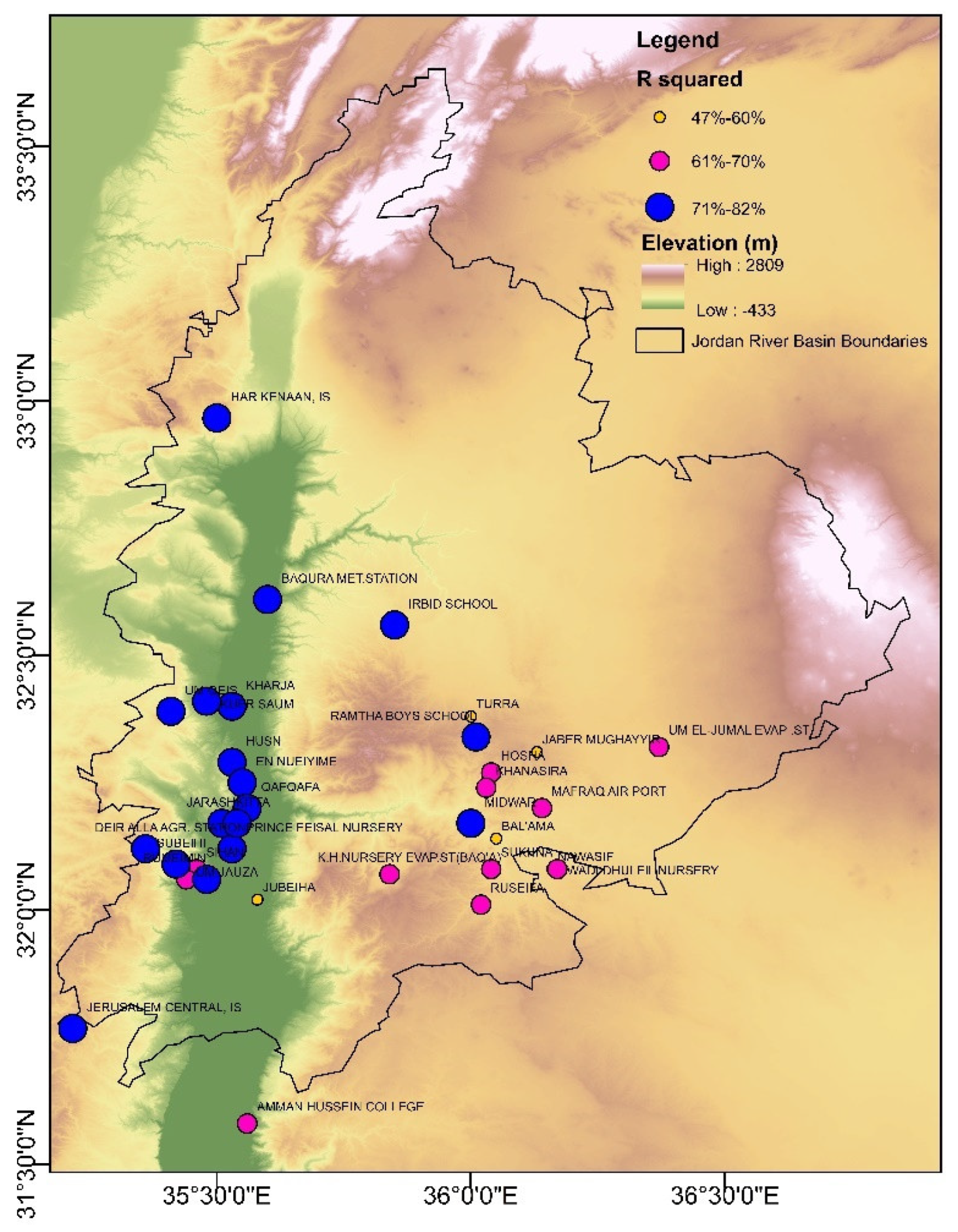
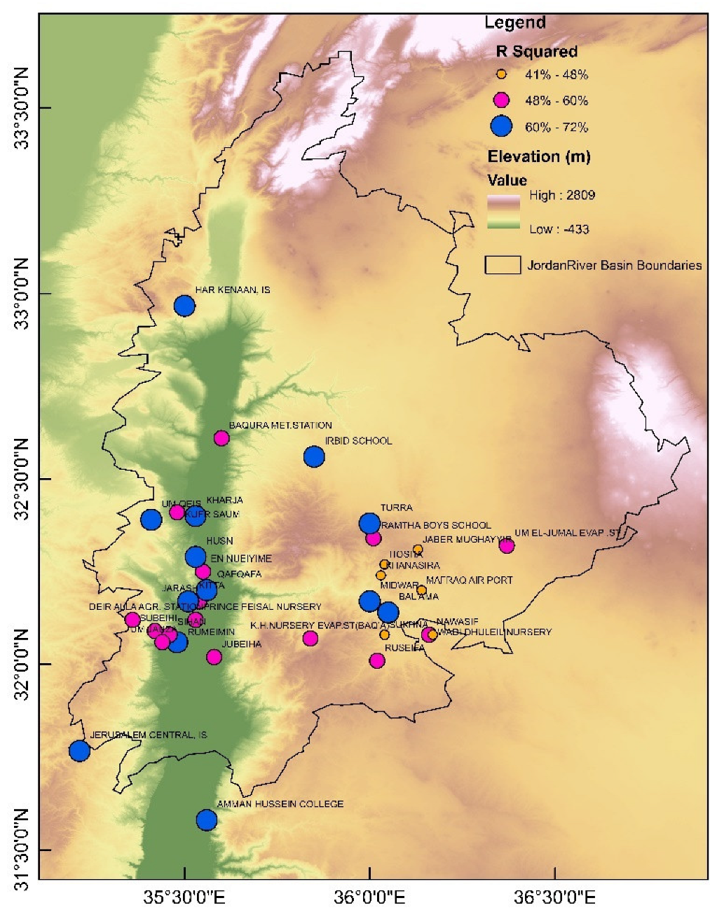
3.2. Downscaling
3.2.1. Precipitation
3.2.2. Temperature
3.3. Bias Correction
3.4. Scenario Generation
4. Discussion
5. Conclusions
Supplementary Materials
Author Contributions
Funding
Data Availability Statement
Conflicts of Interest
References
- Benestad, R.; Hanssen-Bauer, I.; Førland, E.J. An evaluation of statistical models for downscaling precipitation and their ability to capture long-term trends. Int. J. Climatol. 2007, 27, 649–665. [Google Scholar] [CrossRef]
- Intergovernmental Panel on Climate Change (IPCC). The Physical Science Basis. In Climate Change 2013; Contribution of Working Group I to the Fifth Assessment Report of the Intergovernmental Panel on Climate, Change; Stocker, T.F., Qin, D., Plattner, G.K., Tignor, M., Allen, S.K., Boschung, J., Nauels, A., Xia, Y., Bex, V., Midgley, P.M., Eds.; Cambridge University Press: Cambridge, UK, 2013. [Google Scholar]
- Doublas, F.J.; Garcia-Serrano, J.; Lienert, F.; Biescas, A.P.; Rodriguez, L.R.L. Seasonal climate predictability and forecasting: Status and prospects. Wiley Interdiscip. Rev. Clim. Chang. 2013, 4, 245–268. [Google Scholar] [CrossRef]
- Kundu, S.; Khare, D.; Mondal, A. Future projection of rainfall by statistical downscaling method in a part of Central India. In Environment and Earth Observation: Case Studies in India; Hazra, S., Mukhopadhyay, A., Ghosh, A.R., Mitra, D., Dadhwal, V.K., Eds.; Springer International Publishing: Cham, Switzerland, 2017; pp. 57–70. [Google Scholar]
- Xu, C.-Y. From GCMs to river flow: A review of downscaling methods and hydrologic modelling approaches. Prog. Phys. Geogr. 1999, 23, 229–249. [Google Scholar] [CrossRef]
- McGuffie, K.; Henderson-Sellers, A. The Climate Modelling Primer; John Wiley & Sons: Hoboken, NJ, USA, 2014. [Google Scholar]
- Kendon, E.J.; Prein, A.F.; Senior, C.A.; Stirling, A. Challenges and outlook for convection-permitting climate modelling. Philos. Trans. R. Soc. A 2021, 379, 20190547. [Google Scholar] [CrossRef]
- Laprise, R. Regional climate modelling. J. Comput. Phys. 2008, 22, 3641–3666. [Google Scholar] [CrossRef]
- Meehl, G.A.; Stocker, T.F.; Collins, W.; Friedlingstein, P.; Gaye, A.; Gregory, J.; Kitoh, A.; Murphy, J.; Noda, A.; Raper, S.; et al. Global climate projections. In Climate Change 2007: The Physical Science Basis; Solomon, S., Qin, D., Manning, M., Chen, Z., Marquis, M., Averyt, K.B., Tignor, M., Miller, H.L., Eds.; Contribution of Working Group I to the Fourth Assessment Report of the Intergovernmental Panel on Climate Change; Cambridge University Press: Cambridge, UK; New York, NY, USA, 2007; pp. 747–846. [Google Scholar]
- Parry, M.L.; Canziani, O.F.; Palutikof, J.P. Technical Summary. In Climate Change 2007: Impacts, Adaptation and Vulnerability; Parry, M.L., Canziani, O.F., Palutikof, J.P., van der Linden, P.J., Hanson, C.E., Eds.; Contribution of Working Group II to the Fourth Assessment Report of the Intergovernmental Panel on Climate Change; Cambridge University Press: Cambridge, UK, 2007; pp. 23–78. [Google Scholar]
- Dibike, Y.B.; Coulibaly, P. Downscaling Global Climate Model Outputs to Study the Hydrologic Impact of Climate Change Part II: Scenario Simulation and Hydrologic Modeling. In Proceedings of the 6th International Coonfrenece on Hydroinformatics, Singapore, 21–24 June 2004; World Scientific Publishing Company: Singapore, 2005; pp. 1449–1456. [Google Scholar]
- Mearns, L.O.; Giorgi, F.; Whetton, P.; Pabon, D.; Hulme, M.; Lal, M. Guidelines for Use of Climate Scenarios Developed from Regional Climate Model Experiments; IPCC: Geneva, Switzerland, 2003. [Google Scholar]
- Wilby, R.L.; Charles, S.P.; Zorita, E.; Timbal, B.; Whetton, P.; Mearns, L.O. Guidelines for Use of Climate Scenarios Developed from Statistical Downscaling Methods; Intergovernmental Panel on Climate Change Task Group on Data and Scenario Support for Impacts and Climate Analysis; IPCC: Geneva, Switzerland, 2004. [Google Scholar]
- Maraun, D.; Wetterhall, F.; Ireson, A.M.; Chandler, R.E.; Kendon, E.J.; Widmann, M.; Brienen, S.; Rust, H.W.; Sauter, T.; Themeßl, M.; et al. Precipitation downscaling under climate change: Recent developments to bridge the gap between dynamical models and the end user. Rev. Geophys. 2010, 48, RG3003. [Google Scholar] [CrossRef]
- Xue, Y.; Janjic, Z.; Dudhia, J.; Vasic, R.; Sales, F.D. A review on regional dynamical downscaling in intraseasonal to seasonal simulation/prediction and major factors that affect downscaling ability. Atmos. Res. 2014, 147–148, 68–85. [Google Scholar] [CrossRef]
- Daniels, A.E.; Morrison, J.F.; Joyce, L.A.; Crookston, N.L.; Chen; McNulty, S.G. Climate Projections FAQ; General Technical Report RMRS-GTR-277WWW; US Department of Agriculture, Forest Service, Rocky Mountain Research Station: Fort Collins, CO, USA, 2012; 32p. [Google Scholar] [CrossRef]
- Seaby, L.P.; Refsgaard, J.C.; Sonnenborg, T.O.; Stisen, S.; Christensen, J.H.; Jensen, K.H. Assessment of robustness and significance of climate change signals for an ensemble of distribution-based scaled climate projections. J. Hydrol. 2013, 486, 479–493. [Google Scholar] [CrossRef]
- Anandhi, A.; Srinivas, V.V.; Nanjundiah, R.S.; Kumar, D.N. Downscaling precipitation to river basin in India for IPCC SRES scenarios using support vector machine. Int. J. Climatol. 2008, 28, 401–420. [Google Scholar] [CrossRef]
- Hobeichi, S.; Nishant, N.; Shao, Y.; Abramowitz, G.; Pitman, A.; Sherwood, S.; Bishop, C.; Green, S. Using machine learning to cut the cost of dynamical downscaling. Earth’s Future 2023, 11, e2022EF003291. [Google Scholar] [CrossRef]
- Choi, B.; Bergés, M.; Bou-Zeid, E.; Pozzi, M. Short-term probabilistic forecasting of meso-scale near-surface urban temperature fields. Environ. Model. Softw. 2021, 145, 105189. [Google Scholar] [CrossRef]
- Frías, M.D.; Zorita, E.; Fernández, J.; Rodríguez-Puebla, C. Testing statistical downscaling methods in simulated climates. Geophys. Res. Lett. 2006, 33, L19807. [Google Scholar] [CrossRef]
- Giorgi, F.; Whetton, P.H.; Jones, R.G.; Christensen, J.H.; Mearns, L.O.; Hewitson, B.; von Storch, H.; Francisco, R.; Jack, C. Emerging patterns of simulated regional climatic changes for the 21st century due to anthropogenic forcings. Geophys. Res. Lett. 2001, 28, 3317–3320. [Google Scholar] [CrossRef]
- Gutiérrez, J.M.; San-Martín, D.; Brands, S.; Manzanas, R.; Herrera, S. Reassessing statistical downscaling techniques for their robust application under climate change conditions. J. Clim. 2013, 26, 171–188. [Google Scholar] [CrossRef]
- Wilby, R.L.; Wigley, T.M.L.; Conway, D.; Jones, P.D.; Hewitson, B.C.; Main, J.; Wilks, D.S. Statistical downscaling of general circulation model output: A comparison of methods. Water Resour. Res. 1998, 34, 2995–3008. [Google Scholar] [CrossRef]
- Adem, A.; Melesse, A.; Tilahun, S.; Setegn, S.G.; Ayana, E.; Wale, A.; Assefa, T. Climate change projections in the Upper Gilgel Abay river catchment, Blue Nile basin Ethiopia. In Nile River Basin: Ecohydrological Challenges, Climate Change and Hydropolitic; Melesse, A., Abtew, W., Setegn, S.G., Eds.; Springer Science & Business Media: Berlin/Heidelberg, Germany, 2014; pp. 363–388. [Google Scholar]
- Zorita, E.; Von Storch, H. The analog method as a simple statistical downscaling technique: Comparison with more complicated methods. J. Clim. 1999, 12, 2474–2489. [Google Scholar] [CrossRef]
- Flaounas, E.; Drobins, P.; Vrac, M.; Bastin, S.; Lebeaupin-Brossier, C.; Stéfanon, M.; Borga, M.; Calvet, J.-C. Precipitation and temperature space-time variability and extremes in the Mediterranean region: Evaluation of dynamical and statistical downscaling methods. Clim. Dyn. 2013, 40, 2687–2705. [Google Scholar] [CrossRef]
- Fowler, H.J.; Blenkin, S.; Tebaldi, C. Linking climate change modelling to impacts studies: Recent advances in downscaling techniques for hydrological modelling. Int. J. Climatol. 2007, 27, 1547–1578. [Google Scholar] [CrossRef]
- Trzaska, S.; Schnarr, E. A Review of Downscaling Methods for Climate Change Projections; United States Agency for International Development by Tetra Tech ARD: Washington, DC, USA, 2014; pp. 1–42. [Google Scholar]
- Maraun, D.; Widmann, M.; Gutiérrez, J.M.; Kotlarski, S.; Chandler, R.E.; Hertig, E.; Wibig, J.; Huth, R.; Wilcke, R.A.I. VALUE: A framework to validate downscaling approaches for climate change studies. Earth’s Future 2015, 3, 1–14. [Google Scholar] [CrossRef]
- Hall, A. Projecting regional change. Science 2014, 346, 1461–1462. [Google Scholar] [CrossRef]
- Baño-Medina, J.; Manzanas, R.; Gutiérrez, J.M. Configuration and intercomparison of deep learning neural models for statistical downscaling. Geosci. Model Dev. 2020, 13, 2109–2124. [Google Scholar] [CrossRef]
- Nasseri, M.; Tavakol-Davani, H.; Zahraie, B. Performance assessment of different data mining methods in statistical downscaling of daily precipitation. J. Hydrol. 2013, 492, 1–14. [Google Scholar] [CrossRef]
- Khalili, M.; Brissette, F.; Leconte, R. Stochastic multi-site generation of daily weather data. Stoch. Environ. Res. Risk Assess. 2008, 23, 837–849. [Google Scholar] [CrossRef]
- Wilby, R.L.; Troni, J.; Biot, Y.; Tedd, L.; Hewitson, B.C.; Smith, D.G.; Sutton, R.T. A review of climate risk information for adaptation and development planning. Int. J. Climatol. 2009, 29, 1193–1215. [Google Scholar] [CrossRef]
- Wilks, D.S.; Wilby, R.L. The weather generation game: A review of stochastic weather models. Prog. Phys. Geogr. 1999, 23, 329–357. [Google Scholar] [CrossRef]
- Chu, J.T.; Xia, J.; Xu, C.; Singh, V.P. Statistical downscaling of daily mean temperature, pan evaporation and precipitation for climate change scenarios in Haihe River, China. Theor. Appl. Climatol. 2009, 99, 149–161. [Google Scholar] [CrossRef]
- Gagnon, S.; Singh, B.; Rousselle, J.; Roy, L. An application of the statistical downscaling model (SDSM) to simulate climatic data for streamflow modelling in Québec. Can. Water Resour. J. 2005, 30, 297–314. [Google Scholar] [CrossRef]
- Huang, J.; Zhang, J.; Zhang, Z.; Xu, C.; Wang, B.; Yao, J. Estimation of future precipitation change in the Yangtze River basin by using statistical downscaling method. Stoch. Environ. Res. Risk Assess. 2010, 25, 781–792. [Google Scholar] [CrossRef]
- Mahmood, R.; Babel, M.S. Future changes in extreme temperature events using the statistical downscaling model (SDSM) in the trans-boundary region of the Jhelum river basin. Weather. Clim. Extrem. 2014, 5–6, 56–66. [Google Scholar] [CrossRef]
- Wang, X.; Yang, T.; Shao, Q.; Acharya, K.; Wang, W.; Yu, Z. Statistical downscaling of extremes of precipitation and temperature and construction of their future scenarios in an elevated and cold zone. Stoch. Environ. Res. Risk Assess. 2012, 26, 405–418. [Google Scholar] [CrossRef]
- Wilby, R.; Dawson, C.; Barrow, E. SDSM—A decision support tool for the assessment of regional climate change impacts. Environ. Model. Softw. 2002, 17, 145–157. [Google Scholar] [CrossRef]
- Lutz, K.; Jacobeit, J.; Philipp, A.; Seubert, S.; Kunstmann, H.; Laux, P. Comparison and evaluation of statistical downscaling techniques for station-based precipitation in the Middle East. Int. J. Climatol. 2012, 32, 1579–1595. [Google Scholar] [CrossRef]
- Khan, M.S.; Coulibaly, P.; Dibike, Y. Uncertainty analysis of statistical downscaling methods. J. Hydrol. 2006, 319, 357–382. [Google Scholar] [CrossRef]
- Bou-Zeid, E.; El-Fadel, M. Climate change and water resources in Lebanon and the Middle East. J. Water Resour. Plan. Manag. 2002, 128, 343–355. [Google Scholar] [CrossRef]
- Gunkel, A.; Lange, J. Water scarcity, data scarcity and the Budyko curve—An application in the Lower Jordan River Basin. J. Hydrol. Reg. Stud. 2017, 12, 136–149. [Google Scholar] [CrossRef]
- Atwi, M.; Chóliz, J.S. A negotiated solution for the Jordan Basin. J. Oper. Res. Soc. 2010, 62, 81–91. [Google Scholar] [CrossRef]
- Comair, G.F.; Mckinney, D.C.; Siegel, D. Hydrology of the Jordan river basin: Watershed delineation, precipitation and evapotranspiration. Water Resour. Manag. 2012, 26, 4281–4293. [Google Scholar] [CrossRef]
- Smiatek, G.; Kunstmann, H.; Heckl, A. High-resolution climate change simulations for the Jordan River area. J. Geophys. Res. 2011, 116, D16111. [Google Scholar] [CrossRef]
- El-Fadel, M.; Maroun, R. Future water resources management for the Middle East. J. Soc. Aff. 2003, 20, 51–79. [Google Scholar]
- Alpert, P.; Krichak, S.O.; Shafir, H.; Hiam, D.; Osetins, I. Climatic trends to extremes employing regional modeling and statistical interpretation over the E. Mediterranean. Glob. Planet. Change 2008, 63, 163–170. [Google Scholar] [CrossRef]
- Kundzewicz, Z.W.; Mata, L.J.; Arnell, N.W.; Döll, P.; Kabat, P.; Jiménez, B.; Miller, K.; Oki, T.; Sen, Z.; Shiklomanov, I.A. Freshwater resources and their management. In Climate Change 2007: Impacts, Adaptation and Vulnerability; Parry, M.L., Canziani, O.F., Palutikof, J.P., van der Linden, P.J., Hanson, C.E., Eds.; Contribution of Working Group II to the Fourth Assessment Report of the Intergovernmental Panel on Climate Change; Cambridge University Press: Cambridge, UK, 2007; pp. 173–210. [Google Scholar]
- Samuels, R.; Rimmer, A.; Hartmann, A.; Krichak, S.; Alpert, P. Climate change impacts on Jordan river flow: Downscaling application from a regional climate model. J. Hydrometeorol. 2010, 11, 860–879. [Google Scholar] [CrossRef]
- Kalnay, E.; Kanamitsu, M.; Kristler, R.; Collins, W.; Deaven, D.; Gandin, L.; Iredell, M.; Saha, S.; White, G.; Woollen, J.; et al. The NCEP/NCAR 40-year reanalysis project. Bull. Am. Meteorol. Soc. 1996, 77, 437–472. [Google Scholar] [CrossRef]
- Cannon, A.J.; Whitfield, P.H. Downscaling recent streamflow conditions in British Columbia, Canada using ensemble neural network models. J. Hydrol. 2002, 259, 136–151. [Google Scholar] [CrossRef]
- Taylor, K.E.; Stouffer, R.J.; Meehl, G.A. An overview of CMIP5 and the experiment design. Bull. Am. Meteorol. Soc. 2012, 93, 485–498. [Google Scholar] [CrossRef]
- Clarke, L.; Edmond, J.; Jacobs, H.; Pitcher, H.; Reilly, J.; Richels, R. CCSP Synthesis and Assessment Product 2.1, Part A: Scenarios of Greenhouse Gas Emissions and Atmospheric Concentrations; U.S. Government Printing Office: Washington, DC, USA, 2007. [Google Scholar]
- Sachindra, D.; Huang, F.; Barton, A.; Perera, B. Statistical downscaling of general circulation model outputs to precipitation-part 2: Bias-correction and future projections. Int. J. Climatol. 2014, 34, 3282–3303. [Google Scholar] [CrossRef]
- Dubrovský, M.; Hayes, M.; Duce, P.; Trnka, M.; Svoboda, M.; Zara, P. Multi-GCM projections of future drought and climate variability indicators for the Mediterranean region. Reg. Environ. Change 2013, 14, 1907–1919. [Google Scholar] [CrossRef]
- United Nations Economic & Social Commission for Western Asia (ESCWA). Arab Climate Change Assessment Report—Main Report; E/ESCWA/SDPD/2017/RICCAR/Report; ESCWA: Beirut, Lebanon, 2017. [Google Scholar]
- Chen, F.W.; Liu, C.W. Estimation of the spatial rainfall distribution using inverse distance weighting (IDW) in the middle of Taiwan. Paddy Water Environ. 2012, 10, 209–222. [Google Scholar] [CrossRef]
- Bedient, P.B.; Huber, W.C. Hydrology and Floodplain Analysis; Addison-Wesley: New York, NY, USA, 1992. [Google Scholar]
- Burrough, P.A.; McDonnell, R.A.; Lloyd, C.D. Principles of Geographical Information Systems; Oxford University Press: Oxford, MA, USA, 2015. [Google Scholar]
- Goovaerts, P. Geostatistical approaches for incorporating elevation into the spatial interpolation of rainfall. J. Hydrol. 2000, 228, 113–129. [Google Scholar] [CrossRef]
- Li, J.; Heap, A.D. A Review of Spatial Interpolation Methods for Environmental Scientists; Geoscience Australia: Symonston, ACT, Australia, 2008. [Google Scholar]
- Zhu, H.Y.; Jia, S. Uncertainty in the spatial interpolation of rainfall data. Prog. Geogr. 2004, 23, 34–42. [Google Scholar]
- Lin, X.S.; Yu, Q. Study on the spatial interpolation of agroclimatic resources in Chongqing. J. Anhui Agric. 2008, 36, 13431–13463. [Google Scholar]
- Chiew, F.H.; McMahon, T.A. Global ENSO-streamflow teleconnection, streamflow forecasting and interannual variability. Hydrol. Sci. J. 2002, 47, 505–522. [Google Scholar] [CrossRef]
- Mpelasoka, F.S.; Chiew, F.H. Influence of rainfall scenario construction methods on runoff projections. J. Hydrometeorol. 2009, 10, 1168–1183. [Google Scholar] [CrossRef]
- Ines, A.V.; Hansen, J.W. Bias correction of daily GCM rainfall for crop simulation studies. Agric. For. Meteorol. 2006, 138, 44–53. [Google Scholar] [CrossRef]
- Li, H.; Sheffield, J.; Wood, E.F. Bias correction of monthly precipitation and temperature fields from Intergovernmental Panel on Climate Change AR4 models using equidistant quantile matching. J. Geophys. Res. Atmos. 2010, 115, D10101. [Google Scholar] [CrossRef]
- Piani, C.; Haerter, J.O.; Coppola, E. Statistical bias correction for daily precipitation in regional climate models over Europe. Theor. Appl. Climatol. 2010, 99, 187–192. [Google Scholar] [CrossRef]
- Wood, A.W.; Leung, L.R.; Sridhar, V.; Lettenmaier, D.P. Hydrologic implications of dynamical and statistical approaches to downscaling climate model outputs. Clim. Chang. 2004, 62, 189–216. [Google Scholar] [CrossRef]
- Rogerson, P.A. A statistical method for the detection of geographic clustering. Geogr. Anal. 2010, 33, 215–227. [Google Scholar] [CrossRef]
- Haylock, M.R.; Cawley, G.C.; Harpham, C.; Wilby, R.L.; Goodess, C.M. Downscaling heavy precipitation over the United Kingdom: A comparison of dynamical and statistical methods and their future scenarios. Int. J. Climatol. 2006, 26, 1397–1415. [Google Scholar] [CrossRef]
- Nabeel, A.; Athar, H. Classification of precipitation regimes in Pakistan using wet and dry spells. Int. J. Climatol. 2018, 38, 2462–2477. [Google Scholar] [CrossRef]
- McFadden, D. Conditional Logit Analysis of Qualitative Choice Behavior; Institute of Urban and Regional Development, University of California: Berkeley, CA, USA, 1973. [Google Scholar]
- R Core Team. R: A Language and Environment for Statistical Computing; R Foundation for Statistical Computing: Vienna, Austria, 2017; Available online: https://www.R-project.org/ (accessed on 13 June 2019).
- Helsel, D.R.; Hirsch, R.M. Statistical Methods in Water Resources Techniques of Water Resources Investigation; U.S. Geological Survey: Reston, VA, USA, 2002; Chapter A3, Book 4. [Google Scholar]
- Chen, J.; Brissette, F.P.; Chaumont, D.; Braun, M. Finding appropriate bias correction methods in downscaling precipitation for hydrologic impact studies over North America. Water Resour. Res. 2013, 49, 4187–4205. [Google Scholar] [CrossRef]
- Teutschbein, C.; Seibert, J. Bias correction of regional climate model simulations for hydrological climate-change impact studies: Review and evaluation of different methods. J. Hydrol. 2012, 456–457, 12–29. [Google Scholar] [CrossRef]
- Piani, C.; Weedon, G.; Best Gomes, M.S.; Viterbo, P.; Hagemann, S.; Haerter, J. Statistical bias correction of global simulated daily precipitation and temperature for the application of hydrological models. J. Hydrol. 2010, 395, 199–215. [Google Scholar] [CrossRef]
- Ghosh, S.; Mujumdar, P.P. Statistical downscaling of GCM simulations to streamflow using relevance vector machine. Adv. Water Resour. 2008, 31, 132–146. [Google Scholar] [CrossRef]
- Gulacha, M.M.; Mulungu, D.M.M. Generation of climate change scenarios for precipitation and temperature at local scales using SDSM in Wami-Ruvu River Basin Tanzania. Phys. Chem. Earth Parts A/B/C 2017, 100, 62–72. [Google Scholar] [CrossRef]
- Sachindra, D.; Huang, F.; Barton, A.; Perera, B. Least square support vector and multi-linear regression for statistically downscaling general circulation model outputs to catchment stream flows. Int. J. Climatol. 2013, 33, 1087–1106. [Google Scholar] [CrossRef]
- Souvignet, M.; Gaese, H.; Ribbe, L.; Kretschmer, N.; Oyarzún, R. Statistical downscaling of precipitation and temperature in north-central Chile: An assessment of possible climate change impacts in an arid Andean watershed. Hydrol. Sci. J. 2010, 55, 41–57. [Google Scholar] [CrossRef]
- Aksornsingchai, P.; Srinilta, C. Statistical downscaling for rainfall and temperature prediction in Thailand. In Proceedings of the International Multiconference of Engineers and Computer Scientists, Hong Kong, China, 16–18 March 2011. [Google Scholar]
- Samadi, S.; Carbone, G.; Mahdavi, M.; Sharifi, F.; Bihamta, M. Statistical downscaling of river runoff in a semi-arid catchment. Water Resour. Manag. 2013, 27, 117–136. [Google Scholar] [CrossRef]
- Hertig, E.; Jacobeit, J. Assessments of Mediterranean Precipitation Changes for the 21st Century Using Statistical Downscaling Techniques. Int. J. Climatol. 2008, 28, 1025–1045. [Google Scholar] [CrossRef]
- El-Samra, R.; Bou-Zeid, E.; Bangalath, H.K.; Stenchikov, G.; El-Fadel, M. Future intensification of hydro-meteorological extremes: Downscaling using the Weather Research and Forecasting model. Clim. Dyn. 2017, 49, 3765–3785. [Google Scholar] [CrossRef]
- Huth, R. Statistical downscaling of daily temperature in central Europe. J. Clim. 2002, 15, 1731–1742. [Google Scholar] [CrossRef]
- Gachon, P. FINAL REPORT “A First Evaluation of the Strength and Weaknesses of Statistical Downscaling Methods for Simulating Extremes over Various Regions of Eastern Canada”; Meteorological Service of Canada: Toronto, ON, Canada, 2005. [Google Scholar]
- Tavakol-Davani, H.; Nasseri, M.; Zahraie, B. Improved statistical downscaling of daily precipitation using SDSM platform and data-mining methods. Int. J. Climatol. 2013, 33, 2561–2578. [Google Scholar] [CrossRef]
- Pomee, M.S.; Hertig, E. Temperature Projections over the Indus River Basin of Pakistan Using Statistical Downscaling. ATM 2021, 12, 195. [Google Scholar] [CrossRef]
- Araya-Osses, D.; Casanueva, A.; Román-Figueroa, C.; Uribe, J.M.; Paneque, M. Climate change projections of temperature and precipitation in Chile based on statistical downscaling. Clim. Dyn. 2020, 54, 4309–4330. [Google Scholar] [CrossRef]
- Phuong, D.N.; Duong, T.Q.; Liem, N.D.; Tram, V.N.; Cuong, D.K.; Loi, N.K. Projections of Future Climate Change in the Vu Gia Thu Bon River Basin, Vietnam by Using Statistical Down Scaling Model (SDSM). Water 2020, 12, 755. [Google Scholar] [CrossRef]
- Mukhtar, M.; Qasim, M. Future predictions of precipitation and temperature in Iraq using the statistical downscaling model. Arab. J. Geosci. 2019, 12, 25. [Google Scholar] [CrossRef]
- Sachindra, D.; Ahmed, K.; Rashid, M.; Shahid, S.; Perera, B. Statistical downscaling of precipitation using machine learning techniques. Atmos. Res. 2018, 212, 240–258. [Google Scholar] [CrossRef]
- Tahir, T.; Hashim, A.M.; Yusof, K.W. Statistical downscaling of rainfall under transitional climate in Limbang River Basin by using SDSM. IOP Conference Series: Earth Environ. Sci. 2018, 140, 012037. [Google Scholar] [CrossRef]
- Rashid, M.M.; Beecham, S.; Chowdhury, R.K. Statistical downscaling of CMIP5 outputs for projecting future changes in rainfall in the Onkaparinga catchment. Sci. Total Environ. 2015, 530–531, 171–182. [Google Scholar] [CrossRef]
- Beecham, S.; Rashid, M.; Chowdhury, R.K. Statistical downscaling of multi-site daily rainfall in a South Australian catchment using a Generalized Linear Model. Int. J. Climatol. 2014, 34, 3654–3670. [Google Scholar] [CrossRef]
- Goly, A.; Teegavarapu, R.S.V.; Mondal, A. Development and evaluation of statistical downscaling models for monthly precipitation. EI 2014, 18, 1–28. [Google Scholar] [CrossRef]
- Mishra, P.K.; Khare, D.; Mondal, A.; Kundu, S. Multiple linear regression based statistical downscaling of daily precipitation in a canal command. In limate Change and Biodiversity Advances in Geographical and Environmental Sciences; Singh, M., Sngh, R., Hassan, M., Eds.; Springer: Tokyo, Japan, 2014; pp. 73–83. [Google Scholar]
- Pervez, M.S.; Henebry, G.M. Projections of the Ganges–Brahmaputra precipitation—Downscaled from GCM predictors. J. Hydrol. 2014, 517, 120–134. [Google Scholar] [CrossRef]
- Jeong, D.; Hilaire, A.S.; Ouarda, T.; Gachon, P. Multisite statistical downscaling model for daily precipitation combined by multivariate multiple linear regression and stochastic weather generator. Clim. Change 2012, 114, 567–591. [Google Scholar] [CrossRef]
- Meenu, R.; Rehana, S.; Mujumdar, P.P. Assessment of hydrologic impacts of climate change in Tunga–Bhadra river basin, India with HEC-HMS and SDSM. Hydrol. Process 2012, 27, 1572–1589. [Google Scholar] [CrossRef]
- Brands, S.; Taboada, J.J.; Cofiño, A.S.; Sauter, T.; Schneider, C. Statistical downscaling of daily temperatures in the NW Iberian Peninsula from global climate models: Validation and future scenarios. Clim. Res. 2011, 48, 163–176. [Google Scholar] [CrossRef]
- Fistikoglu, O.; Okkan, U. Statistical downscaling of monthly precipitation using NCEP/NCAR reanalysis data for Tahtali river basin in Turkey. J. Hydrol. 2011, 16, 157–164. [Google Scholar] [CrossRef]
- Raje, D.; Mujumdar, P.P. A comparison of three methods for downscaling daily precipitation in the Punjab region. Hydrol. Process 2011, 25, 3575–3589. [Google Scholar] [CrossRef]
- Chen, S.T.; Yu, P.S.; Tang, Y.H. Statistical downscaling of daily precipitation using support vector machines and multivariate analysis. J. Hydrol. 2010, 385, 13–22. [Google Scholar] [CrossRef]
- Hessami, M.; Gachon, P.; Ouarda, T.B.J.; St-Hilaire, A. Automated regression-based statistical downscaling tool. Environ. Model. Softw. 2008, 23, 813–834. [Google Scholar] [CrossRef]
- Pharasi, S. Development of Statistical Downscaling Methods for the Daily Precipitation Process at a Local Site. Master’s Thesis, Department of Civil Engineering and Applied Mechanics, McGill University, Montreal, QC, Canada, 2006. [Google Scholar]
- Harpham, C.; Wilby, R.L. Multi-site downscaling of heavy daily precipitation occurrence and amounts. J. Hydrol. 2005, 312, 235–255. [Google Scholar] [CrossRef]


| Method | Description | Drawbacks | Examples |
|---|---|---|---|
| Weather classification |
| Subjectivity in creating classification states | Principal components, neural networks such as radial basis function (RBF), multilayer perceptron (MLP), analog and fuzzy c-mean clustering |
| Regression |
| Variance underestimation, especially of daily precipitation, because of the non-normality of the process | Examples: multiple linear regression (MLR), positive coefficient regression (PCR), principal component regression (PCR), stepwise regression (SR), and canonical correlation analysis (CCA) |
| Weather generators |
| Examples: K-nearest neighbor (KNN), Markov chains, conditional random fields (CRF) and Gamma distribution are examples of weather generator methods |
| Station Name | Latitude (°) | Longitude (°) | Elevation (m) | Source | Variable | Data Availability | Country |
|---|---|---|---|---|---|---|---|
| Amman Hussein College | 31.58 | 35.56 | 834 | JMD | P | January 2000–March 2012 | JO |
| Bal’ama | 32.14 | 36.05 | 695 | JMD | P | January 2000–March 2012 | JO |
| Baqura Met. Station | 32.61 | 35.60 | −227 | JMD | P | January 1981–April 2009 | JO |
| Damascus International | 33.41 | 36.52 | 616 | NCDC | T | January 1981–December 2017 | SYR |
| Deir Alla Agr. Station | 32.12 | 35.36 | −224 | JMD | P | January 2000–March 2012 | JO |
| En Nueiyime | 32.25 | 35.55 | 748 | JMD | P | January 1981–April 2009 | JO |
| Ghor Safi | 31.03 | 35.47 | −350 | NCDC | T | Jul 1983–December 2017 | JO |
| H4 Airbase | 32.54 | 38.20 | 686 | NCDC | T | January 1981–December 2017 | JO |
| Har Kenaan | 32.97 | 35.50 | 934 | NCDC | P, T | January 1981–December 2017 | IS |
| Hosha | 32.27 | 36.04 | 589 | JMD | P | January 1981–April 2009 | JO |
| Husn | 32.29 | 35.53 | 637 | JMD | P | January 1981–April 2009 | JO |
| Irbid School | 32.56 | 35.85 | 616 | JMD | P | January 1981–April 2009 | JO |
| Jaber Mughayyir | 32.31 | 36.13 | 571 | JMD | P | January 1981–April 2009 | JO |
| Jarash | 32.17- | 35.54 | 585 | JMD | P | January 2000–March 2012 | JO |
| Jerusalem Central | 31.77 | 35.22 | 815 | NCDC | P, T | 1981–2014/1981–1999 | IS |
| Jubeiha | 32.02 | 35.58 | 980 | JMD | P | January 2000–March 2012 | JO |
| K. H. Nursery Evap.St(Baq’a) | 32.07 | 35.84 | 950 | JMD | P | January 2000–March 2012 | JO |
| Khanasira | 32.24 | 36.03 | 810 | JMD | P | January 1981–April 2009 | JO |
| Kharja | 32.40 | 35.53 | 441 | JMD | P | January 1981–April 2009 | JO |
| King Hussein | 32.36 | 36.26 | 683 | NCDC | T | January 1983–December 2017 | JO |
| Kitta | 32.17 | 35.51 | 665 | JMD | P | January 2000–March 2012 | JO |
| Kufr Saum | 32.41 | 35.48 | 423 | JMD | P | January 1981–April 2009 | JO |
| Ma An | 30.17 | 35.78 | 1069 | NCDC | T | January 1981–December 2017 | JO |
| Mafraq Airport | 32.20 | 36.14 | 667 | JMD | P | January 1981–April 2009 | JO |
| Midwar | 32.17 | 36.00 | 760 | JMD | P | January 2000–March 2012 | JO |
| Nawasif | 32.08 | 36.16 | 590 | JMD | P | January 2000–March 2012 | JO |
| Prince Feisal Nursery | 32.12 | 35.53 | 300 | JMD | P | January 2000–March 2012 | JO |
| Prince Hasan | 32.16 | 37.15 | 677 | NCDC | T | January 1981–December 2017 | JO |
| Qafqafa | 32.20 | 35.56 | 930 | JMD | P | January 2000–March 2012 | JO |
| Beirut Airport | 33.82 | 35.49 | 27 | NCDC | T | January 1981–December 2017 | LB |
| Ramtha Boys School | 32.34 | 36.01 | 513 | JMD | P | January 1981–April 2009 | JO |
| Rumeimin | 32.06 | 35.48 | 675 | JMD | P | January 2000–March 2012 | JO |
| Ruseifa | 32.01 | 36.02 | 655 | JMD | P | January 2000–March 2012 | JO |
| Sihan | 32.08 | 35.46 | 495 | JMD | P | January 2000–March 2012 | JO |
| Subeihi | 32.09 | 35.42 | 500 | JMD | P | January 2000–March 2012 | JO |
| Sukhna | 32.08 | 36.04 | 500 | JMD | P | January 2000–March 2012 | JO |
| Turra | 32.38 | 36.00 | 446 | JMD | P | January 1981–April 2009 | JO |
| Um El-Jumal Evap .St | 32.32 | 36.37 | 680 | JMD | P | January 2000–March 2012 | JO |
| Um Jauza | 32.06 | 35.44 | 860 | JMD | P | January 1981–March 2012 | JO |
| Um Qeis | 32.39 | 35.41 | 351 | JMD | P | January 1981–April 2009 | JO |
| Wadi Dhuleil Nursery | 32.08 | 36.17 | 575 | JMD | P | January 2000–March 2012 | JO |
| Model Name | Institution | Atmospheric Grid Resolution | Scenario | Dates | |
|---|---|---|---|---|---|
| Latitude | Longitude | ||||
| CanESM2 | Canadian Centre for Climate Modeling and Analysis | 2.7906° | 2.8125° | Historical | 1981–2005 |
| RCP4.5 | 2006–2050 | ||||
| RCP8.5 | 2006–2050 | ||||
| GFDL-ESM2M | National Oceanic and Atmospheric Administration (NOAA) Geophysical Fluid Dynamics Laboratory | 2.0225° | 2.5° | Historical | 1981–2005 |
| RCP4.5 | 2006–2050 | ||||
| RCP8.5 | 2006–2050 | ||||
| HadGEM-CC | Met Office Hadley Centre | 1.25° | 1.875° | Historical | 1981–2005 |
| RCP4.5 | 2006–2050 | ||||
| RCP8.5 | 2006–2050 | ||||
| Predictor | Abbreviation |
|---|---|
| Temperature at 2 m | Temp2m |
| Pressure | Pressure |
| U wind component (East/West) at 500 pressure level | UWND.500 |
| U wind component (East/West) at 1000 pressure level | UWND.1000 |
| V wind component (North/South) at 500 pressure level | VWND.500 |
| V wind component (North/South) at 1000 pressure level | VWND.1000 |
| Relative humidity at 500 pressure level | RHUM.500 |
| Relative humidity at 1000 pressure level | RHUM.1000 |
| Specific humidity at 500 pressure level | SHUM.500 |
| Specific humidity at 1000 pressure level | SHUM.1000 |
| Geopotential height at 500 mb pressure level | HGT.500 |
| Geopotential height at 850 mb pressure level | HGT.850 |
| Temperature | Precipitation Occurrence | Precipitation Amount | |
|---|---|---|---|
| Predictor | Frequency | ||
| Temp2m | 100% | 3% | 18% |
| Pressure | 27% | 3% | 3% |
| UWND.500 | 0% | 3% | 0% |
| UWND.1000 | 16% | 0% | 0% |
| VWND.500 | 0% | 3% | 26% |
| VWND.1000 | 0% | 3% | 68% |
| RHUM.500 | 0% | 3% | 3% |
| RHUM.1000 | 11% | 6% | 56% |
| SHUM.500 | 0% | 3% | 12% |
| RHUM.1000 | 11% | 6% | 56% |
| SHUM.500 | 0% | 3% | 12% |
| SHUM.1000 | 0% | 0% | 0% |
| HGT.500 | 29% | 97% | 79% |
| HGT.850 | 0% | 94% | 41% |
| Station | R2 (%) | RMSE (mm) | Station | R2 (%) | RMSE (mm) |
|---|---|---|---|---|---|
| Har Kenaan | 72 | 40.71 | Um Qeis | 66 | 23.06 |
| Ammanhc | 63 | 36.37 | Kharja | 65 | 29.04 |
| Balama | 55 | 29.60 | Husn | 62 | 15.11 |
| Deir Alla | 53 | 27.47 | Nueiyime | 55 | 19.13 |
| Jarash | 59 | 38.11 | Ramtha | 50 | 20.98 |
| Jubeiha | 54 | 53.82 | Khanasira | 48 | 14.09 |
| Kitta | 67 | 55.72 | Mafraq | 41 | 15.78 |
| Midwar | 67 | 33.26 | Turra | 62 | 28.11 |
| Nawasif | 55 | 10.91 | Hosha | 41 | 15.89 |
| Prince Feisal Nursery | 54 | 28.64 | Jaber | 45 | 19.69 |
| Qafqafa | 68 | 41.17 | Baqura | 55 | 29.24 |
| Rumeimin | 63 | 33.47 | Irbid | 62 | 46.4 |
| Ruseifa | 51 | 13.52 | Sukhna | 46 | 15.66 |
| Sihan | 53 | 41.12 | Um El Jamal | 52 | 10.65 |
| Subeihi | 51 | 43.30 | Um Jauza | 52 | 47.89 |
| Jerusalem | 62 | 54.50 | Wadi Dhuleil | 44 | 15.24 |
| Kufr Saum | 60 | 44.30 | K H Nursery | 49 | 40.71 |
| Station | Season | R2 (%) | RMSE (°C) |
|---|---|---|---|
| Beirut Airport | Winter | 71 | 1.09 |
| Spring | 83 | 1.29 | |
| Summer | 62 | 1.02 | |
| Fall | 87 | 1.09 | |
| One Model | 91 | 1.61 | |
| Damascus | Winter | 60 | 1.59 |
| Spring | 85 | 1.96 | |
| Summer | 65 | 1.38 | |
| Fall | 86 | 1.95 | |
| One Model | 91 | 2.42 | |
| H4 Airbase | Winter | 74 | 1.58 |
| Spring | 88 | 2.08 | |
| Summer | 62 | 1.66 | |
| Fall | 90 | 1.80 | |
| One Model | 95 | 1.93 | |
| Ma’an | Winter | 77 | 1.57 |
| Spring | 91 | 1.72 | |
| Summer | 68 | 1.50 | |
| Fall | 89 | 1.69 | |
| One Model | 94 | 1.80 | |
| Prince Hassan | Winter | 68 | 1.64 |
| Spring | 90 | 1.82 | |
| Summer | 71 | 1.48 | |
| Fall | 89 | 1.72 | |
| One Model | 95 | 1.86 | |
| Ghor Safi | Winter | 45 | 1.69 |
| Spring | 81 | 1.75 | |
| Summer | 53 | 1.30 | |
| Fall | 85 | 1.62 | |
| One Model | 91 | 2.12 | |
| King Hussein | Winter | 74 | 1.05 |
| Spring | 89 | 1.29 | |
| Summer | 67 | 1.02 | |
| Fall | 90 | 1.09 | |
| One Model | 95 | 1.66 | |
| Jerusalem | Winter | 83 | 1.60 |
| Spring | 91 | 1.91 | |
| Summer | 76 | 1.28 | |
| Fall | 84 | 1.73 | |
| One Model | 92 | 1.91 | |
| Har Kenaan | Winter | 73 | 1.61 |
| Spring | 87 | 2.34 | |
| Summer | 74 | 1.28 | |
| Fall | 87 | 2.15 | |
| One Model | 91 | 2.49 |
| Station | Change (RCP 4.5) per Year (mm) | p-Value for RCP 4.5 Slope | Change (RCP 8.5) per Year (mm) | p-Value for RCP 8.5 Slope |
|---|---|---|---|---|
| Har Kenaan | −3.44 | <0.05 | −7.79 | <0.05 |
| Ammanhc | −3.30 | <0.05 | −6.68 | <0.05 |
| Balama | −1.04 | 0.3 | −3.02 | <0.05 |
| Deir Alla | −1.56 | <0.05 | −5.58 | <0.05 |
| Jarash | −5.53 | <0.05 | −5.08 | <0.05 |
| Jubeiha | −4.18 | <0.05 | −6.93 | <0.05 |
| Kitta | −7.17 | <0.05 | −9.53 | <0.05 |
| Midwar | −2.35 | <0.05 | −3.94 | <0.05 |
| Nawasif | −1.07 | <0.05 | −1.71 | <0.05 |
| Prince Feisal Nursery | −4.66 | <0.05 | −4.50 | <0.05 |
| Qafqafa | −1.38 | 0.468 | −5.76 | <0.05 |
| Rumeimin | −3.66 | <0.05 | −5.38 | <0.05 |
| Ruseifa | −1.49 | <0.05 | −1.09 | <0.05 |
| Sihan | −4.58 | <0.05 | −4.67 | <0.05 |
| Subeihi | −5.18 | <0.05 | −3.21 | <0.05 |
| Jerusalem | −3.44 | <0.05 | −4.96 | <0.05 |
| Kufr Saum | −4.33 | <0.05 | −5.48 | <0.05 |
| Um Qeis | −3.68 | <0.05 | −5.62 | <0.05 |
| Kharja | −3.80 | <0.05 | −4.40 | <0.05 |
| Husn | −4.16 | <0.05 | −5.27 | <0.05 |
| Nueiyime | −3.10 | <0.05 | −3.55 | <0.05 |
| Ramtha | −2.40 | <0.05 | −2.21 | <0.05 |
| Khanasira | −2.03 | <0.05 | −2.44 | <0.05 |
| Mafraq | −1.36 | <0.05 | −1.55 | <0.05 |
| Turra | −2.37 | <0.05 | −3.18 | <0.05 |
| Hosha | −1.19 | <0.05 | −1.98 | <0.05 |
| Jaber | −0.26 | 0.764 | −1.85 | 0.03 |
| Baqura | −3.43 | <0.05 | −4.71 | <0.05 |
| Irbid | −3.29 | <0.05 | −4.12 | <0.05 |
| Sukhna | −0.92 | 0.08 | −1.83 | <0.05 |
| Um El Jamal | −1.34 | <0.05 | −1.66 | <0.05 |
| Um Jauza | −5.60 | <0.05 | −5.74 | <0.05 |
| Wadi Dhuleil | −0.87 | 0.03 | −1.24 | <0.05 |
| K H Nursery | −5.26 | <0.05 | −3.45 | <0.05 |
| Station | Season | Change (RCP 4.5) per Year (°C) | p-Value (RCP 4.5) Slope | Change (RCP 8.5) per Year (°C) | p-Value (RCP 8.5) Slope |
|---|---|---|---|---|---|
| Beirut Airport | Winter | 0.03 | <0.05 | 0.06 | <0.05 |
| Spring | 0.02 | <0.05 | 0.04 | <0.05 | |
| Summer | 0.04 | <0.05 | 0.04 | <0.05 | |
| Fall | 0.03 | <0.05 | 0.04 | <0.05 | |
| One Model | 0.03 | <0.05 | 0.03 | <0.05 | |
| Damascus | Winter | 0.04 | <0.05 | 0.06 | <0.05 |
| Spring | 0.03 | <0.05 | 0.04 | <0.05 | |
| Summer | 0.05 | <0.05 | 0.06 | <0.05 | |
| Fall | 0.04 | <0.05 | 0.06 | <0.05 | |
| One Model | 0.04 | <0.05 | 0.05 | <0.05 | |
| H4 Airbase | Winter | 0.05 | <0.05 | 0.08 | <0.05 |
| Spring | 0.04 | <0.05 | 0.05 | <0.05 | |
| Summer | 0.06 | <0.05 | 0.07 | <0.05 | |
| Fall | 0.04 | <0.05 | 0.06 | <0.05 | |
| One Model | 0.04 | <0.05 | 0.05 | <0.05 | |
| MA AN | Winter | 0.04 | <0.05 | 0.07 | <0.05 |
| Spring | 0.03 | <0.05 | 0.05 | <0.05 | |
| Summer | 0.08 | <0.05 | 0.09 | <0.05 | |
| Fall | 0.04 | <0.05 | 0.06 | <0.05 | |
| One Model | 0.03 | <0.05 | 0.05 | <0.05 | |
| Prince Hassan | Winter | 0.05 | <0.05 | 0.07 | <0.05 |
| Spring | 0.03 | <0.05 | 0.06 | <0.05 | |
| Summer | 0.09 | <0.05 | 0.09 | <0.05 | |
| Fall | 0.04 | <0.05 | 0.06 | <0.05 | |
| One Model | 0.04 | <0.05 | 0.05 | <0.05 | |
| Ghor Safi | Winter | 0.02 | <0.05 | 0.05 | <0.05 |
| Spring | 0.03 | <0.05 | 0.04 | <0.05 | |
| Summer | 0.05 | <0.05 | 0.05 | <0.05 | |
| Fall | 0.04 | <0.05 | 0.05 | <0.05 | |
| One Model | 0.03 | <0.05 | 0.05 | <0.05 | |
| King Hussein | Winter | 0.04 | <0.05 | 0.07 | <0.05 |
| Spring | 0.03 | <0.05 | 0.05 | <0.05 | |
| Summer | 0.07 | <0.05 | 0.07 | <0.05 | |
| Fall | 0.04 | <0.05 | 0.06 | <0.05 | |
| One Model | 0.03 | <0.05 | 0.05 | <0.05 | |
| Jerusalem | Winter | 0.07 | <0.05 | 0.09 | <0.05 |
| Spring | 0.04 | <0.05 | 0.06 | <0.05 | |
| Summer | 0.08 | <0.05 | 0.08 | <0.05 | |
| Fall | 0.04 | <0.05 | 0.06 | <0.05 | |
| One Model | 0.03 | <0.05 | 0.05 | <0.05 | |
| Har Kenaan | Winter | 0.06 | <0.05 | 0.08 | <0.05 |
| Spring | 0.04 | <0.05 | 0.07 | <0.05 | |
| Summer | 0.04 | <0.05 | 0.06 | <0.05 | |
| Fall | 0.04 | <0.05 | 0.06 | <0.05 | |
| One Model | 0.04 | <0.05 | 0.05 | <0.05 |
Disclaimer/Publisher’s Note: The statements, opinions and data contained in all publications are solely those of the individual author(s) and contributor(s) and not of MDPI and/or the editor(s). MDPI and/or the editor(s) disclaim responsibility for any injury to people or property resulting from any ideas, methods, instructions or products referred to in the content. |
© 2024 by the authors. Licensee MDPI, Basel, Switzerland. This article is an open access article distributed under the terms and conditions of the Creative Commons Attribution (CC BY) license (https://creativecommons.org/licenses/by/4.0/).
Share and Cite
El-Samra, R.; Haddad, A.; Alameddine, I.; Bou-Zeid, E.; El-Fadel, M. Downscaling Climatic Variables at a River Basin Scale: Statistical Validation and Ensemble Projection under Climate Change Scenarios. Climate 2024, 12, 27. https://doi.org/10.3390/cli12020027
El-Samra R, Haddad A, Alameddine I, Bou-Zeid E, El-Fadel M. Downscaling Climatic Variables at a River Basin Scale: Statistical Validation and Ensemble Projection under Climate Change Scenarios. Climate. 2024; 12(2):27. https://doi.org/10.3390/cli12020027
Chicago/Turabian StyleEl-Samra, Renalda, Abeer Haddad, Ibrahim Alameddine, Elie Bou-Zeid, and Mutasem El-Fadel. 2024. "Downscaling Climatic Variables at a River Basin Scale: Statistical Validation and Ensemble Projection under Climate Change Scenarios" Climate 12, no. 2: 27. https://doi.org/10.3390/cli12020027