Using Calibrated Rainfall Forecasts and Observed Rainfall to Produce Probabilistic Meteorological Drought Forecasts

Abstract

Most existing drought forecast systems rely only on observed or forecast rainfall, losing valuable context gained from considering both. The lack of a direct link between observed and forecast rainfall reduces the physical consistency of a system, motivating the development of a methodology that can directly link the two. The methodology developed in this study allows the comparison of the calibrated ensemble forecasts of rainfall totals from a dynamical climate model to observed rainfall deficiencies from a gridded rainfall analysis. The methodology is used to create a probabilistic product that forecasts the chance of entering meteorological drought, with lead times of one month (monthly forecast) and three months (seasonal forecast). Existing deficiency areas are included to facilitate analysis of how these areas are forecast to change. The performance of the developed methodology was verified using Percent Correct (PC), Brier Score (BS), and Relative Operating Characteristic (ROC) statistics. Analysis of the forecast plots was also completed visually. Forecast performance for areas with existing deficiencies as well as for non-deficiency areas was promising (PC rates of >79% and >97%, respectively). Although PC rates for observed deficiencies were low across most months, the mean forecast probability for these areas was 36%, indicating the system had value and outperformed climatology. A calibrated, coupled product like the one scoped in this study has not been explored and we note that it could be an invaluable tool for quantifying meteorological drought onset and persistence in Australia.

1. Introduction

Drought refers to a natural hazard where a shortage of water leads to adverse impacts on the environment and society. There is no single definition for drought given the complex nature of its impacts and drivers [1]. As a result, drought can be characterized into numerous types, including meteorological drought, which is based on the evaluation of rainfall deficiency [2]. This study will focus on meteorological drought as it typically serves as the precursor for other drought types.

Even after categorizing drought into different types, there is not “a precise and objective definition of drought” [2]. Meteorological drought is a physical interpretation of drought, defined as when rainfall is below average for a sustained period [2]. There is a multitude of interpretations for the degree and length of dryness needed for meteorological drought to be defined [3].

Given the complex nature of drought, a universal system for monitoring or forecasting drought also does not exist [4]. The Australian Bureau of Meteorology (BOM) has an operational drought-monitoring update that highlights areas with observed rainfall in the lowest decile of the historical record, in addition to the provision of other hydrological information like soil moisture, evapotranspiration, and water storage levels. The decile system is based on a concept developed by [5], where a distribution of observed rainfall is formed by ranking rainfall over a given period in relation to corresponding historical periods. The first decile contains the periods where rainfall was in the lowest 10% of the distribution and is given the definition ‘serious rainfall deficiency’. Other examples of drought monitoring or forecast systems that have been developed over Australia (albeit only reliant on historical observational data) include a flash drought warning system derived from evapotranspiration data [6] and a drought early warning system based on the Normalized Difference Vegetation Index (NDVI) [7]. Given there are multiple definitions for meteorological drought, this study will specifically refer to the term ‘rainfall deficiency’ (or ‘deficiency’), which can be interpreted as a possible measure of meteorological drought.

The aforementioned systems do not couple observed conditions with forecast information, which results in a gap in the understanding of how existing drought conditions may change in the future. Additionally, this lack of coupling also overlooks any existing non-drought areas that might be susceptible to drought in the future. Knowledge of drought development and persistence areas, and how they may change, would provide useful context for decision-makers in understanding which areas are the most critical to focus on. The inclusion of forecast information shifts the management approach from being reactive to being proactive, assisting in the level of early warning and action that can be achieved [8,9]. Note that in Australia, the declaration of drought for relief and crisis management purposes is reserved for the state governments, which each have their own protocols for doing so and are actioned in a crisis state when drought peaks.

A drought early warning system (DEWS) for Papua New Guinea that combined forecast and observed rainfall was developed as part of the World Meteorological Organization’s (WMO) Climate Risk and Early Warning Systems (CREWS) initiative. However, this system used separate and subjective thresholds for observed and forecast rainfall [10], as well as subjective methods for combining all the datasets. Furthermore, the forecast rainfall dataset used was the ‘Chance of Above-Median (CAM) rainfall forecast’, meaning the system was not forming a direct linkage between observed and forecast rainfall amounts. This indirect linkage could create misleading scenarios. For example, in a high-CAM-rainfall forecast, the actual rainfall being forecast may only be slightly above the median, which would not have as much of an impact on historical deficiencies as what would be assumed from the CAM rainfall forecast.

More recently, [11] improved on the methods applied in PNG by implementing the use of Principle Component Analysis (PCA) to combine the monitoring datasets. However, the forecast information was not part of this objective combination and was used as an overlay on top of the monitoring maps. Again, the monitoring and forecast rainfall variables utilized were not the same (Standardized Precipitation Index and CAM rainfall, respectively), meaning a direct link between the two was not possible. This meant the forecast was not able to properly account for the magnitude of the observed rainfall, which led to the occurrence of transitions between drought statuses that were too rapid. Other notable operational drought tools like the U.S. Drought Monitor (USDM) [12] and the European Drought Observatory’s Combined Drought Indicator (CDI) [13] also face challenges in coupling forecast and monitoring information. In these systems, outlooks are encouraged to be used in tandem with the monitoring maps but are not explicitly coupled to the monitoring datasets. As mentioned earlier, the indirect linkage between the forecast and observed datasets hinders the implementation of objective combinations, as well as mismatches in the severity of the forecast and observed states.

In their research study, [14] explored a method of overcoming this objective combination problem by using an ordinal regression model to combine monthly and seasonal rainfall and temperature forecasts from the North American Multi-Model Ensemble (NMME) with observed USDM drought classes to predict future USDM classes. Though objective in nature, the forecast and observed datasets were still not physically linked, necessitating the use of a statistical model rather than a method that had a physical basis. The skill of the system was inferred to be limited by the number of predictor variables being linked to the USDM classes, as well as the skill of the seasonal forecasts, which varied with region and season. This second factor is relevant to all systems which possess a forecast component based on dynamical model output.

In a review of drought prediction systems over the Mediterranean, [15] noted that the majority were based on statistical models, which had a tendency to be limited by assumptions of stationarity, as well as overfitting, especially if the input variables were not independent of each other. The two methods that used dynamical model forecasts as inputs were based on forecasting an index only using forecast information [16] or on using the forecasts in a statistical model [17]. The use of dynamical models generally improved the accuracy and reliability of drought predictions, due to their ability to represent non-linear interactions, but they struggled with capturing drought evolution driven by stochastic variability. The addition of statistical modeling helped to address this issue.

It is clear from the literature that directly coupling observed and forecast rainfall data is a rarity and has not occurred before to the best of the authors’ knowledge. This is likely due to the challenge of matching different datasets, which often also involves the expression of rainfall information as different variables. Even if the same variable (e.g., rainfall totals) is used, if the datasets are not calibrated to each other, their biases are usually significant, meaning the rainfall amounts are effectively being estimated in different spaces and thus cannot be directly compared to each other.

This study was motivated by the absence of a methodology that could directly compare forecast rainfall to an observed serious rainfall deficiency (shortened to ‘deficiency’ for brevity). Based on this methodology, a product that offers an objective evaluation of the likelihood of the creation or removal of deficiency areas could be developed. It addresses the limitation of current systems, which are unable to provide drought forecasts that objectively consider the historical context through a physically consistent method. This study aims to answer two research questions:

• Is it possible to develop a methodology that directly links observed and forecast rainfall?
• Can the product generated using this methodology provide operational value in forecasting and monitoring meteorological drought?

2. Materials and Methods

In this study, members of the forecast rainfall ensemble are combined with observed rainfall deficiencies to produce the deficiency forecast product. This methodology was then verified from June 2022 to May 2023.

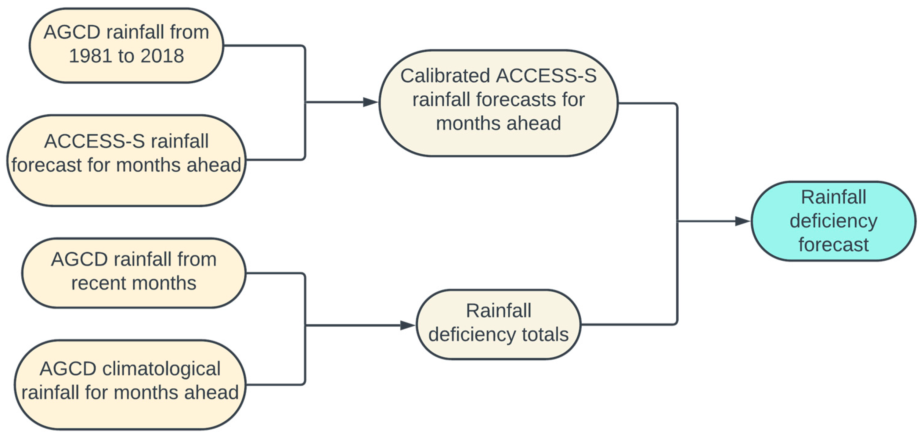
2.1. Inputs

The deficiency forecast product is created through the combination of three inputs. These inputs are summarized in

Table 1. Summary of datasets used to create the deficiency forecast product.

Dataset	Source and Description	Purpose	Example Start and End Dates for January 2022 3-Month Deficiency Forecast (Total of 4 and 6 Months after Forecast Is Included)
Existing deficiency grid	AGCD. The observed rainfall grid for a period was compared to grids from the corresponding historical period to determine the percentile of the observed rainfall. From this, a grid was created where cells were classified as being in deficiency if their percentile was below the 10th percentile.	Indicates which grid points are already in deficiency. This allows analysis of how existing deficiency areas will change. The end date of this grid is the end of the month before the starting month of the forecast. The start date is based on how long of a deficiency period is being considered.	Monthly and seasonal start date: October 2021 Monthly and seasonal end date: December 2021
Rainfall deficiency grid	AGCD. The observed rainfall for a period was subtracted from the climatological lowest decile for a period that covers both the observed period and the forecast period (referred to as the total period). This produced a grid where positive values indicate the amount of rainfall needed over the forecast period to ensure a deficiency is not present at the end of the total period. Negative values indicate that a grid cell is not at risk of being in deficiency (even if no rain is forecast, the area will not be in a deficiency at the end of the total period as the observed rainfall is more than enough to keep the total period out of deficiency)	Indicates how much rainfall is needed over a period to ensure a grid point is not in deficiency. The end date of this grid is the end of the month, which matches the ending month of the forecast. The start date is based on how long of a deficiency period is being considered.	Monthly and seasonal start date: October 2021 Monthly end date: January 2022 Seasonal end date: March 2022
Ensemble forecast of rainfall	A total of 99 calibrated ACCESS-S2 rainfall ensemble members were processed to form a single ‘super-ensemble’ file. Each ensemble member is a grid that indicates how much rainfall is forecast for the monthly or seasonal forecast period.	The forecast of each member is compared to the rainfall deficiency amount at each grid point. The proportion of forecasts that do not reach the threshold is used to define the forecast chance of being in a deficiency.	Monthly and seasonal start date: January 2022 Monthly end date: January 2022 Seasonal end date: March 2022

.

A deficiency refers to observed rainfall being in the lowest decile of the rainfall record for a particular period (this period is referred to as the ‘[observed] deficiency period’). The rainfall record began in 1900. The period used in the naming of the product does not include the forecast period. For example, 3-month deficiency monthly and seasonal forecasts have a total period of 4 months and 6 months, respectively, as the monthly and seasonal forecast periods extend the 3-month observed period by 1 month and 3 months, respectively.

AGCD is a gridded rainfall dataset formed using the Optimal Interpolation (OI) algorithm and in situ rain gauge data [18]. Rain gauge data are used to make adjustments to a background field created from interpolated station climatology to minimize the error variance of the resultant analysis. AGCD contains an error-checking routine where stations are excluded if an intermediate analysis formed from their exclusion is exceptionally different to one formed from their inclusion [19]. Its reliability severely decreases over gauge-sparse regions such as large parts of the interior of Australia [19], and it likely overestimates rainfall during the dry season over northern Australia [20]. The version of AGCD used in this study had a spatial resolution of 0.05° × 0.05° and is formed on a monthly timescale.

ACCESS-S rainfall forecasts are derived from the BOM Australian Community Climate and Earth-System Simulator-Seasonal version 2 (ACCESS-S2) model, a coupled dynamical ocean–atmosphere climate model that became operational in October 2021 ([21]. This study uses the operational forecasts, which contain 99 ensemble members produced using a time-lagged approach. The forecast for each period is an aggregate of daily forecasts. This study was limited to post-October 2021 because the ACCESS-S2 model was only operationalized then. The hindcast period of the model is from 1981 to 2018 but the ensemble size of these hindcasts is limited to 27 members. This makes the prediction of extremes less reliable and limits the usefulness of the hindcasts as a useful indication of the operational performance of this tool.

Calibrated ACCESS-S forecasts refer to ACCESS-S rainfall forecasts that have been corrected using a quantile-to-quantile correction to AGCD over a hindcast period. Distributions for the forecast and observational data from 1981 to 2018 are created, across an 11-day window centered on the forecast target date. The forecast values are then adjusted to the observational values that have the same ranking in the observational distribution as the forecast values had in the forecast distribution. This procedure cannot be applied to extremes in the forecast distribution, or the forecast values would be limited to the extremes of the observational record. Thus, for extreme values, a ratio of the observed and forecast value from the 2nd-lowest or 2nd-highest percentile is applied to the forecast value to adjust it. A cap is also applied so that the forecast value does not exceed the 1 in 100-year observed daily rainfall value. For additional detail on the calibration process, readers are referred to Griffiths et al. (2023) [22].

The utilization of forecasts calibrated to the same dataset used for determining the observed deficiencies and the deficiency thresholds is important to enable a direct comparison between the two datasets. Like AGCD, the accuracy of the calibrated forecast also degrades over gauge-sparse regions of Australia, with the lack of observations affecting both the amount of information available for the model to assimilate, as well as for calibration. It is not uncommon for the uncalibrated forecast to match or exceed the performance of the calibrated forecast over extremely gauge-sparse regions such as the northern interior of Western Australia. The resolution of the calibrated forecasts used was 0.05° × 0.05°, matching that of the observed rainfall dataset.

2.2. Creation of the Deficiency Forecast Grid and Plot

Python was used to process the rainfall deficiency and forecast grids into the probability of deficiency grids, as well as to visualize these probabilities as maps. The input data exist in NetCDF format, and, thus, Xarray was used for processing [23], with Matplotlib being used for visualization [24].

The deficiency forecast was computed for each grid point. If the rainfall deficiency amount was less than or equal to zero, the grid point was classified as not at risk of being at a deficiency. For grid points where the rainfall deficiency amount was positive, the forecast rainfall from each member of the ensemble (from a total of 99 members) was compared to the rainfall deficiency amount (which acted as a threshold). The proportion of members that did not exceed this threshold thus provided the chance of that grid point being in deficiency at the end of the total period (a period spanning the observed deficiency period and the forecast period). Mathematically, this can be expressed as Equation (1).

$$D{F}_i (\%)=\frac{{\sum }_{m=1}^{99}(F_{i,m}>D_i)}{99}\times 100$$

(1)

DF_i refers to a rainfall deficiency forecast, F_i,m refers to a forecast ensemble member, and D_i refers to a deficiency amount, while subscript i refers to a particular grid point and subscript m refers to a particular ensemble member. The inequality is taken to return a Boolean value (i.e., 1 if F_i,m is greater than D_i, 0 if F_i,m is not greater than D_i).

A schematic showing the workflow of how the final deficiency forecast is produced from the inputs is shown in Figure 1.

Both the monthly and seasonal forecasts are used while the deficiency period can be selected. Changing the deficiency period changes the length of the observed period analyzed; this is combined with the forecast period, which remains as one month or three months. Deficiency periods much longer than the forecast period (e.g., over 9 months) become less useful because forecast rainfall over one month or three months is less able to have an impact on deficiencies that have developed over a longer period. Without a loss of generality (as the skill of the deficiency forecast is largely determined by the skill of the rainfall forecasts, which are the same regardless of the deficiency period chosen), total periods of 4 months and 6 months were chosen for verification. These represent the monthly and seasonal forecast, respectively, combined with an observed deficiency period of 3 months, which is representative of the development of drought on a shorter timescale [25].

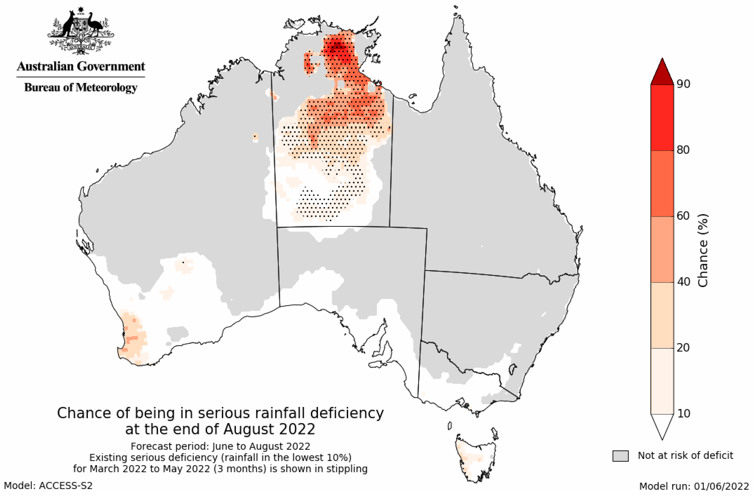
This grid could then be visualized spatially through a contour plot. The existing deficiency grid is overlain to facilitate analysis of the expected change in the extent of existing deficiency areas. An example of a deficiency forecast map is shown in Figure 2.

2.3. Verification Method for the Quantitative Metrics

The deficiency forecast grids were verified over 12 months from June 2022 to July 2023. The length of this verification period was limited by the availability of the forecast grids, which only allowed the deficiency forecast to be generated back to June 2022. The 12 months after this earliest date were chosen for verification to provide an analysis over a full year.

Three verification routines (Percent Correct, Brier Score, and Relative Operating Curve) were employed. These metrics were selected as they are common validation metrics for ensemble rainfall forecast verification [26] and are used operationally at the BOM.

The Percent Correct (PC) is a simple metric that calculates the hit rate of the forecast. A forecast ‘hit’ refers to when the outcome was predicted successfully by the majority of the ensemble members (i.e., no deficiency was observed for a forecast chance of less than 50% and a deficiency was observed for a forecast chance greater than or equal to 50%). The perfect PC value is 100%. Four different PC metrics were computed to evaluate the performance of the overall forecast, as well as six sub-sets. These scenarios (along with acronyms used hereafter for them) were as follows:

• Overall PC (PC-O). All grid points were evaluated.
• Deficiency PC (PC-D). Grid points where a deficiency eventuated were evaluated (how well were drought areas forecast).
• No-deficiency PC (PC-ND). Grid points where a deficiency did not eventuate were evaluated (how well were non-drought areas forecast).
• Existing deficiency PC (PC-ED). Grid points where there was an existing deficiency were evaluated (how well were changes to existing drought areas forecast).
• Non-zero forecast PC (PC-NZF). Grid points where the forecast probability was non-zero were evaluated (how well were areas forecast to have a chance of drought verified).
• Forecast deficiency PC (PC-FD). Grid points where the forecast probability was greater than 50% were evaluated (how well were areas forecast to be in drought verified).

The Brier Score (BS) is designed for evaluating probabilistic forecasts of a categorical outcome. It is equivalent to the mean squared difference between the forecast probabilities and the outcome (which is converted to a 1 or 0 for having occurred or not, respectively). The perfect BS value is 0. It is represented by Equation (2).

$$BS=\frac{1}{N}\sum _{i=1}^N{\left(f_i-o_i\right)}^2$$

(2)

N is the number of grid points, f is the forecast probability, and o is the outcome (0 if there was not a deficiency, 1 if there was), with subscript i referring to the values at a grid point.

The Area Under Curve (AUC) metric is related to the Relative Operating Characteristic curve (ROC curve) of the forecast. The ROC curve is a plot of the true positive rate of the forecast against its false positive rate at various forecast probabilities. The AUC is a statistic that quantifies the ROC curve and indicates how well the forecast has distinguished between deficiency and no-deficiency outcomes. A value of 1 is perfect, while a value of 0.5 indicates that the forecast has performed as well as a random classifier.

3. Results

3.1. Quantitative Metrics

The mean of the statistics across the study period is shown in

Table 2. Summary of the Percent Correct (PC) statistics from the monthly and seasonal forecasts.

	Monthly	Seasonal
PC-O	0.98	0.96
PC-D	0.44	0.21
PC-ND	0.99	0.97
PC-ED	0.80	0.79
PC-NZF	0.85	0.99
PC-FD	0.47	0.15
BS	0.0095	0.028
AUC	0.99	0.95

.

All the metrics except PC-D suggest that the forecast, on average, is skillful. The forecasts perform well when forecasting the eventual state of no deficiency, including for areas that have existing deficiencies.

The poorer results for PC-D suggest that the forecasts struggle with predicting the eventuation of deficiencies. The number of observed deficiency cells was lower than the number of forecast deficiency cells for 10 out of the 12 months, indicating that the poor performance was not due to underpredicting the occurrence of drought cells, but due to mismatches in the positioning of observed and forecast cells. For observed deficiency cells, the system was still able to provide some indication of the possibility of deficiencies eventuating, with the mean forecast probability being 36% for cells over the period. This is better than a system based on climatological probabilities, where the mean forecast probabilities for deficiencies eventuating would be 10%.

Furthermore, PC-FD was below 50%, indicating low skill when the forecast was predicting drought. The calculation of the signed difference indicated that in all 7 months where the forecast hit rate for this category was lower than 50%, low skill was due to the overprediction of drought probabilities. In the remaining months, there was also an overprediction of drought probabilities with only one month out of the five having a positive signed difference.

Given that the majority of grid points did not experience drought during this period, the other PC metrics did not reveal the seemingly poor skill of the forecasts in predicting eventual deficiency areas.

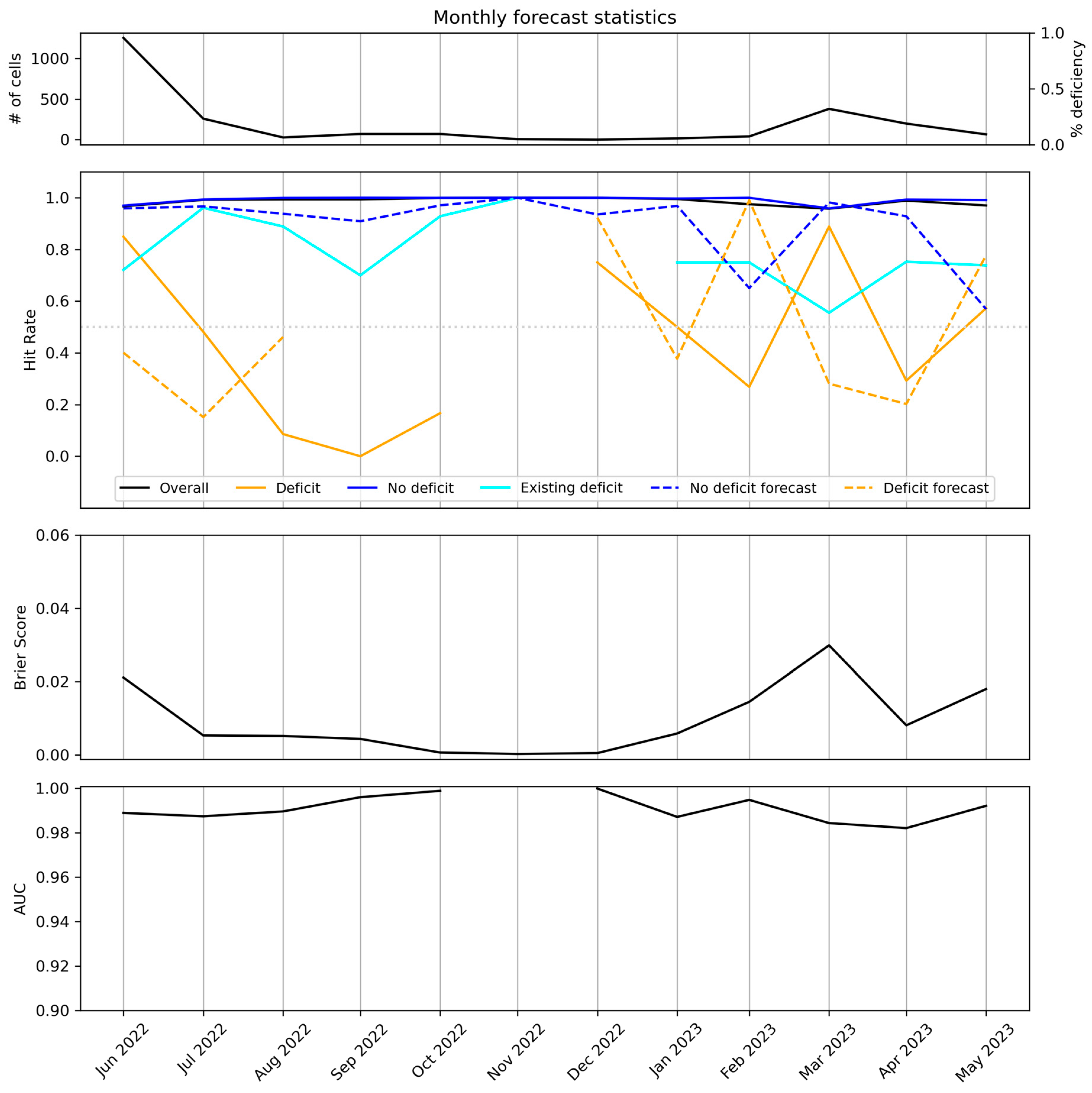
To analyze the presence of temporal trends, the time series of the metrics for the monthly forecast is presented in Figure 3.

The time series for PC-D and AUC was discontinuous in November 2022 because there were no deficiency grid cells for that month. Similarly, PC-FD was discontinuous from August 2022 to December 2022 as there were no forecast grid cells for those months.

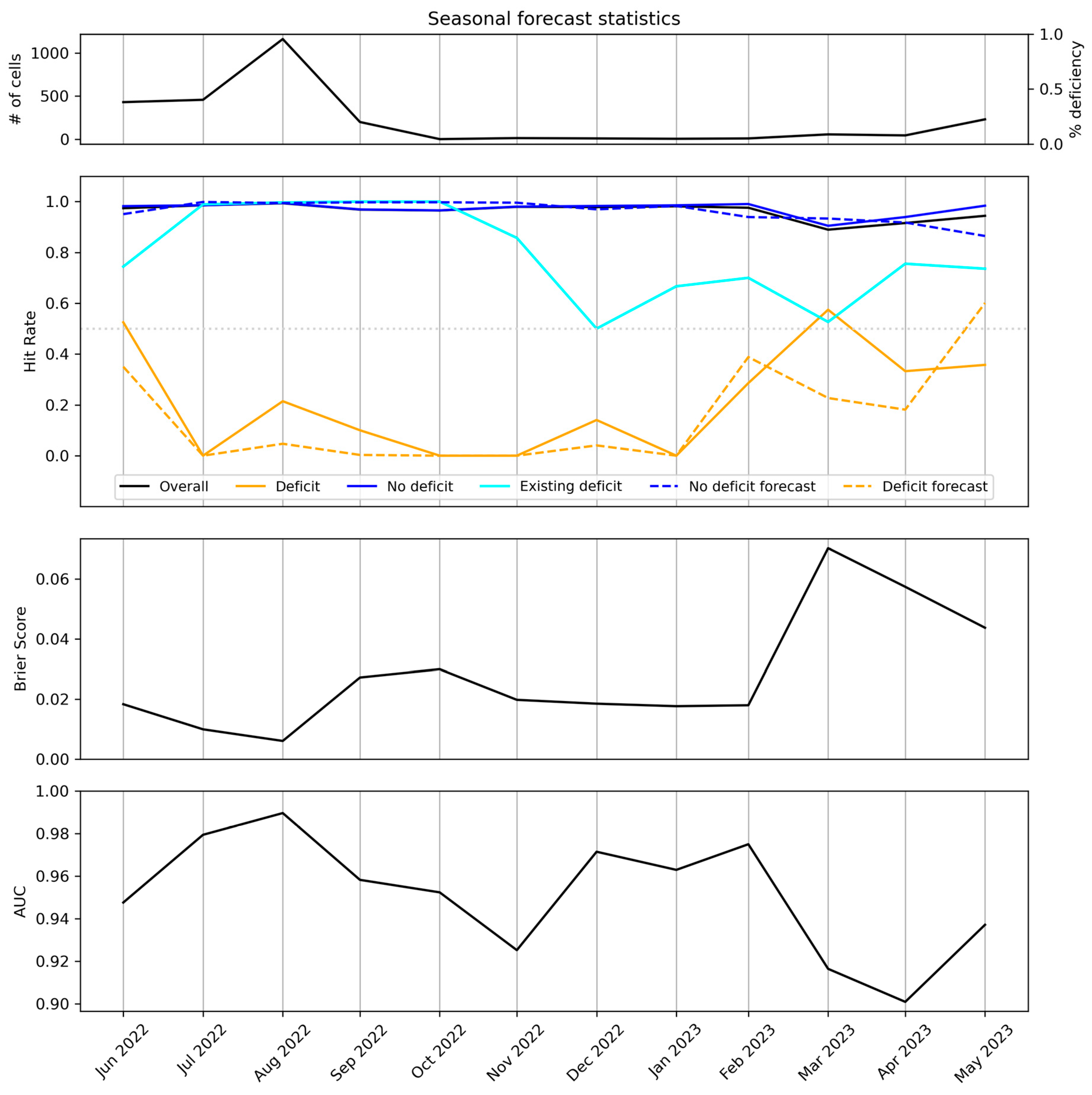
The PC-D hit rate was low from August 2022 to October 2022. The time series of metrics for the seasonal forecast is shown in Figure 4.

The PC-D and PC-FD hit rates were noticeably low from July 2022 to February 2023. The seasonal results are slightly worse than the monthly statistics, with this reduction in performance being particularly marked for the PC-D and PC-FD hit rates. A reduction in performance on the seasonal timescale would be natural given its inclusion of longer forecast lead times.

3.2. Visual Analysis

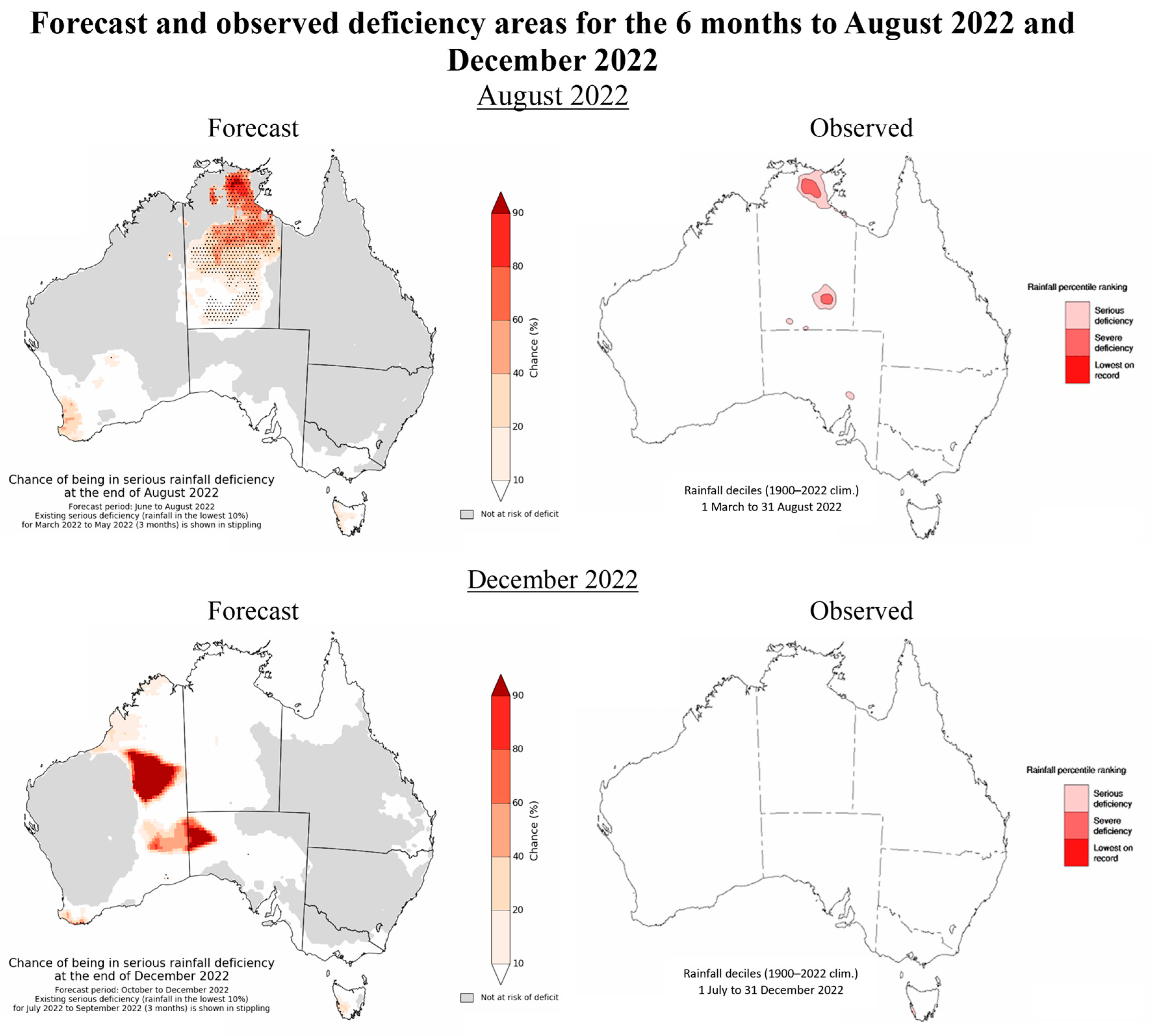
The forecast plots from two months are displayed to enable a visual analysis. A visual analysis facilitates the identification of spatial patterns and other aspects of performance that cannot be elucidated by quantitative metrics. It also helps readers to better understand the product and how it can be used. August 2022 was chosen because of its relatively good performance, while December 2022 was chosen as an example of a poorly performing month. The seasonal forecast plots are displayed alongside the observed deficiency that eventuated for those forecasts in Figure 5.

The value of the August 2022 forecast is evident from Figure 5. Over the Northern Territory (NT), much of the state was already in a deficiency on a 3-month timescale at the end of May. The forecast indicated that at the end of August, it was more likely than not that deficiency areas over southern and central NT would cease to exist. The observed deficiencies demonstrate this was largely the case. Additionally, the deficiency area that remained over the Top End of the NT corresponded with an area of high forecast probability (greater than 80%). There were some small areas of low forecast probabilities over south-west Western Australia and south-west Tasmania. These low probabilities are consistent with the fact that these areas did not end up observing deficiencies.

The December 2022 forecast highlights a key reason why the forecast performed poorly in terms of PC-FD. There are areas of very high forecast probabilities over the interior of Western Australia which are in stark contrast to the lower probabilities forecast over the remaining areas of northern and south-west Western Australia and south-west Tasmania. These unrealistic forecast areas are a result of the model struggling to represent threshold-based forecasts when the threshold is a very small number.

In this scenario, these areas are affected by the northern Australian dry season, which typically receives very little rainfall over the 6 months of July to December. As the amount of rainfall received over this period is very small, the threshold for being in deficiency is also very low. Many of the forecast ensemble members will forecast very low or zero rainfall, thus resulting in these areas technically falling into deficiency. These scenarios should be viewed with lower significance given the very small amounts of rainfall involved. This issue is compounded by the very low gauge density over some interior parts of the country (including areas with artifacts in the December 2022 forecast), which leads to a significant deterioration in the quality of both the observed and forecast rainfall over these areas. Note that over these areas, artifacts are evident when the risk of deficiency is non-zero; when it is zero, the deficiency forecast is not applicable and correspondingly masked on the maps (such as in the August 2022 forecast).

Other BOM long-range forecasts also show unrealistic artifacts over these areas during this time of the year. Inspection of other months revealed that this scenario was also resulting in the low performance of the PC-FD in months where the northern Australia dry season was relevant.

3.3. Comparison to the Unusually Dry Forecast

The closest BOM operational product to the forecast deficiency forecast detailed in this study is the ‘Chance of Unusually Dry rainfall forecast’. This forecast predicts the likelihood that rainfall over the forecast period will be in the lowest quintile of the hindcast period (from 1981 to 2018). Consequently, it is also known as a Quintile 1 (Q1) rainfall forecast.

Although both products provide an indication of where rainfall will be significantly below average, the two products are notably different in nature. The most obvious difference is that the threshold for dryness in the Q1 forecast is easier to satisfy, as it is based on the lowest quintile, compared to the lowest decile in the deficiency forecast. The Q1 rainfall forecast does not consider any past information and is, therefore, unable to contextualize where unusually low rainfall may be most significant.

There is also a fundamental difference in their algorithms. The Q1 forecast is based on determining the lowest quintile threshold for the forecast period (based on the historical hindcast record) and comparing this threshold against individual ensemble members to calculate the proportion of the ensemble that is below this threshold.

In the deficiency forecast, the threshold is based on actual observed data from a recent preceding period. It is not the lowest decile threshold of the forecast period that is relevant, but rather the threshold needed to be exceeded so that the rainfall total across both the observed and forecast period is not in the lowest decile. As such, it does not rely on a comparison to hindcast climatology like the Q1 forecast.

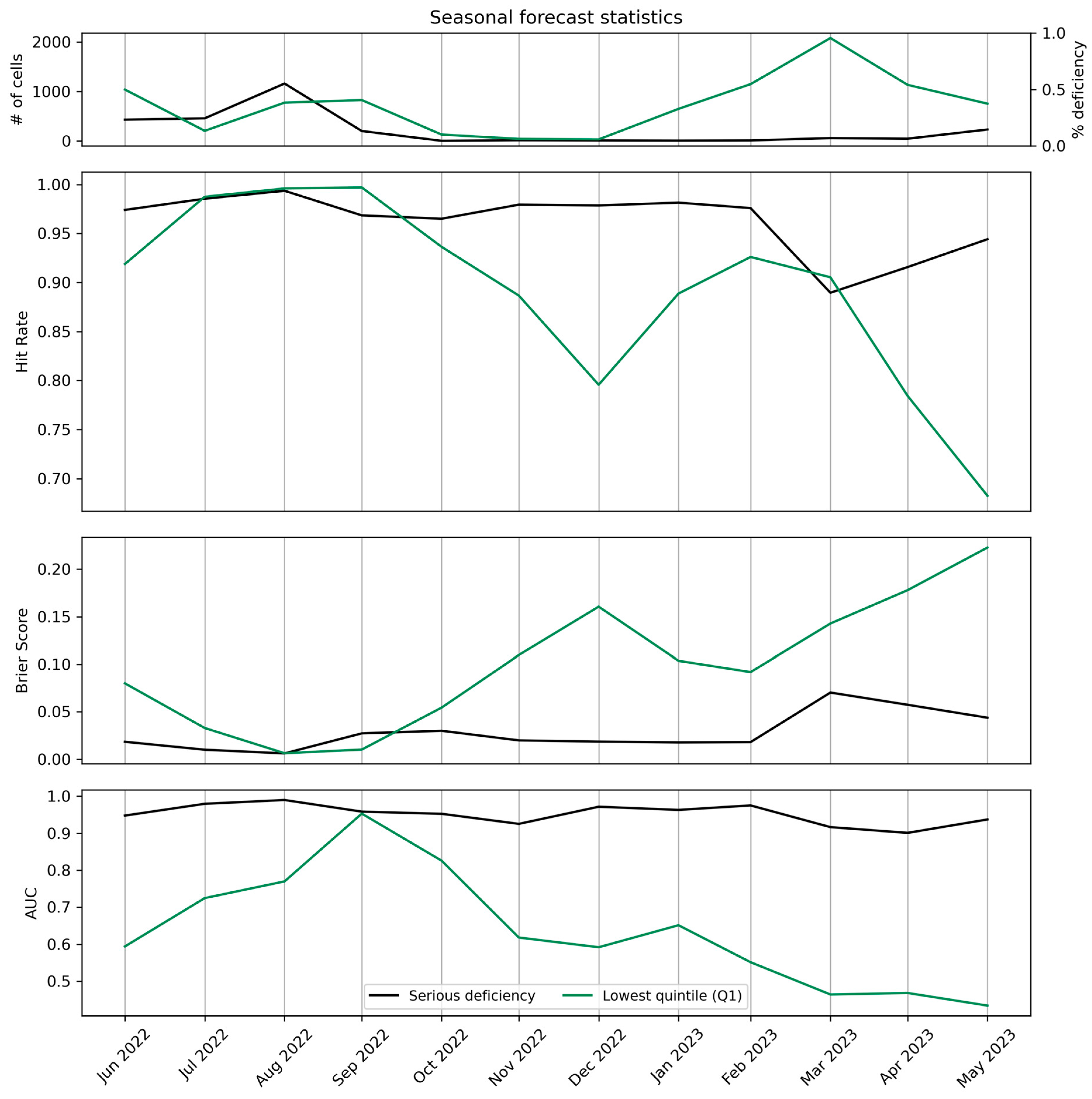
Quantitative metrics were recalculated for the Q1 forecast over the same period and using the same methodology used in Section 3.1. The observational quintile dataset provided by the BOM was created at a lower resolution of 0.25° × 0.25°. Consequently, the Q1 forecast was re-gridded to this resolution using bilinear interpolation. The number of observed deficiencies, overall PC BS, and AUC of the Q1 forecast compared to the deficiency forecast are shown in Figure 6.

For most of the period, the Q1 forecast had poorer performance than the deficiency forecast with the exception of September 2022. The performance of the Q1 forecast also seemed to be lower when there was a greater number of observed Q1 cells, an opposite trend to that observed for the deficiency forecast. The trend of observed Q1 was somewhat different to that of the observed serious deficiencies, with a peak in observed Q1 occurring in March 2023. This highlighted the difference that can exist due to the varying definitions of what is considered a deficiency (the lowest quintile for the forecast period in the Q1 forecast, the lowest decile over the total period for the deficiency forecast) as rainfall may be in Q1 but not in the lowest decile. Nonetheless, for both the Q1 forecast and the deficiency forecast, the proportion of deficiency cells was low across the study period (less than 1%), with very few cells observed from October to December 2022.

The Q1 forecast had poor performance for the prediction of observed deficiencies, worse than the deficiency forecast which demonstrated value. The mean forecast probability for cells that eventually observed deficiencies was 23% for the Q1 forecast, compared to 36% for the deficiency forecast. Note that a system based on climatology would be expected to have a mean forecast probability of 20% for the Q1 forecast, compared to 10% for predicting the lowest decile areas in the deficiency forecast. Over this study period, the Q1 forecast was only marginally better than climatology at predicting observed Q1, while the deficiency forecast was significantly better than climatology.

Special discussion will be given to the low hit rates for observed and forecast deficiencies, as these results stand out from the set of otherwise well-performing metrics.

3.4. Low Hit Rates for Observed and Forecast Drought

This result suggests that the product is not very good at predicting the development of deficiencies, but there are important subtleties to explore. As noted in Section 3.1, PC-FD is low due to a general overprediction of deficiencies. Combining these two findings suggests that the PC-FD and PC-D of the product are low not because the product is unable to represent the development of deficiencies, but rather because there is a mismatch in locations between the predicted deficiency cells and the observed deficiency cells. Calculation of the difference between the number of forecast and observed deficiency cells shows that for the period of low performance from July 2022 to February 2023, all months except February 2023 had more forecast deficiency cells than observed deficiency cells. These numerical statistics also do not consider the spatial performance of the forecast. It is possible that the forecast plots could provide valuable information on the trend of deficiency areas developing, even if the exact cells are not forecast correctly.

Furthermore, on average, the system still computed a non-trivial forecast probability (around 36%) for observed deficiencies. The PC-D only registered a hit if the probability of a forecast cell was greater than 50%. The low PC-D was not due to complete forecast misses but instead due to the forecast probabilities not being confident enough. The months with the poorest performance were also the months with the lowest proportion of deficiencies (October 2022 to February 2023), with the mean forecast probability for observed deficiencies improving to 42% when these months were excluded. The system performed better than climatology, where the mean forecast probability for deficiencies would be expected to be 10%.

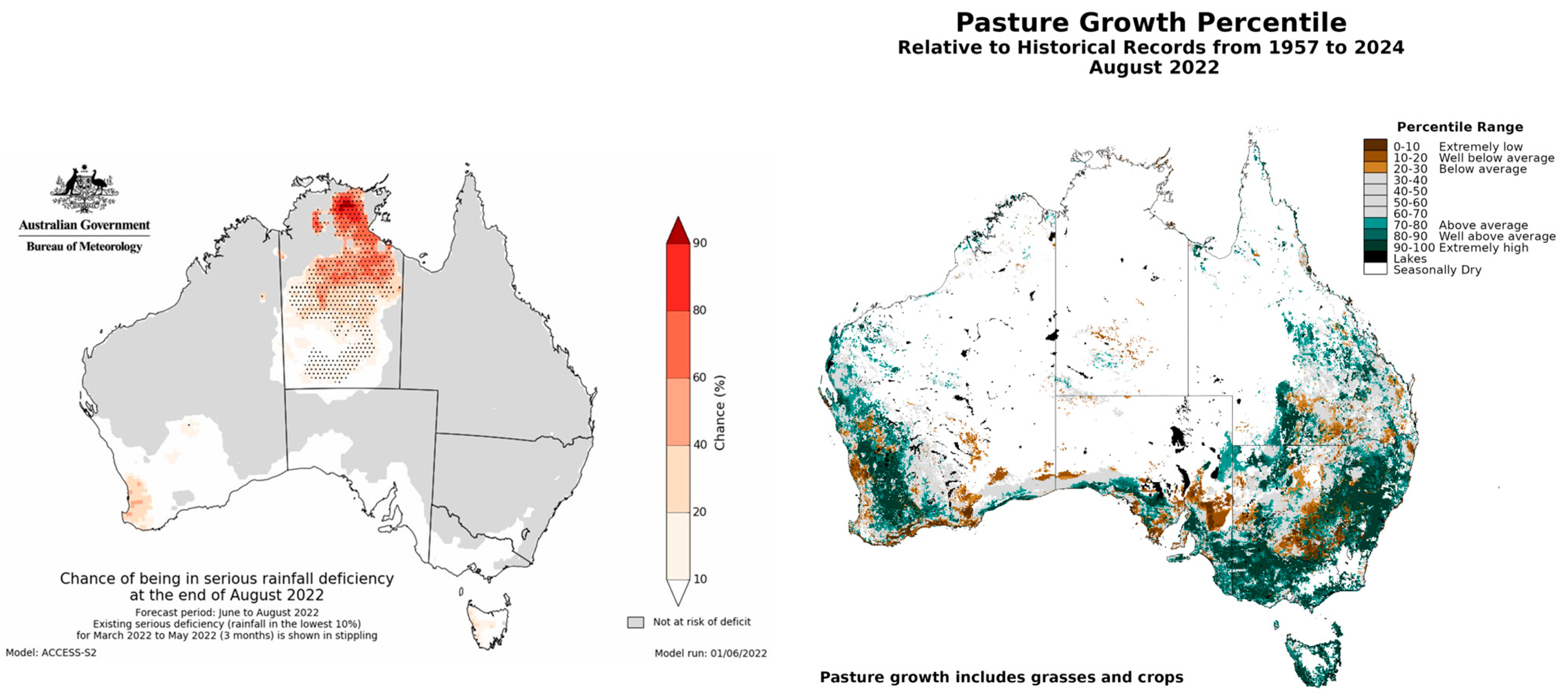
On a related note, even though areas with elevated deficiency forecast probabilities might not have ended up in serious deficiency, they may still have experienced dry conditions and drought impacts. To highlight a case of this, the August 2022 forecast is shown alongside a map from Aussie GRASS (Australian Grassland and Rangeland Assessment by Spatial Simulation) [27], a pasture growth model, in Figure 7.

Aussie GRASS simulates pasture growth by accounting for its biophysical processes, with the Aussie GRASS map revealing areas where pasture growth is below average. Pasture growth is moderately correlated to rainfall and a significant reduction in pasture growth can be an indication of drought [29]. It is evident from Figure 7 that there is a large overlap in deficiency forecast areas and reduced pasture growth, indicating the value the deficiency forecast can have in indicating areas of potential drought concern, which may not be identifiable through solely using observed rainfall data.

Importantly, an inspection of the visual plots in Section 3.2 revealed that the low PC-FD rates for some of the months were occurring over areas that had climatologically low rainfall over those periods. The small amounts of rainfall involved meant that the threshold for falling into deficiency was very small. The forecast amounts were also very small or zero, resulting in the forecast suggesting that there was a high chance of deficiencies occurring, even if the small amounts of rainfall involved meant these deficiencies were not particularly significant.

The accuracy of the forecast rainfall is a critical part of the system and is expanded upon in Section 4. Areas that have poorly performing rainfall forecasts would very likely perform poorly in the deficiency forecast too. A possible improvement could be to mask areas where the ensemble spread is large, as this indicates high model uncertainty and low confidence in the individual ensemble members. The rainfall forecast in these areas (and subsequently, the deficiency forecast) should be considered unreliable. A mask could also be considered for areas where the deficiency amount is very low and hence not meaningful; this is already employed in some BOM forecasts.

3.5. Does Performance Change When Drought Areas Are Increasing?

In this study, the forecast data were limited to existing data only from June 2022. Apart from resulting in only a short period of data for verification, the number of deficiency grid cells is very low in this period (less than 1% as seen in Figure 3 and Figure 4). This 12-month period followed three successive La Niña years, resulting in the small number of deficiency grid cells observed. The performance of the product was better when there was a larger number of deficiency cells (such as June 2022 and March 2023 for the monthly forecast, and August 2022 for the seasonal forecast), which is promising. Verifying the product for a period with a much larger number of deficiency cells would be of high value to properly assess this link, especially given that the product has an increased value when deficiencies are prevalent.

The presence of a correlation of performance with the trend of drought areas was also considered. Both PC-D and PC-FD had correlations greater than 0.7 with the number of deficiency grid cells, which suggests the performance of the product may be better when the number of deficiency grid cells is increasing. However, again, a longer study period with more variability would be required to more confidently assess this.

4. Discussion

This section will focus on placing the results of this study within the context of existing literature, as well as outlining possible future research directions.

As mentioned in Section 1, other drought forecast systems exist and have been validated, with the majority performing well (e.g., [10,11,14,30]). However, these systems provided forecasts that were deterministic and categorical or index-based, in contrast to the probabilistic forecasts produced by this system. This study is novel because of its direct use of rainfall totals (both observed and forecast) to determine the probability of an area being in meteorological drought. This allows an objective and physically consistent forecast to be made, which increases robustness and intelligibility.

Additionally, some of these studies [10,30] utilized a past drought event as a case study to demonstrate the value of their system. Such validations are effective at proving a system’s ability to forecast the occurrence of drought but performance during non-drought periods is often not well analyzed, if at all. The product produced in this study was probabilistic, allowing verification to be completed objectively across both non-drought and drought conditions. By being probabilistic, its utility for making risk management decisions is increased, compared to a deterministic forecast [15]. The data can also be visualized as probabilistic risk maps, allowing drought risk to be more easily communicated [15].

The use of the lowest decile as a characterization of drought has commonly been used and has historical pertinence [5], though this system could easily be modified to utilize a different percentile. Previous studies have found the use of deciles to be one of the most valuable indicators of meteorological drought (e.g., [3]), though an evaluation of the effectiveness of deciles as an indicator of drought is not the purpose of this study. The BOM drought-monitoring tool also monitors ‘severe rainfall deficiencies’, which are defined as observed rainfall being less than or equal to the lowest 5th percentile. It is important to be conscious of how the use of long-term historical rainfall deficiencies can mean the non-stationary effects of climate change on drought are not properly assessed.

This study highlights the importance of improving the quality of AGCD, as it is not only a direct input to the deficiency forecasts but also used in the calibration of ACCESS-S forecasts. The performance of AGCD over gauge-sparse areas is strongly limited by the reduction in the availability of in situ data that can be used in the analysis [19]. Consequently, it is expected that the performance and value of the deficiency forecast are also reduced over these areas. The inclusion of alternative data sources, such as satellite data, has been shown to be effective at enhancing performance in these areas [19].

Areas that have poorly performing rainfall forecasts would very likely perform poorly in the deficiency forecast too. The uncertainty of the real-time forecast skill should be communicated to users to promote intelligent usage of the product. A possible improvement could be to mask areas where the ensemble spread is large, as this indicates high model uncertainty and low confidence in the individual ensemble members. The rainfall forecast in these areas (and subsequently, the deficiency forecast) should be considered unreliable. A mask could also be considered for areas where the deficiency amount is very low and hence not meaningful; this is already employed in some BOM forecasts.

As noted in earlier literature [15], it is likely that this methodology, being based on dynamical modeling, would be limited in its ability to capture drought state changes caused primarily by stochastic and short-term weather variability (e.g., the absence or presence of extreme rainfall events). This is particularly relevant for Australia, where drought development and recovery are strongly related to heavy rainfall days associated with synoptic weather systems [31]. Forecasting this chaotic element of the weather is a fundamental limitation at longer lead times, and it would be prudent to ensure users are aware of this limitation.

Future research should consider the use of a longer study period, which would allow the product to be evaluated for a much greater variety of rainfall contexts, including deficiency-heavy periods. Promisingly, the results seemed to be better for periods where there was a greater proportion of deficiency areas. Further analysis on the variance of skill with region could also be completed. Additionally, consideration of the product over different study domains would also assist in determining its universality, though it is essential that the forecasts used in the system have been calibrated to the observed dataset.

5. Conclusions

Drought is a complex natural hazard for which a universal definition does not exist. Consequently, a ubiquitous monitoring or forecast system also does not exist. To monitor drought, many existing systems rely on using observed data, with rainfall being a common variable used. In Australia, the drought-monitoring system of the BOM relies on tracking areas where serious rainfall deficiencies (i.e., rainfall in the lowest 10% of the historical record) have been observed over a particular period. Systems such as this do not take into account the additional context provided by forecast rainfall.

To the best of our knowledge, there is no current drought monitoring or forecast system in Australia that objectively and directly couples observed and forecast rainfall amounts. The methodology outlined in this study is an attempt at addressing this gap and is formed from comparing the calibrated rainfall forecasts from ACCESS-S ensemble members to thresholds based on the amount of rainfall required to not be in a serious rainfall deficiency at the end of the period spanning the observed deficiency period and the forecast period. This yields a gridded probabilistic forecast of the chance of being in a serious rainfall deficiency.

Verification of the developed experimental product was completed through the use of PC, BS, and ROC statistics, as well as visual analysis. A study period from June 2022 to May 2023 was used, with forecasts on monthly and seasonal timescales being evaluated. The product appeared to perform well from an overall perspective, as indicated by high PC, BS, and Area Under the ROC (AUC) scores.

The PC for observed and forecast deficiency (PC-D and PC-FD, respectively) was low, but there were subtleties involved. The low PC-FD seemed to be due to a mismatch in the location rather than in the extent of deficiencies being forecast, with the number of forecast deficiencies cells generally being greater than the observed deficiency cells. Where deficiencies were eventually observed, the system computed a mean forecast probability of 36% for these cells. This suggests that the system would still have demonstrated value as the forecast probabilities for observed deficiencies were generally non-trivial, but just not confident enough to register as hits for the PC-D. The system performed better than the ‘Chance of Unusually Dry’ rainfall forecast currently in use at the BOM, as well as a climatological forecast.

The low PC for forecast deficiencies was at least in part due to difficulties in dealing with very low rainfall amounts associated with the northern Australia dry season, an issue afflicting other long-range forecasts from the BOM. The product appeared to generally perform well in forecasting the state of existing areas of deficiency, as well as eventual areas of no deficiency. However, the analysis was complicated by the low proportion of deficiencies in the study period (with less than 1% of the total domain being in deficiency across each of the months in the study period).

Given the overall positive results, the product could plausibly provide reasonable value, though it would be important to monitor its performance over a longer period to achieve a more thorough understanding and evaluation of its nature. The direct link between the observed and forecast data is novel and ensures a physically consistent system, as well as improving user comprehension.