Abstract
Climate change is increasingly influencing the water cycle, hindering the effective management of water resources in various sectors. Lazio, central Italy, exhibits a wide range of climatic conditions, stretching from the Tyrrhenian coast to the Apennines. This study assessed a crucial aspect of climate change, focusing specifically on reference evapotranspiration (ETo) and its associated hydrological variables. The seasonal Mann–Kendall (MK) test was used to assess trends in gridded data. The K-means algorithm was then applied to divide Lazio into four homogeneous regions (clusters), each characterized by distinct trends in hydrological variables. The analysis revealed statistically significant increasing trends (p ≤ 0.01) in temperature, solar radiation, and ETo, with more marked effects observed in the coastal and hilly clusters. In contrast, statistically significant decreasing trends (p ≤ 0.01) were observed for relative humidity, while no statistically significant trends (p > 0.01) were observed for precipitation. This study’s methodology, combining trend analysis and clustering, provides a comprehensive view of ETo dynamics in Lazio, aiding in pattern recognition and identifying regions with similar trends.
1. Introduction
Evapotranspiration (ET), the combination of water evaporation from the soil or water surface and uptake by plants, is a key physical process in climate and hydrological systems related to water and energy balance. Since actual ET is difficult to directly measure [1], it is typically estimated using reference evapotranspiration (ETo), which is calculated from the soil evaporation and crop transpiration of a standard surface based on hydrology and micrometeorology. The FAO-56 Penman–Monteith method is typically used for these calculations [2]. ETo is a key factor in agriculture and the environment, serving as a crucial measure of atmospheric water demand [3] and unraveling water availability and consumption patterns in different environments. As such, it is critical to study climate change [4], water resource development and use, crop water demand management, and drought monitoring.
Climate change impacts the hydrological cycle [5], primarily through altering precipitation and temperature patterns [6], with consequences on water resources and their use [7]. These effects vary considerably across regions due to specific climates and geographical features (e.g., altitude and proximity to the sea). One observable consequence is the weakening of the 500 hPa geopotential height gradient between the polar and mid-latitude regions in the Northern Hemisphere since 1979 [8]. As a consequence, areas like the UK are showing an increase in precipitation, driving higher runoff and evapotranspiration [9]. This southward shift of the North Atlantic jet stream in summer leads to increased cyclonic activity and wetter summers in northwest Europe, while the Mediterranean experiences fewer storms and dry summers [10,11]. This shift has significantly increased aridity in the Mediterranean region, especially after 1990 [12].
To effectively address potential imbalances in regional water management, a spatiotemporal analysis of ET trends is crucial. Established methods like the Mann–Kendall (MK) test [13,14] and Sen’s slope estimator [15] are employed to identify trends in hydrometeorological time series. Thus, due to the great diversity of climates worldwide, ETo trends can vary considerably depending on local climatic characteristics [16].
Extensive research has been carried out on ET trends in the Mediterranean (due to the increasing aridity in this region), which has revealed contrasting trends in ET across the region. Chaouche et al. [17] observed increasing ETo trends near the coast in Southern France using the MK test, while the annual precipitation (P) remained largely unchanged. Similarly, Gocic and Trajkovic [18] employed the MK test to analyze monthly FAO-56 Penman–Monteith equation [2] ETo data in the Balkan region. Their findings indicated the most significant upward trends in July and August, with April exhibiting the least change. Elferchichi et al. [19] adopted a different approach in Apulia (Italy). They combined the MK test with progressive trend analysis to assess seasonal and annual changes in ETo over the period of 1950–2003. A positive long-term trend (1961–2014) in ET was observed by Tomas-Burguera et al. [20] across most sites in mainland Spain and the Balearic Islands. However, examining shorter periods (20–30 years) yielded contrasting results, highlighting the temporal variability within the region. Bouregaa [21] investigated the ETo trends in Algeria, characterized by a Mediterranean climate along the northern coast and by arid and semi-arid climates in the inland areas. The author revealed significant ETo increases, particularly in June, July, and August. Eastern regions showed faster trends, with May and July exhibiting peak values. The highest annual ETo trends were in northeastern areas like Biskra. Factors like temperature, radiation, and wind speed influence these trends, highlighting implications for water resource management.
Studies in tropical regions have also revealed contrasting ETo trends. Pandey and Khare [22] found an overall increase in annual ETo in the Narmada River basin, a region with a humid tropical climate in India, using the MK and Spearman rho (SR) tests. However, they also found negative trends in mean annual precipitation for many stations. Conversely, Jerin et al. [23] used a modified MK test in Bangladesh and detected an overall decreasing trend in the annual ETo. Studies in both semi-arid and arid areas of China also report contrasting trends. They indicate both decreasing [24,25] and increasing [26] ETo trends. In particular, Gao et al. [27] analyzed the daily reference evapotranspiration in the arid and semi-arid areas of the West Liao River basin of China based on the MK test. The authors showed a decreasing degree for 46.7% of the investigated stations, which was larger than the increasing degree for the other 53.3% of stations. In addition, they found a significant overall increase in air temperature and significant decreases in wind speed, solar radiation, sunshine duration, and relative humidity. Solaimani and Bararkhanpour Ahmadi [28] investigated ETo variations across various climatic regions of Iran, encompassing the colder northern regions, warm and dry central areas, and warm and humid south. They employed the MK test and Sen’s slope methods and found a significant increase in ETo in all zones. Notably, the effects were most pronounced near coasts and water sources. Al-Hasani and Shahid [29] analyzed potential evapotranspiration trends in Iraq using ERA5-Land data from 1981 to 2021. They showed a significant increase over four decades, except in parts of the eastern alluvial plain. Moreover, southwest Iraq had the highest increase, driven mainly by rising air temperatures, especially in summer.
Several studies have employed clustering algorithms to identify regions with similar ETo patterns. Xing et al. [30] employed the rotated empirical orthogonal function (REOF) clustering method to pinpoint eight homogeneous ETo regions in China, while Masanta and Vemavarapu [31] detected 18 such regions in India using a fuzzy dynamic clustering approach. Interestingly, the latter revealed contrasting trends within India: a significant decrease in the annual ETo for nine clusters in the north and a significant increase for three clusters in the south. Furthermore, Chen et al. [32] used the K-means algorithm to group weather stations in the northeastern plain of China based on their mean climatic characteristics (i.e., temperature, relative humidity, and radiation). Di Nunno et al. [33] proposed a combined approach for the Veneto region (Italy). They employed clustering to identify trends in precipitation and homogeneous ETo areas and then used the seasonal MK test to analyze temporal trends in precipitation and ETo.
The aim of this study was to comprehensively analyze ETo and related meteorological variables in the Lazio region of Italy. To achieve this, we employed the seasonal MK test to identify trends in air temperature, relative humidity, wind speed, solar radiation, precipitation, and, crucially, ETo. Subsequently, based on the seasonal MK test results, we performed clustering to identify homogeneous areas within the study region.
The choice of the Lazio region for this study is justified by several factors. Firstly, its diverse landscape offers a rich variety of environmental conditions, making it an ideal location for comprehensive analysis. Secondly, Lazio exemplifies the Mediterranean climate, serving as a model region for other areas with similar climatic characteristics. Moreover, concerns regarding water scarcity in the region underline the importance of studying variables such as ETo.
This study introduced a novel approach to spatially characterize ETo. Unlike conventional methods that rely solely on the entire time series data, we used the output of a trend analysis method (the seasonal MK test) for clustering. Analyzing only the entire time series or using basic statistical values like the mean fails to capture crucial spatial variations in trends. This clustering approach based on the seasonal MK test results offers enhanced sensitivity to local climate variations. By identifying areas (clusters) with distinct trends in meteorological variables, this study allows for a more nuanced understanding of how climate change is affecting different areas within the study region.
2. Materials and Methods
2.1. Study Area and Dataset
Nestled in central Italy, the Lazio region experiences a typical Mediterranean climate, characterized by hot, dry summers and mild, wet winters. This climatic pattern, coupled with the region’s diverse topography and fertile soils, establishes an optimal environment for a variety of agricultural activities. The flat plains and alluvial soils support the cultivation of cereals, vegetables, and orchards, while olive grows and vineyards flourish, producing high-quality olive oil and wine. Livestock farming is also prominent and contributes to the region’s agricultural economy. The distinct seasons of the Mediterranean climate are crucial in shaping crop growth cycles and influencing water requirements.
Effective water resource management is essential in the Lazio region due to its direct impact on agriculture and overall sustainability. The seasonal variability in precipitation in the Mediterranean climate poses challenges to water availability and requires careful water management strategies. Farmers rely on efficient irrigation practices to optimize water use and ensure crop productivity. Balancing the water needs of diverse crops with the natural water availability in the region is critical for maintaining agricultural yields and sustaining the local economy.
As a consequence, a proper investigation of ETo and related hydrological variables for the Lazio region is crucial for optimizing water management, enhancing agricultural productivity, promoting sustainable practices, and bolstering climate resilience in the face of the region’s Mediterranean climate and historical transformations.
The present study relies on the MADIA (Meteorological Variables for Agriculture: Daily Time Series for the Italian Area) gridded dataset, as detailed by Parisse et al. [34]. This dataset provides time series data for key agro-meteorological variables derived from the Fifth Generation of the European Centre for Medium-Range Weather Forecasts (ECMWF) Reanalysis (ERA5). ERA5 offers hourly surface data at a spatial resolution of 0.25 degrees (https://www.drought.gov/data-maps-tools/ecmwf-reanalysis-v5-era5 (accessed on 1 March 2024)), making it a valuable resource for studying climate and weather patterns over extended periods (in this case, from 1981 to 2022). The dataset encompasses daily time series for minimum (Tmin), mean (Tmean), and maximum (Tmax) air temperatures, minimum (RHmin) and maximum (RHmax) air relative humidity, wind speed at a height of 10 m above the ground (WS10), shortwave solar radiation (Rs), precipitation (P), and ETo computed based on the FAO-56 Penman–Monteith equation [2].
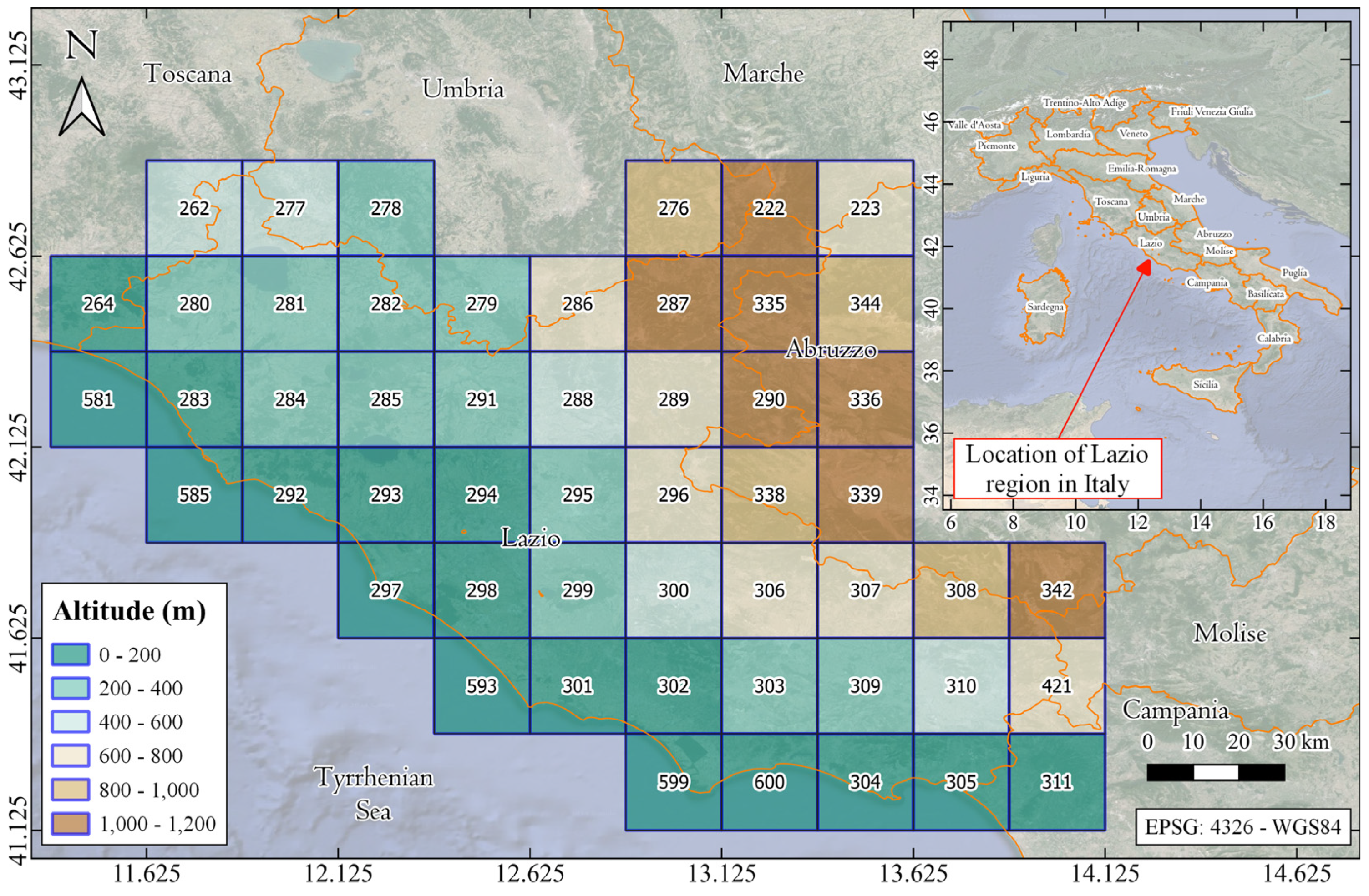
A total of 52 cells were considered, covering the entire continental territory of the Lazio region, including areas on the borders, which encompass neighboring regions such as Campania to the south, Abruzzo to the east, and Tuscany and Umbria to the north (Figure 1).

Figure 1.
Locations of the selected cells covering the Lazio region with an altitude representation.
2.2. Clustering
Clustering is a classification procedure that partitions an extensive dataset into a reduced number of groups. The objective of clustering is to unite akin data points by creating clusters in which the data within each cluster share resemblances, while the data in distinct clusters display some diversity [35].
In the current study, the K-means algorithm was employed to partition the Lazio region into homogeneous areas. The clustering procedure begins by treating each observation as a distinct cluster. It proceeds iteratively through two steps: identifying the pairs of closest clusters and merging them based on a specified linking criterion. This process continues until all clusters are merged. The distance between two clusters is assessed using the Manhattan distance formula:
where = {vi | i = 1, …, c} are the c centers of the clusters, is the data point belonging to the cluster, and is the distance between each data point and the cluster center , with the cluster center computed as:
where is the set of points related to the cluster. The Manhattan distance quantifies the separation between two points by adding up the absolute differences between each pair of variables [36]. In contrast, alternative distance metrics, such as the Euclidean distance, aggregate the squared differences in each variable. Consequently, if two data points are similar in most variables but differ significantly in one variable, the Euclidean distance could be disproportionately influenced by that single difference. Conversely, the Manhattan distance tends to be more robust, emphasizing the similarity of other variables and proving less susceptible to the impact of outliers [33].
It is important to note that the optimal number of clusters is not predetermined. Therefore, a preliminary analysis based on the silhouette technique was conducted to evaluate the appropriate clustering. Specifically, the silhouette score ranges from −1, indicating incorrect clustering, to 1, signifying well-defined and distinct clusters. Silhouette scores close to 0 suggest insignificant distances between clusters. The clustering procedure was performed using the Orange software (Version 3.32.0) [37].
2.3. Modeling Procedure
The modeling involved the combined utilization of the seasonal MK test and the K-means clustering algorithm (Figure 2), following the procedure outlined below:

Figure 2.
Flowchart of the modeling procedure.
- The seasonal MK test assessed the overall trends over the monthly time series in Tmin, Tmax, Tmean, RHmin, RHmax, WS10, Rs, P, and ETo. It is crucial to acknowledge that the time series data for the variables under investigation may exhibit various seasonal patterns. The seasonal MK test was implemented as an alternative to the conventional MK test, taking into account the seasonality in the estimation of the MK parameters. These parameters, primarily represented by Z, were used to identify statistically significant trends, with the confidence level set at 1% based on previous studies. The Z-statistic measures how many standard deviations a data point is from the mean, with its sign indicating the direction of the trend, being positive for an increasing trend and negative for a decreasing trend. Sen’s slope β was employed to assess the slope of the linear trend. Calculated by taking the median of all possible slopes between pairs of data points, positive and negative β-values signify increasing and decreasing trends, respectively. A comprehensive description of the seasonal MK test is provided in [33,38,39].
- The K-means clustering algorithm was then employed to identify homogeneous regions based on the seasonal MK parameters, Z and β, computed for each hydrological variable. The analysis of the results entailed a comparison of the distinct clusters determined by the silhouette score. The seasonal MK test parameters computed on each hydrological variable’s mean cluster time series were also discussed.
3. Results
3.1. Seasonal MK Analysis
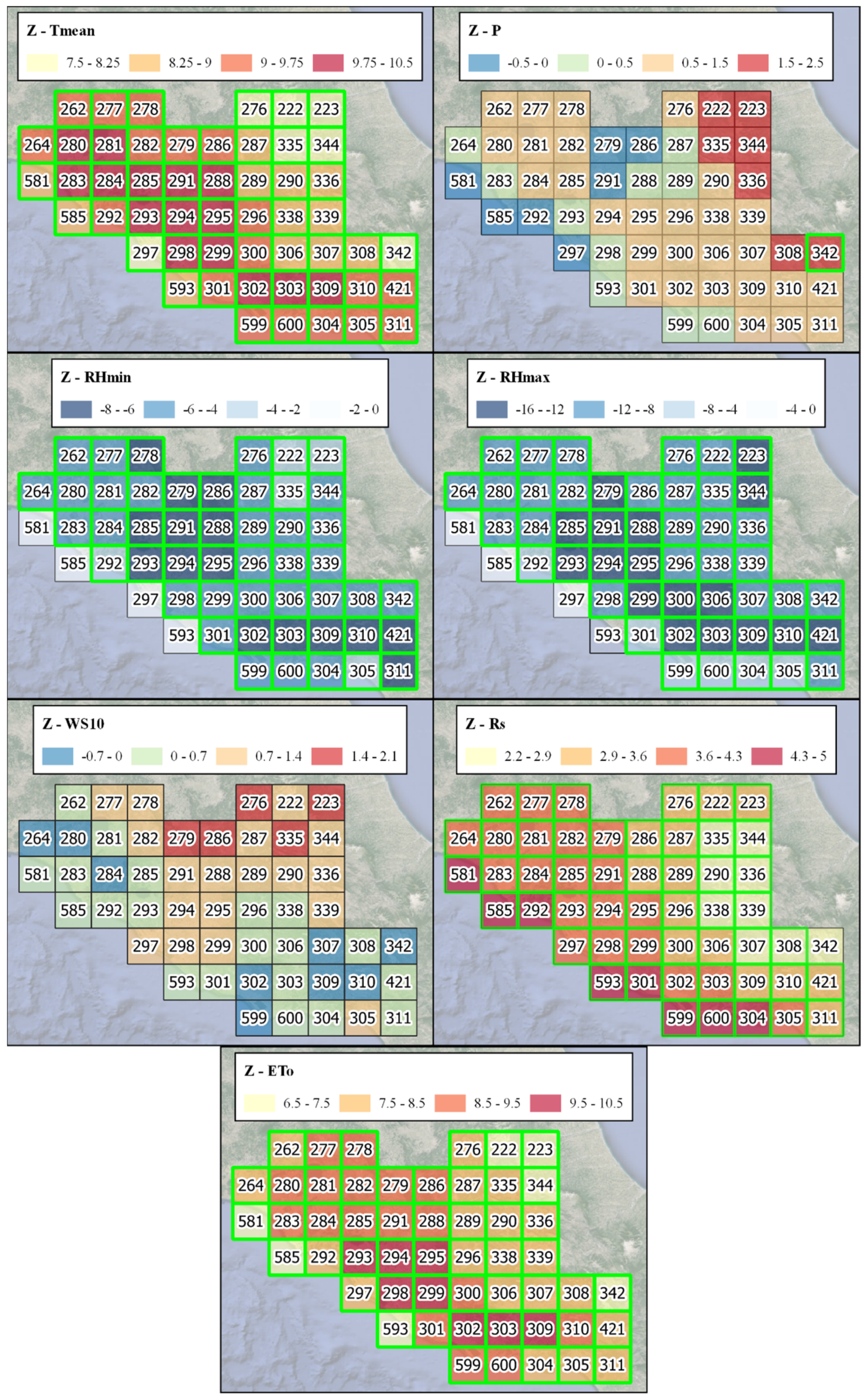
The monthly distributions of Z and β for the cells and hydrological variables are illustrated in Figure 3, with the p-values derived from the seasonal MK test marked on each plot (green cell border) as an indicator to assess clusters with notable trends. Previous studies on hydrological trends have conventionally set a significance threshold of p (at which trends are deemed significant) at 0.01 [40].
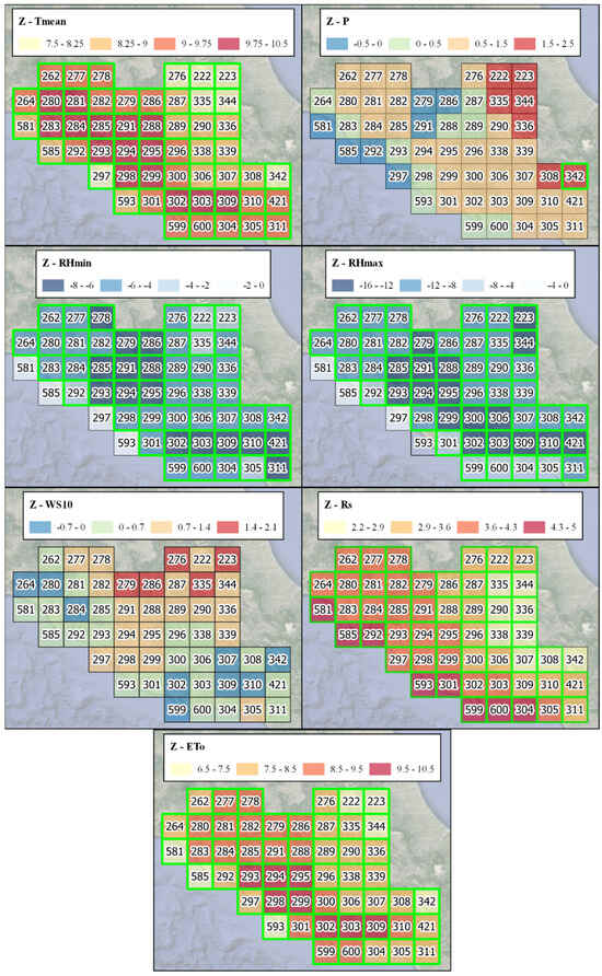
Figure 3.
Seasonal MK maps. Green-bordered cells indicate statistically significant trends.
For Tmean, statistically significant increasing trends were observed for all cells, with less marked trends in the inland mountainous areas (Z between 7.5 and 8.25) and more marked trends in the inland flat and hilly areas (Z between 9.75 and 10.5). Cells along the coast, especially in the central and northern areas, exhibited values closer to those in the inland mountainous areas. The observed lower temperature increases in the inland mountainous areas and higher increasing trends in the flat and hilly areas can be attributed to various geographical and environmental factors. Inland mountainous areas often have higher elevations, and as the altitude increases, temperatures tend to decrease due to the lapse rate. This phenomenon can lead to comparatively lower temperature increases in mountainous regions. Meanwhile, flat and hilly areas may experience higher temperature increases due to factors such as urbanization and heat absorption by surfaces like asphalt and concrete. At the same time, coastal areas are also influenced by ocean currents, which can impact local climate patterns and lead to lower Tmean increases compared with inland areas.
Regarding precipitation, trends were mostly positive, except for the northern coast and inland areas, where cells with slightly negative trends were observed. However, the trends were not statistically significant, except for one cell on the eastern border of Lazio, which showed a statistically significant increasing trend. A similar conclusion can be made for wind speed, which mostly exhibited positive trends, particularly in the northern inland area, with some areas on both the western and eastern borders showing slightly negative trends. However, no cells exhibited statistically significant trends. This suggests that while there may be localized fluctuations in precipitation and wind speed, they do not attain a degree of importance that would allow for conclusions regarding a uniform and widespread trend.
For relative humidity, statistically significant decreasing trends were observed for all cells, with the exception of a few cells along the central and northern coast. Slightly negative trends were observed in the inland mountainous areas (Z between −2 and 0), while more marked negative trends were observed in the inland flat and hilly areas (Z between −12 and 16 for RHmax). Inland mountainous areas, characterized by higher elevations, tend to experience less pronounced negative trends in RH due to their topography. As the altitude increases, the likelihood of moisture retention and reduced ET may contribute to slightly less marked decreases in RH compared with flat and hilly inland areas. Conversely, the inland flat and hilly areas, influenced by factors such as urbanization, exhibited more significant negative trends in RH. Urbanization, with surfaces like asphalt and concrete, can intensify heat absorption and decrease local humidity. Similar to the observed temperature trends, cells along the coast displayed RH values more closely resembling those in the inland mountainous areas. This might be influenced by coastal factors, such as ocean currents, which can modulate local climate patterns and contribute to the observed RH trends in these regions.
Solar radiation exhibited statistically significant increasing trends for all cells, with more pronounced trends observed in coastal areas (Z between 4.5 and 5). Slightly less marked trends were observed moving inland, with the least pronounced trends in the mountainous eastern area (Z between 2.2 and 2.9). One of the major factors contributing to the increase in solar radiation is climate change. Changes in atmospheric composition, such as increased greenhouse gases like carbon dioxide, can alter the Earth’s energy balance. This may result in more solar radiation reaching the Earth’s surface. Moreover, coastal areas often have a lower albedo than other surfaces. Albedo refers to the reflectivity of a surface. Water bodies have a lower albedo, meaning they absorb more sunlight than they reflect. As climate change and other factors lead to changes in surface properties, coastal areas may experience reduced reflectivity, contributing to increased solar radiation.
Finally, ETo exhibited statistically significant increasing trends for all cells, with less marked trends in the inland mountainous areas (Z between 6.5 and 7.5) and more marked trends in the inland areas close to the coast (Z between 9. 5 and 10.5). Overall, the seasonal MK test delved into the trends in ETo and established relationships with air temperature, precipitation, relative humidity, wind speed, and solar radiation. The comparison between the ETo and Tmean trends reveals that inland mountainous areas experienced less marked trends in both variables, which can be attributed to higher elevations and the lapse rate effect. Conversely, inland areas close to the coast displayed more pronounced trends in both ETo and Tmean, potentially influenced by coastal factors such as ocean currents and proximity to large water bodies. These findings align with the broader climatic context presented earlier. Coastal areas consistently resembled inland mountainous regions in both Tmean and RH trends, highlighting the intricate interplay of geographical and environmental factors.
In terms of RH, inland mountainous areas exhibited slightly negative trends, while flat and hilly areas showed more marked negative trends, which can be attributed to urbanization and, for some areas near the sea, water bodies. Therefore, the marked positive trends observed for ETo were accompanied by marked negative trends for RH. Indeed, an increase in ETo is often associated with warmer temperatures and higher ET rates, leading to a reduction in RH.
3.2. Clustering
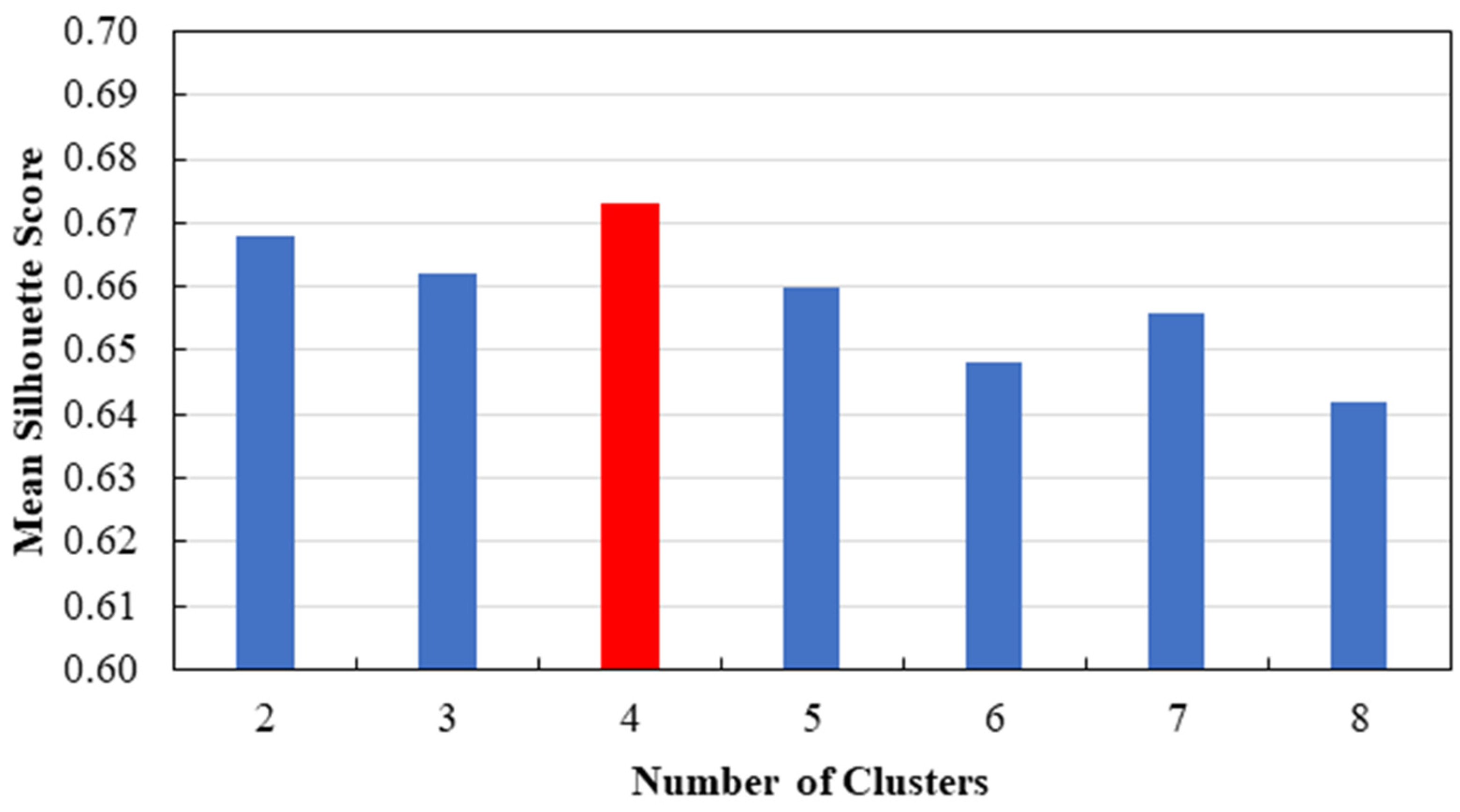
The optimization of the proper number of clusters was performed based on the silhouette technique. As shown in Figure 4, the best mean silhouette score, equal to 0.673, was obtained for a number of clusters equal to four, while the lowest mean silhouette score, equal to 0.642, was computed for eight clusters. It was, therefore, decided to divide the Lazio region into four clusters.

Figure 4.
Mean silhouette scores as a function of the number of clusters. In red the best mean silhouette score.
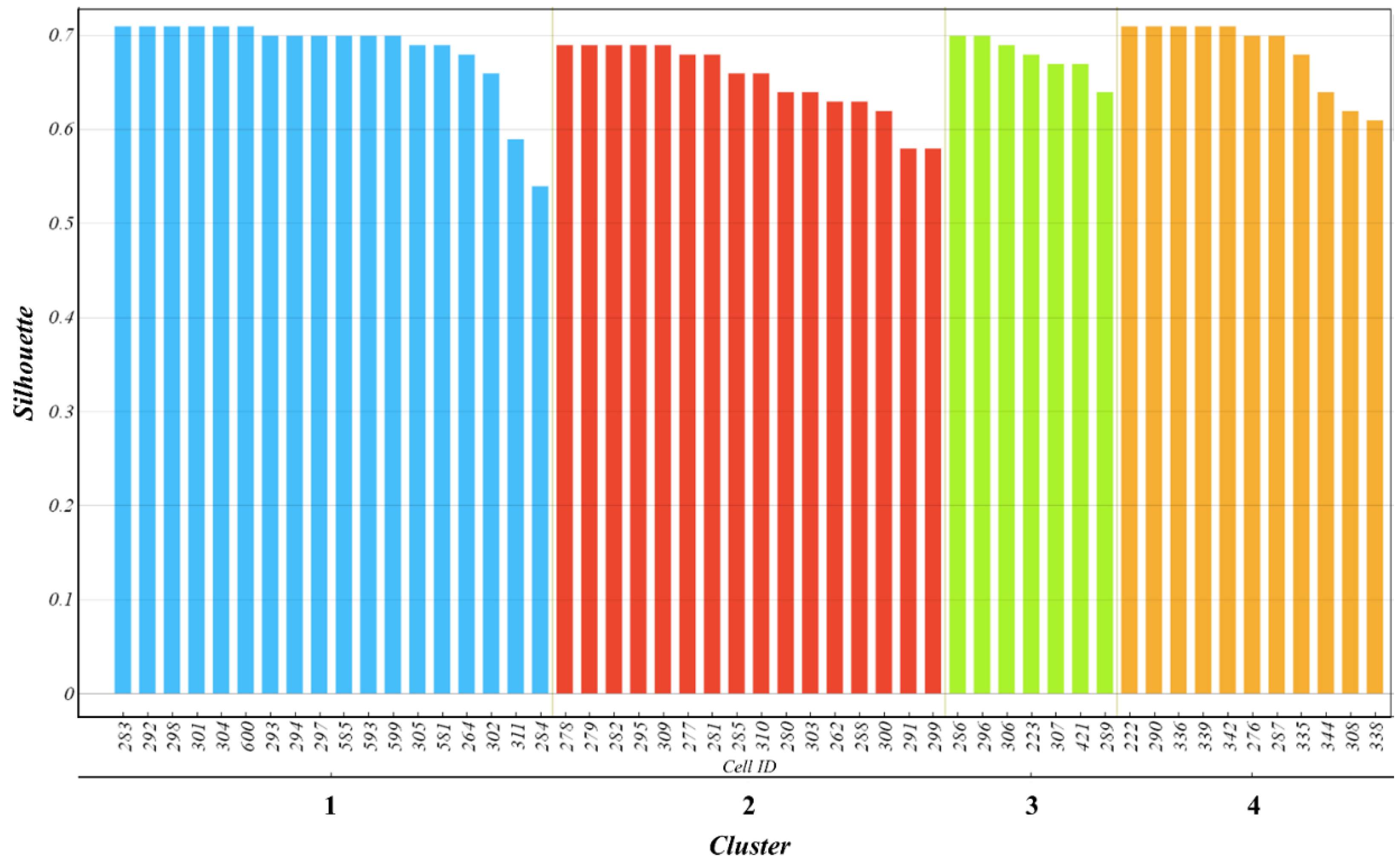
Figure 5 and Figure 6 illustrate the silhouette scores computed for all cells related to the four clusters and a representation of the clustering for the Lazio region, respectively. Moreover, Table 1 reports the mean values of the silhouette score, longitude, latitude, and altitude computed for each cluster. In contrast, Table 2 provides the mean, standard deviation, and coefficient of variation (CV) values computed in the mean cluster time series for each hydrological variable. Below is a description of the various clusters:
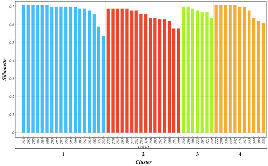
Figure 5.
Silhouette score values for each cell. Blue indicates cluster 1, red indicates cluster 2, green indicates cluster 3 and orange indicates cluster 4.
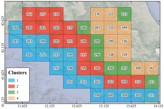
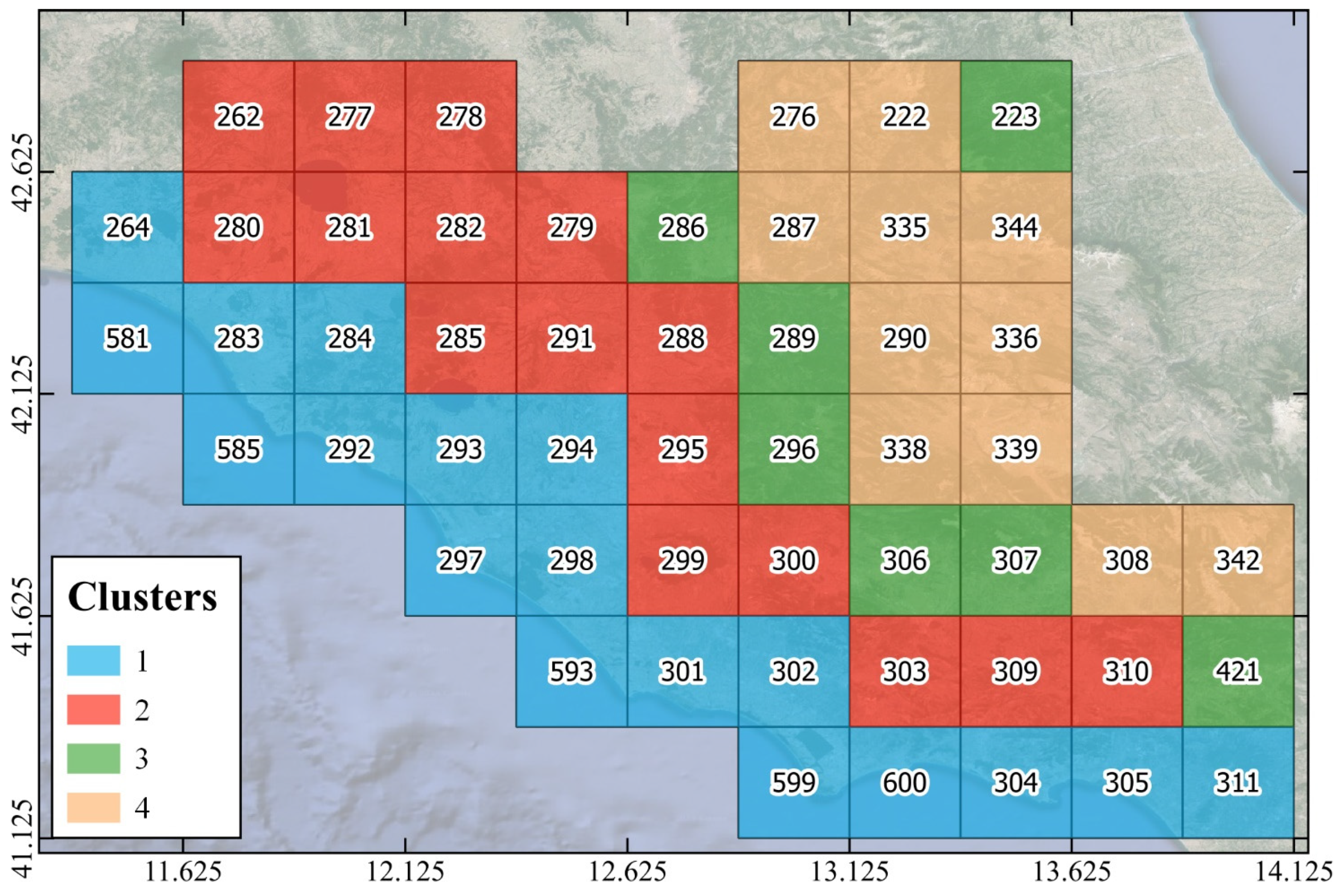
Figure 6.
Clustering of the Lazio region.

Table 1.
Mean values of silhouette score, longitude, latitude, and altitude computed for each cluster. The color bar ranges from white (low values) to green (high values).
Table 2.
Mean, standard deviation, and coefficient of variation (CV) values computed in the mean cluster time series for each hydrological variable. The color bar ranges from white (low values) to green (high values).
- –
- Cluster 1 corresponded to the coastal area of Lazio, with a mean altitude of about 102 m. The proximity to the sea resulted in the highest mean values of Tmean, RHmin, WS10, Rs, and ETo among the different clusters. At the same time, cluster 1 showed the lowest CV values for air temperature, relative humidity, and ETo. However, cluster 1 also exhibited the lowest mean values of P with the highest CV, indicating a high variability in precipitation. Overall, the proximity to the sea results in higher temperatures, increased solar radiation, and elevated ETo compared with inland areas. The higher heat capacity of the sea attenuates temperatures and prevents extreme fluctuations. The reflective surface of the Tyrrhenian Sea also plays a role, cooling coastal areas by reflecting solar radiation. Additionally, enhanced evaporation rates and the presence of sea breezes contribute to the region’s overall warmer and more stable climate, distinguishing it from the potentially more variable conditions experienced inland. In terms of silhouette scores, all cells showed values greater than 0.5, with the lowest value being 0.54 for cell 284. This can be explained by the proximity of this cell to cluster 2 to the north and east.
- –
- Cluster 2 covers the hilly area of Lazio between the coastal cluster 1 and the foothill cluster 3. Compared with cluster 1, cluster 2 exhibited lower means for Tmean, WS10, Rs, and ETo and higher means for RHmax and P. At the same time, it exhibited higher CV values for air temperature, RH, and ETo. The difference between clusters 2 and 1 in Lazio lies primarily in their altitudinal variations. Cluster 2, representing the hilly area, has a higher mean altitude of about 350 m, which leads to cooler temperatures and less solar radiation compared with coastal cluster 1. The topographical and altitudinal distinctions contribute to a cooler and potentially more variable climate in the hilly areas, highlighting the significant impact of altitude on regional climate patterns. Moreover, all cells showed silhouette scores greater than 0.5, with the lowest value of 0.58 for cell 299, explained by the proximity of this cell to cluster 1 to the south and west.
- –
- Cluster 3 covers the foothills of Lazio, with a mean altitude of about 690 m, between the hilly cluster 2 and the mountainous cluster 4. It also includes cell 223, which encompasses the foothills up to the border with Abruzzo and Marche. The location of cluster 3, far from the sea and close to the Apennines, led to a further reduction in the mean values of Tmean, WS10, Rs, and ETo and a further increase in the mean value of P, which was the highest among all the clusters. Cluster 3 also showed the lowest CV related to WS10 among all clusters. The combination of its location far from the sea and its proximity to the Apennines contributes to a more stable and uniform wind speed pattern. As for the silhouette scores, all cells exhibited values exceeding 0.64, indicating a robust affiliation with cluster 3.
- –
- Cluster 4 covers the Apennine area of Lazio, with a mean altitude of about 1037 m. Consequently, this area showed the lowest means for Tmean, WS10, Rs, and ETo among all clusters. At the same time, the CV values for Tmean and ETo were the highest among all clusters. Therefore, cluster 4 experiences more fluctuations or differences in both temperature and ETo, indicating a higher degree of variability in these specific climatic parameters within this cluster. However, cluster 4 also exhibited the highest mean value of RHmax. While the coastal areas also have high humidity, the specific mechanisms at play in mountainous terrain, such as orographic uplift and cooling, contribute to even higher relative humidity levels in these regions. As with cluster 3, all cells in cluster 4 showed a silhouette score higher than 0.6, confirming a robust affiliation with cluster 4.
The seasonal MK test was also performed for the mean cluster time series, computed for each hydrological variable. The outcomes of the test are reported in Table 3. Overall, all variables and clusters, with the exception of WS10 and P, showed statistically significant trends (p-values ≤ 0.01). In particular, Tmin, Tmax, and Tmean exhibited increasing trends, more marked along the coast and in the hilly areas (Z up to 9.84 for cluster 2), slightly less marked in the foothill and Apennine clusters, with the lower Z equal to 7.02 for cluster 4. Regarding RH, all clusters showed decreasing trends, with the hilly cluster 2 and the foothill cluster 3 showing the most marked negative trends, while less marked negative trends were observed for the coastal cluster 1. Regarding WS10 and P, although no statistically significant trends (p-values > 0.01) were observed, the overall trends were increasing for all clusters, more marked for the Apennine cluster 4 and less marked for the coastal cluster 1. When Rs and ETo were considered, increasing trends were observed for all the clusters. However, in this case, the most marked trends were observed for the coastal cluster 1 (Z up to 9.47 for ETo), while the less pronounced trends were observed for the Apennine cluster 4 (Z up to 7.98 for ETo).
Table 3.
Seasonal MK parameters computed in the mean cluster time series for each hydrological variable. The color bar ranges from yellow (low values) to red (high values) for the positive Z- and β-values, from blue (low values) to cyan (high values) for the negative Z- and β-values, and from green (≤0.01) to red (>0) for the p-values.
4. Discussion
The analysis carried out on the ETo in the Lazio region allowed the following to be highlighted:
- –
- The seasonal MK test was performed on each cell covering Lazio. The test exhibited statistically significant increasing trends in air temperature, solar radiation, and ETo while showing statistically significant decreasing trends for RH. Meanwhile, wind speed and precipitation showed both increasing and decreasing trends. However, in both cases, the trends were not statistically significant, indicating that the trends were not well-defined.
- –
- The clustering analysis based on the seasonal MK parameters led to a division of Lazio into four distinct clusters: the coastal cluster 1, the hilly cluster 2, the foothill cluster 3, and the Apennine cluster 4. Overall, a decrease in the mean values of Tmean, RHmin, WS10, Rs, and ETo was observed from the coastal area to the inland area. Nevertheless, with a decrease in temperature and solar radiation, there was a corresponding increase in the CV values of both Tmean and ETo with altitude. Indeed, the Apennine cluster 4 exhibited more pronounced fluctuations or variances in both temperature and ETo, indicating a higher degree of variability in these particular climatic variables with increasing altitude.
- –
- Finally, the seasonal MK test performed on the mean cluster time series showed statistically significant increasing trends for all clusters with respect to air temperature, solar radiation, and ETo, which were more marked for the coastal and hilly clusters 1 and 2. At the same time, statistically significant decreasing trends were observed for RH for all clusters, particularly in the hilly cluster 2.
Overall, the results obtained in the present study were consistent with long-term trend outcomes at both large and small spatial scales. Aschale et al. [41] investigated ET and soil moisture for flash droughts across Sicily. They observed a significant increasing trend for most months in the region using the MK test and Sen’s slope estimator. Similarly, results at a smaller scale for the Belice area in southwestern Sicily showed that variations in runoff and ET correlated with changes in precipitation and temperature, including an increase in potential ET [42]. Additionally, in the eastern Mediterranean, Tabari [43] identified a positive trend in ETo using the MK test and Sen’s slope estimator, with 70% of the meteorological stations in the western region of Iran showing this trend in the 1966–2005 time series. However, discrepancies were observed by Di Nunno et al. [33], who pointed out the absence of statistically decreasing trends in precipitation and ETo for the coastal clusters of Veneto. Furthermore, Chaouche et al. [17] reported both the absence of significant precipitation trends and increasing ETo trends for the Mediterranean coastal area of France. However, these results contradict those of Aschale et al. [44], who reported downward precipitation trends and no significant ETo trends for the Sicilian region. In addition, Di Nunno and Granata [45] explored ETo trends in Sicily, considering historical data and two climate scenarios based on different Representative Concentration Pathways (RCP 4.5 and RCP 8.5), employing a combined clustering–forecasting approach to detect three distinct clusters, all displaying increasing trends in ETo. Nonetheless, the discrepancies between the different studies can be attributed to numerous factors. On the one hand, these variations may be linked to the time series length and the meteorological stations’ spatial density. On the other hand, they may be influenced by the distinct characteristics of each study area, encompassing morphologies and microclimates. Such variations can lead to divergent findings even in regions with seemingly similar features.
This paper introduces a novel approach to climatic clustering for the Lazio region, setting it apart from conventional methods commonly found in the literature. Rather than relying on statistical parameters calculated from individual historical series, the clustering is based on the Z- and β-parameters of the seasonal Mann–Kendall test. This approach offers a novel perspective, leveraging the intrinsic seasonal patterns and trends captured by the seasonal MK test parameters. By doing so, this paper provides a different way to identify homogeneous regions based on climatic variables. This new approach not only advances climatic clustering methods but also helps us better understand regional climate variations and their impacts.
The importance of analyzing ETo trends in the Lazio region should be noted. The increasing ETo trends in Lazio significantly impact agriculture. Elevated ETo implies a higher water demand for crop evapotranspiration, potentially leading to water stress and reduced crop yields. This increased demand for water resources may exacerbate existing challenges in water availability and irrigation management. As a result, farmers may need to adopt more efficient irrigation techniques, invest in water-saving technologies, or adapt cropping patterns to mitigate the impact of elevated ETo. Furthermore, heightened ETo can contribute to soil moisture depletion, affecting soil fertility and structure. This, in turn, may necessitate adjustments in agricultural practices, such as improved soil conservation practices and increased use of organic matter to enhance water retention capabilities. Overall, understanding and adapting to the consequences of increased ETo is crucial for sustaining agricultural productivity in the Lazio region. This will require a comprehensive approach combining water management strategies, technological advancements, and customized agronomic practices to address the evolving climatic conditions.
It should be emphasized that while Lazio features diverse local climates, ranging from coastal to mountainous areas, a limitation of this study is that it did not take into account varying climates, such as arid or semi-arid areas. These areas often present distinct hydrological and climatic patterns, leading to more pronounced seasonal and annual fluctuations in variables such as evapotranspiration, precipitation, and temperature. Including these areas could lead to a more complete understanding of water cycle dynamics and climate change impacts. Additionally, arid and semi-arid areas frequently face water scarcity and management challenges, offering valuable insights into effective water resource management strategies that might be overlooked.
Future research could employ the current methodology to explore trends in crop ET, considering the specific crops grown in different areas of Lazio, each with distinct water requirements. This approach would yield additional insights into clustering and trends associated with both reference and crop ET. Alternative clustering algorithms and trend analysis methods could also be explored in subsequent research to bolster the credibility of the methodology. From this perspective, a high-resolution dataset of ET (e.g., [46]) as well as meteorological variables derived from ERA5-land could be used to check if the spatial resolution affects the clustering and trend analysis.
5. Conclusions
This study provided valuable insights into the spatiotemporal trends of ETo and related hydrological variables in the Lazio region. The seasonal MK test conducted on individual cells covering Lazio revealed statistically significant upward trends in air temperature, solar radiation, and ETo. Conversely, there were statistically significant downward trends observed in relative humidity. In contrast, wind speed and precipitation displayed both increasing and decreasing trends, but in both instances, these trends did not reach statistical significance, suggesting that the trends were not clearly defined. A key finding is the identification of four distinct clusters across the region, each with different patterns of ETo and the associated variables. These clusters spanned from the coastal region (cluster 1), progressed through the hilly (cluster 2) and foothill (cluster 3) areas, and culminated in the Apennine region (cluster 4). Overall, higher mean values of air temperature, solar radiation, and ETo were observed along the coastal and hilly areas, together with more marked increasing trends. At the same time, although the foothill and Apennine areas showed less marked trends, they exhibited marked fluctuations in both temperature and ETo, particularly marked for the Apennine cluster 4. The devised approach, which merges trend analysis and clustering methods, strives to offer a succinct and dependable assessment of the trends in ETo and associated hydrological variables. Additionally, it aims to pinpoint distinct regions with homogeneous trends. As a result, this approach stands as a valuable decision-making tool for water resource management, taking into consideration the spatiotemporal changes in hydrological variables across a water district.
Author Contributions
Conceptualization, F.D.N. and F.G.; methodology, F.D.N. and F.G.; software, F.D.N. and F.G.; validation, N.D., G.B., C.T. and G.d.M.; formal analysis, F.D.N. and F.G.; data curation, F.D.N. and F.G.; investigation, F.D.N., G.d.M. and F.G., writing—original draft preparation, F.D.N., N.D., G.B. and F.G.; writing—review and editing, F.D.N., N.D., G.B. and F.G.; visualization, F.D.N., N.D., G.B., C.T., G.d.M. and F.G.; supervision, F.G. All authors have read and agreed to the published version of the manuscript.
Funding
This research received no external funding.
Data Availability Statement
The MADIA gridded dataset was utilized in the development of this manuscript. The data are available at the following website: https://zenodo.org/records/7252361 (accessed on 30 April 2024).
Conflicts of Interest
The authors declare no conflicts of interest.
References
- Wanniarachchi, S.; Sarukkalige, R. A Review on Evapotranspiration Estimation in Agricultural Water Management: Past, Present, and Future. Hydrology 2022, 9, 123. [Google Scholar] [CrossRef]
- Allen, R.G.; Pereira, L.S.; Raes, D.; Smith, M. Crop Evapotranspiration: Guidelines for Computing Crop Water Requirements; Food and Agriculture Organization of the United Nations: Rome, Italy, 1998. [Google Scholar]
- Singer, M.B.; Asfaw, D.T.; Rosolem, R.; Cuthbert, M.O.; Miralles, D.G.; MacLeod, D.; Quichimbo, E.A.; Michaelides, K. Hourly potential evapotranspiration at 0.1° resolution for the global land surface from 1981-present. Sci. Data 2021, 8, 224. [Google Scholar] [CrossRef]
- Giménez, P.O.; García-Galiano, S.G. Assessing Regional Climate Models (RCMs) Ensemble-Driven Reference Evapotranspiration over Spain. Water 2018, 10, 1181. [Google Scholar] [CrossRef]
- Kundzewicz, Z.W. Climate change impacts on the hydrological cycle. Ecohydrol. Hydrobiol. 2008, 8, 195–203. [Google Scholar] [CrossRef]
- Lee, T.-H.; Lo, M.-H.; Chiang, C.-L.; Kuo, Y.-N. The maritime continent’s rainforests modulate the local interannual evapotranspiration variability. Commun. Earth Environ. 2023, 4, 482. [Google Scholar] [CrossRef]
- Wang, X.; Liu, L. The impacts of climate change on the hydrological cycle and water resource management. Water 2023, 15, 2342. [Google Scholar] [CrossRef]
- Christidis, N.; Stott, P.A. Changes in the geopotential height at 500 hpa under the influence of external climatic forcings. Geophys. Res. Lett. 2015, 42, 10798–10806. [Google Scholar] [CrossRef]
- Blyth, E.M.; Martínez-de la Torre, A.; Robinson, E.L. Trends in evapotranspiration and its drivers in Great Britain: 1961 to 2015. Prog. Phys. Geog. 2019, 43, 666–693. [Google Scholar] [CrossRef]
- Robson, J.; Sutton, R.T.; Archibald, A.; Cooper, F.; Christensen, M.; Gray, L.J.; Holliday, N.P.; Macintosh, C.; McMillan, M.; Moat, B.; et al. Recent multivariate changes in the north Atlantic climate system, with a focus on 2005–2016. Int. J. Climatol. 2018, 38, 5050–5076. [Google Scholar] [CrossRef]
- Dong, B.; Sutton, R.T. Recent trends in summer atmospheric circulation in the north Atlantic/European region: Is there a role for anthropogenic aerosols? J. Clim. 2021, 34, 6777–6795. [Google Scholar] [CrossRef]
- Bakke, S.J.; Ionita, M.; Tallaksen, L.M. Recent European drying and its link to prevailing large-scale atmospheric patterns. Sci. Rep. 2023, 13, 21921. [Google Scholar] [CrossRef] [PubMed]
- Mann, H.B. Nonparametric tests against trend. Econometrica 1945, 13, 245–259. [Google Scholar] [CrossRef]
- Kendall, M.G. Rank Correlation Methods; Griffin: London, UK, 1948; p. 202. [Google Scholar]
- Sen, Z. Innovative trend analysis methodology. J. Hydrol. Eng. 2012, 17, 1042–1046. [Google Scholar] [CrossRef]
- Granata, F.; Di Nunno, F. Forecasting evapotranspiration in different climates using ensembles of recurrent neural networks. Agric. Water Manag. 2021, 255, 107040. [Google Scholar] [CrossRef]
- Chaouche, K.; Neppel, L.; Dieulin, C.; Pujol, N.; Ladouche, B.; Martin, E.; Salas, D.; Caballero, Y. Analyses of precipitation, temperature and evapotranspiration in a French Mediterranean region in the context of climate change. C. R. Geosci. 2010, 342, 234–243. [Google Scholar] [CrossRef]
- Gocic, M.; Trajkovic, S. Analysis of trends in reference evapotranspiration data in a humid climate. Hydrolog. Sci. J. 2014, 59, 165–180. [Google Scholar] [CrossRef]
- Elferchichi, A.; Giorgio, G.A.; Lamaddalena, N.; Ragosta, M.; Telesca, V. Variability of Temperature and Its Impact on Reference Evapotranspiration: The Test Case of the Apulia Region (Southern Italy). Sustainability 2017, 9, 2337. [Google Scholar] [CrossRef]
- Tomas-Burguera, M.; Santiago Beguería Sergio, M. Vicente-Serrano Climatology and trends of reference evapotranspiration in Spain. Int. J. Clim. 2021, 41, E1860–E1874. [Google Scholar] [CrossRef]
- Bouregaa, T. Spatiotemporal trends of reference evapotranspiration in Algeria. Theor. Appl. Clim. 2024, 155, 581–598. [Google Scholar] [CrossRef]
- Pandey, B.K.; Khare, D. Identification of trend in long term precipitation and reference evapotranspiration over Narmada River basin (India). Glob. Planet. Chang. 2018, 161, 172–182. [Google Scholar] [CrossRef]
- Jerin, J.N.; Islam, H.M.T.; Islam, A.R.M.T.; Shahid, S.; Hu, Z.; Badhan, M.A.; Chu, R.; Elbeltagi, A. Spatiotemporal trends in reference evapotranspiration and its driving factors in Bangladesh. Theor. Appl. Climatol. 2021, 144, 793–808. [Google Scholar] [CrossRef]
- Xu, S.; Yu, Z.; Yang, C.; Ji, X.; Zhang, K. Trends in evapotranspiration and their responses to climate change and vegetation greening over the upper reaches of the Yellow River Basin. Agric. For. Meteorol. 2018, 263, 118–129. [Google Scholar] [CrossRef]
- Li, Y.; Yao, N.; Chau, H.W. Influences of removing linear and nonlinear trends from climatic variables on temporal variations of annual reference crop evapotranspiration in Xinjiang, China. Sci. Total Environ. 2017, 592, 680–692. [Google Scholar] [CrossRef] [PubMed]
- Fu, J.; Gong, Y.; Zheng, W.; Zou, J.; Zhang, M.; Zhang, Z.; Qin, J.; Liu, J.; Quan, B. Spatial-temporal variations of terrestrial evapotranspiration across China from 2000 to 2019. Sci. Total Environ. 2022, 825, 153951. [Google Scholar] [CrossRef] [PubMed]
- Gao, Z.; He, H.; Dong, K.; Li, X. Trends in reference evapotranspiration and their causative factors in the West Liao River basin, China. Agric. For. Meteorol. 2017, 232, 106–117. [Google Scholar] [CrossRef]
- Solaimani, S.; Bararkhanpour Ahmadi, S. Evaluation of TerraClimate gridded data in investigating the changes of reference evapotranspiration in different climates of Iran. J. Hydrol. Reg. Stud. 2024, 52, 101678. [Google Scholar] [CrossRef]
- Al-Hasani, A.A.J.; Shahid, S. Spatial distribution of the trends in potential evapotranspiration and its influencing climatic factors in Iraq. Theor. Appl. Climatol. 2022, 150, 677–696. [Google Scholar] [CrossRef]
- Xing, W.; Wang, W.; Shao, Q.; Yu, Z.; Yang, T.; Fu, J. Periodic fluctuation of reference evapotranspiration during the past five decades: Does evaporation paradox really exist in China. Sci. Rep. 2016, 6, 39503. [Google Scholar] [CrossRef] [PubMed]
- Masanta, S.K.; Vemavarapu, S.V. Regionalization of evapotranspiration using fuzzy dynamic clustering approach. Part 1: Formation of regions in India. Int. J. Climatol. 2020, 40, 3514–3530. [Google Scholar] [CrossRef]
- Chen, Z.; Zhu, Z.; Jiang, H.; Sun, S. Estimating daily reference evapotranspiration based on limited meteorological data using deep learning and classical machine learning methods. J. Hydrol. 2020, 591, 125286. [Google Scholar] [CrossRef]
- Di Nunno, F.; De Matteo, M.; Izzo, G.; Granata, F. Spatio-temporal analysis of reference evapotranspiration in Veneto: A combined clustering and trends analysis approach. Sustainability 2023, 15, 11091. [Google Scholar] [CrossRef]
- Parisse, B.; Alilla, R.; Pepe, A.G.; De Natale, F. MADIA-Meteorological variables for Agriculture: A Dataset for the Italian Area. Data Brief 2023, 46, 108843. [Google Scholar] [CrossRef]
- Di Nunno, F.; Granata, F. Spatio-temporal analysis of drought in Southern Italy: A combined clustering-forecasting approach based on SPEI index and Artificial Intelligence algorithms. Stoch. Environ. Res. Risk Assess. 2023, 37, 2349–2375. [Google Scholar] [CrossRef]
- Callahan, C.; Bridge, H. Data Mining of Rare Alleles to Assess Biogeographic Ancestry. In Proceedings of the Systems and Information Engineering Design Symposium (SIEDS), Charlottesville, VA, USA, 29–30 April 2021; pp. 1–6. [Google Scholar] [CrossRef]
- Demsar, J.; Curk, T.; Erjavec, A.; Gorup, C.; Hocevar, T.; Milutinovic, M.; Mozina, M.; Polajnar, M.; Toplak, M.; Staric, A.; et al. Orange: Data Mining Toolbox in Python. J. Mach. Learn. Res. 2013, 14, 2349–2353. Available online: http://jmlr.org/papers/v14/demsar13a.html (accessed on 1 March 2024).
- Hirsch, R.M.; Slack, J.R. A Nonparametric Trend Test for Seasonal Data with Serial Dependence. Water Resour. Res. 1984, 20, 727–732. [Google Scholar] [CrossRef]
- Di Nunno, F.; de Marinis, G.; Granata, F. Analysis of SPI index trend variations in the United Kingdom -A cluster-based and bayesian ensemble algorithms approach. J. Hydrol. Reg. Stud. 2024, 52, 101717. [Google Scholar] [CrossRef]
- Shahfahad; Talukdar, S.; Ghose, B.; Islam, A.R.M.T.; Hasanuzzaman, M.; Ahmed, I.A.; Praveen, B.; Asif; Paarcha, A.; Rahman, A.; et al. Predicting long term regional drought pattern in Northeast India using advanced statistical technique and wavelet-machine learning approach. Model. Earth Syst. Environ. 2024, 10, 1005–1026. [Google Scholar] [CrossRef]
- Aschale, T.M.; Peres, D.J.; Palazzolo, N.; Sciuto, G.; Cancelliere, A. Run analysis of potential evapotranspiration and soil moisture for investigating flash droughts in Sicily. In Proceedings of the EGU23, the 25th EGU General Assembly, Vienna, Austria, 23–28 April 2023. EGU-13360. [Google Scholar] [CrossRef]
- Liuzzo, L.; Noto, L.V.; Arnone, E.; Caracciolo, D.; La Loggia, G. Modifications in Water Resources Availability Under Climate Changes: A Case Study in a Sicilian Basin. Water Resour. Manag. 2015, 29, 1117–1135. [Google Scholar] [CrossRef]
- Tabari, H.; Marofi, S.; Aeini, A.; Talaee, P.H.; Mohammadi, K. Trend analysis of reference evapotranspiration in the western half of Iran. Agric. For. Meteorol. 2011, 151, 128–136. [Google Scholar] [CrossRef]
- Aschale, T.M.; Peres, D.J.; Gullotta, A.; Sciuto, G.; Cancelliere, A. Trend Analysis and Identification of the Meteorological Factors Influencing Reference Evapotranspiration. Water 2023, 15, 470. [Google Scholar] [CrossRef]
- Di Nunno, F.; Granata, F. Future trends of reference evapotranspiration in Sicily based on CORDEX data and Machine Learning algorithms. Agric. Water Manag. 2023, 280, 108232. [Google Scholar] [CrossRef]
- Singer, M.; Asfaw, D.; Rosolem, R.; Cuthbert, M.O.; Miralles, D.G.; Miguitama, E.Q.; MacLeod, D.; Michaelides, K. Hourly Potential Evapotranspiration (hPET) at 0.1degs Grid Resolution for the Global Land Surface from 1981-Present; University of Bristol: Bristol, UK, 2020. [Google Scholar] [CrossRef]

Disclaimer/Publisher’s Note: The statements, opinions and data contained in all publications are solely those of the individual author(s) and contributor(s) and not of MDPI and/or the editor(s). MDPI and/or the editor(s) disclaim responsibility for any injury to people or property resulting from any ideas, methods, instructions or products referred to in the content. |
© 2024 by the authors. Licensee MDPI, Basel, Switzerland. This article is an open access article distributed under the terms and conditions of the Creative Commons Attribution (CC BY) license (https://creativecommons.org/licenses/by/4.0/).