Global Warming Impacts on Southeast Australian Coastally Trapped Southerly Wind Changes

Abstract

Coastally trapped southerly wind changes are prominent during southeast Australia’s warm season (spring and summer). These abrupt, often gale force, wind changes are known locally as Southerly Busters (SBs) when their wind speeds reach 15 m/s. They move northwards along the coast, often producing very large temperature drops. SBs exceeding 21 m/s are severe SBs (SSBs). SBs have both positive and negative impacts. They bring relief from oppressively hot days but can cause destructive wind damage, worsen existing bushfires, and endanger aviation and marine activities. This study assesses the impacts of global warming (GW) and associated climate change on SBs and SSBs, using observational data from 1970 to 2022. Statistical analyses determine significant trends in annual frequency counts of SBs and SSBs, particularly during the accelerated GW period from the early–mid-1990s. It was found that the annual combined count of SBs and SSBs had increased, with SSBs dominating from 1970 to 1995, but SB frequencies exceeded SSBs from 1996 to 2023. The ascendency of SB frequencies over SSBs since 1996 is explained by the impact of GW on changes in global and local circulation patterns. Case studies exemplify how these circulation changes have increased annual frequencies of SBs, SSBs, and their combined total.

1. Introduction

Southerly wind changes, particularly in the form of southerly busters (SBs), which are defined as wind gusts of at least 15 m/s and strong southerly busters (SSBs) defined as gusts of at least 21 m/s [1], impact the southeast coast of Australia in the warm season (October to March). An SB passage is notable for the typical wind shift from northwesterly to southerly, and for the abrupt temperature decreases of up to 20 °C within minutes [2]. The SB is a gravity (or density) current, trapped against the coast by the Great Dividing Range (GDR), e.g., [3,4,5,6,7]. SBs typically are several hundred kilometers wide and up to about 1 km in depth above the ocean surface. The SB impacts can range from damage to coastal infrastructure and worsening of existing bushfires to aviation- and marine-related threats to life and safety. SBs frequently produce a pronounced drop in temperature, cooling uncomfortably hot days after its passage. SBs can produce low cloud, fog, and strong wind gusts. Consequently, SBs can pose a threat to human health and property, and can disrupt aviation and marine activities, changing the intensity and direction of bushfires. Aviation hazards of SBs include low-level wind shears and associated turbulence created by SBs. The major consequences occur during landing or take-off, when they can create sudden increases or reductions in airspeed and aircraft drift. The strong SB winds and accompanying low-level turbulence are also hazards for boats and rock fishers. Marine rescue organizations respond annually to thousands of emergency assistance requests [8], many related to the large waves and rough seas produced by SBs.

SBs have several alternative names. These include ducted coastal ridging, which is an atmospheric surge over coastal southeast Australia, moving at a speed of about 15–20 m/s at the leading edge of the ridge [9]. The coastal ridging is ducted along the coast and is then stabilized by inertial modification, decaying on a synoptic time scale of a few days along the NSW coast [9]. Another widely used term is coastally trapped disturbances (CTDs), following the study by Gill [10] of the coastal lows observed moving anticlockwise around southern Africa. Coastal lows are similar in structure to coastally trapped waves in the ocean. As in the case of SBs, temperature inversion conditions typical of the area prevent the escape of energy upwards, and the Coriolis effect traps energy against the high escarpment that borders the southern African coast. Hence, CTDs are produced because low-level flow in the synoptic-scale systems cannot cross the escarpment [10]. The term CTD has also been used frequently for southeastern Australian SBs [11,12,13,14]. Notably, the consensus is that the SB is a gravity current, also known as a density current, trapped against the coast by the GDR, e.g., [3,4,5,6,7]. As such, it is initiated by a synoptic scale system and is generated by the density difference between the cooler southerly flow and the in situ warmer environment ahead of the surge.

It has been suggested recently in the media that SBs and SSBs have become far less frequent and weaker in recent decades [15]. Aside from its importance as a phenomenon and the long association with relief from oppressively hot days, it is of interest to assess the impacts on SBs of long-term environmental changes in temperature and pressure. Of importance are those changes due to global warming (GW) that might have affected SB and SSB frequencies and intensities. Synoptically, the typical sequence, irrespective of the ENSO phase, is for high pressure over the Tasman Sea to direct warm to hot N/NW winds over the southeast Australian coast ahead of a Southern Ocean frontal system moving from west to east. The frontal system introduces a much cooler, denser air mass which travels much faster through Bass Strait due to less friction than further north over land. On archived, manually analyzed, mean sea level pressure (MSLP) synoptic charts, this appears as a ridge of high pressure extending from a high-pressure center in the Great Australian Bight (GAB) or further west. Once the colder, denser air behind the frontal system reaches eastern Bass Strait it turns northward, and the ridging continues parallel to the coast as a density current trapped by the higher topography parallel to the coast and to the west of the coastal plain.

An SB typically appears as a pressure surge northward along the southeast Australian coast, in the form of coastal ridging, as shown by the MSLP charts in Figure 1. Figure 1a shows the MSLP prior to the SB passage along the southern east coast and Figure 1b is after the SB passage.

Figure 2 is an image from the high temporal and spatial resolution of the Himawari-8 satellite at 0600 UTC, 7 October 2021. It shows clearly the abrupt wind change from NW to south along the coast near Sydney, associated with a recent SB passage. The southerly wind structure appears as a shallow, narrow coastal band of wind, which is shaped by high topography parallel to the coast further inland, where northwest to westerly winds prevail.

It is important to investigate future trends in the frequency and intensity of SBs to assess the possible impact of GW on SBs. Recent model impact studies point to an increase of over 35 °C per day [16,17], which might suggest a possible increase in SB intensity and/or frequency on Australia’s southeast coast, because the larger the density difference between air masses, the greater the potential for strong wind changes with SB characteristics. As far as the authors are aware, there are no recent observationally based studies investigating future trends in SBs related to global warming.

The first aim of this study is to produce a climatology of SBs and SSBs (using maximum gust thresholds defined above), from which changes in temperature and pressure characteristics can be related to SB strength frequency and strength, given that temperature and pressure are related to density through the equation of state. Second, trends in frequency and intensity of SBs are investigated using frequency plots, and permutation testing of interval means to investigate the relationships with increased global warming. The Introduction provides background information on the structure and physical processes involved with SBs. The Materials and Methods Section describes the data used and the statistical techniques employed. An analysis of these trends in the Results Section is followed by a discussion in terms of observed changes in temperature, pressure, and therefore density, and their relationship to changes in the SH and regional tropospheric circulation.

2. Materials and Methods

Accelerated global warming from the 1990s [18,19,20] has identified statistically significant changes in meteorological variables such as precipitation and temperature [17,21,22] in southeast Australia in addition to associated changes in meteorological phenomena such as East Coast Lows in the same region [23]. The statistical techniques require approximately equal periods to examine differences. The mid-1990s helped determine the sub-period leading to 1970–2023 as the chosen length of study.

The data base for retrieving observed maximum gust values as defined for an SB (≥15.0 m/s) and direction (160 to 200 degrees) was obtained from the Australian Bureau of Meteorology’s Data Services Section (https://reg.bom.gov.au/climate/data-services/ (accessed on 24 June 2024)). These raw data are listed as gust strength together with time of day and direction, which were then refined to daily maximum gust strength with direction from 160 to 200 degrees. The archive of computer-generated manual MSLP analysis charts from 1999 is available at: https://reg.bom.gov.au/australia/charts/archive/index.shtml (accessed on 24 June 2024). Prior to 1999, manually analyzed MSLP charts based on observations are available from: https://reg.bom.gov.au/climate/data-services/ (accessed on 24 June 2024).

Statistical assessment of changes in the frequency and intensity of SBs and SSBs is carried out by permutation tests comparing time series of the mean annual counts of SBs and SSBs for the warm seasons of the entire period 1970–2023, and by comparing the two consecutive time periods 1970–1971 to 1995–1996 and 1996–1997 to 2022–2023. A similar comparison is made of maximum wind gusts for the full period and the two consecutive sub-periods. Finally, the frequencies of SBs and SSBs in the full period and the two sub-periods are compared for the three ENSO phases, using ENSO data from the Australian Bureau of Meteorology’s ENSO archives [24] because there appeared to be a close relationship from initial inspection of the time series.

3. Results

3.1. Climatological Characteristics of Australian Southerly Busters 1970–1971 to 2022–2023

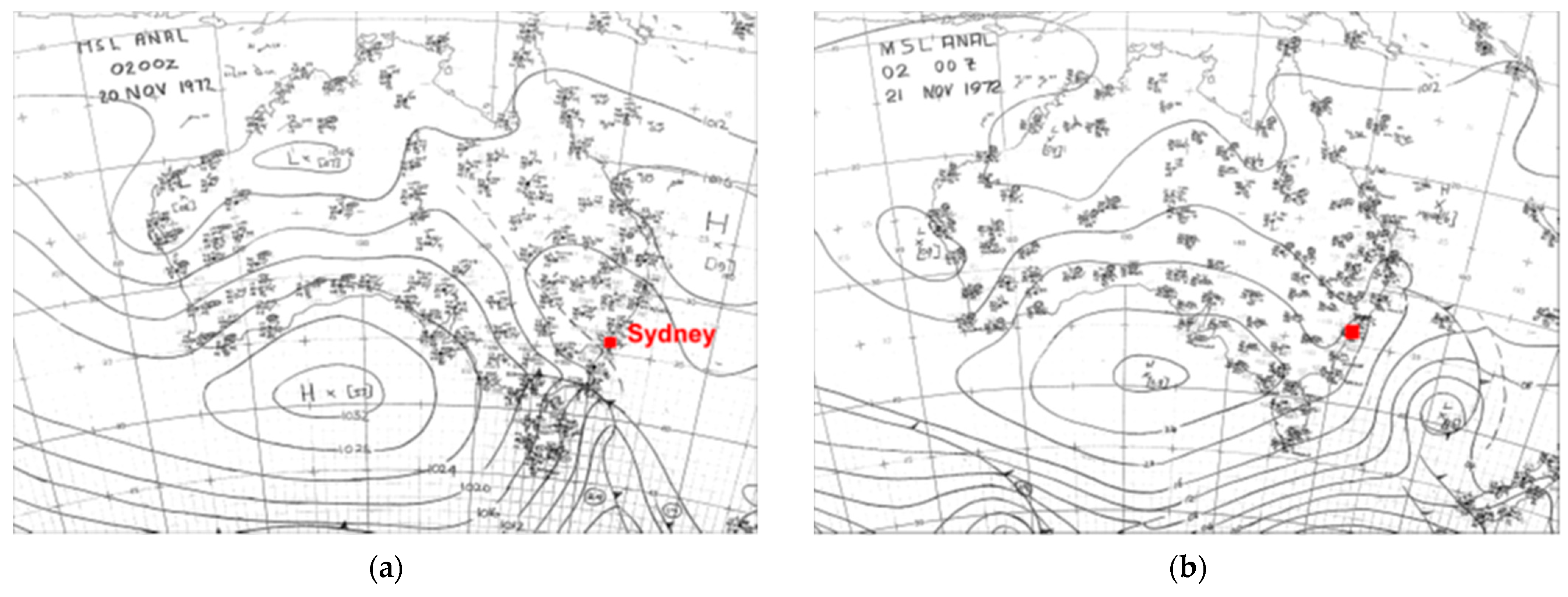
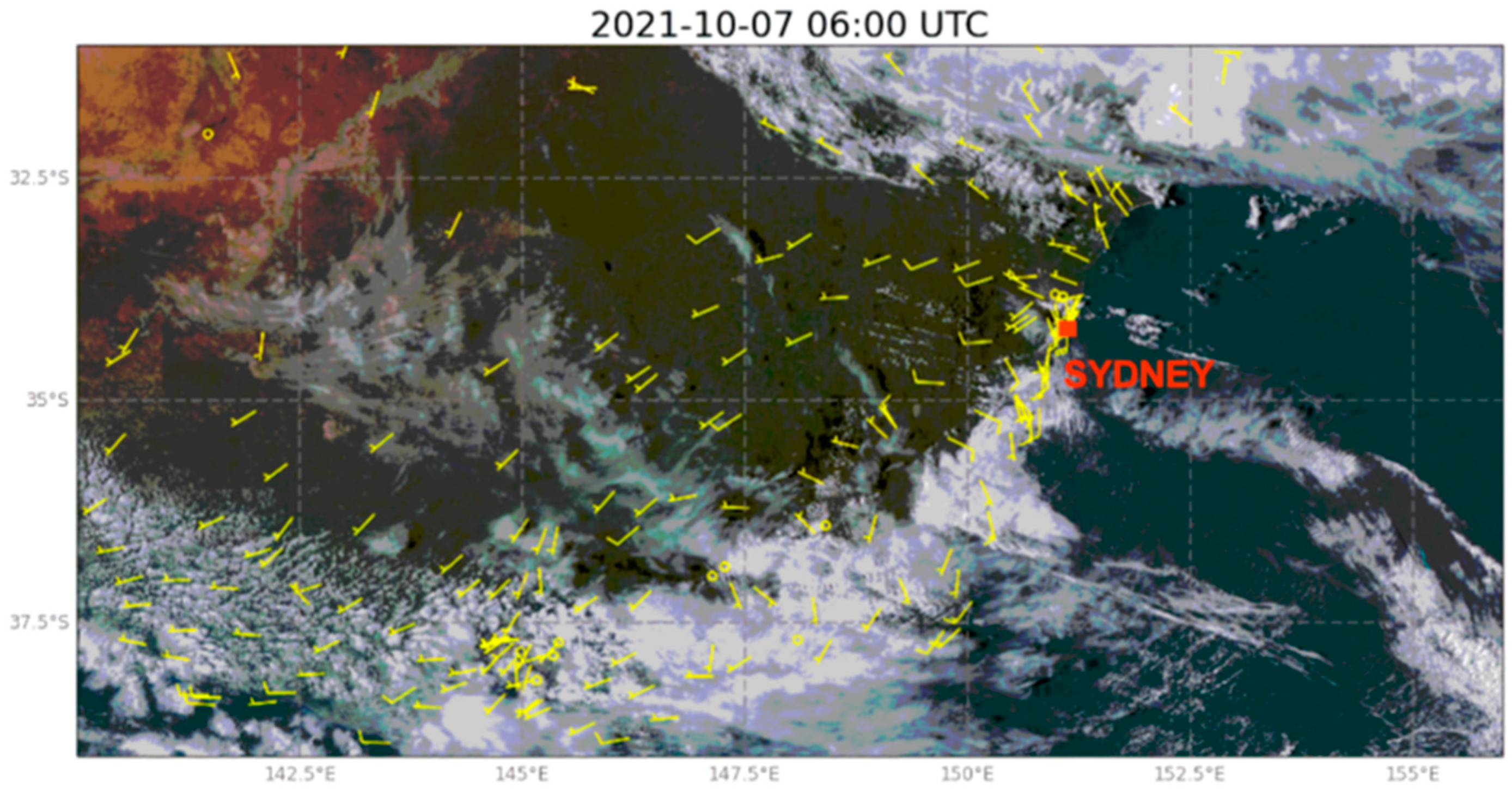
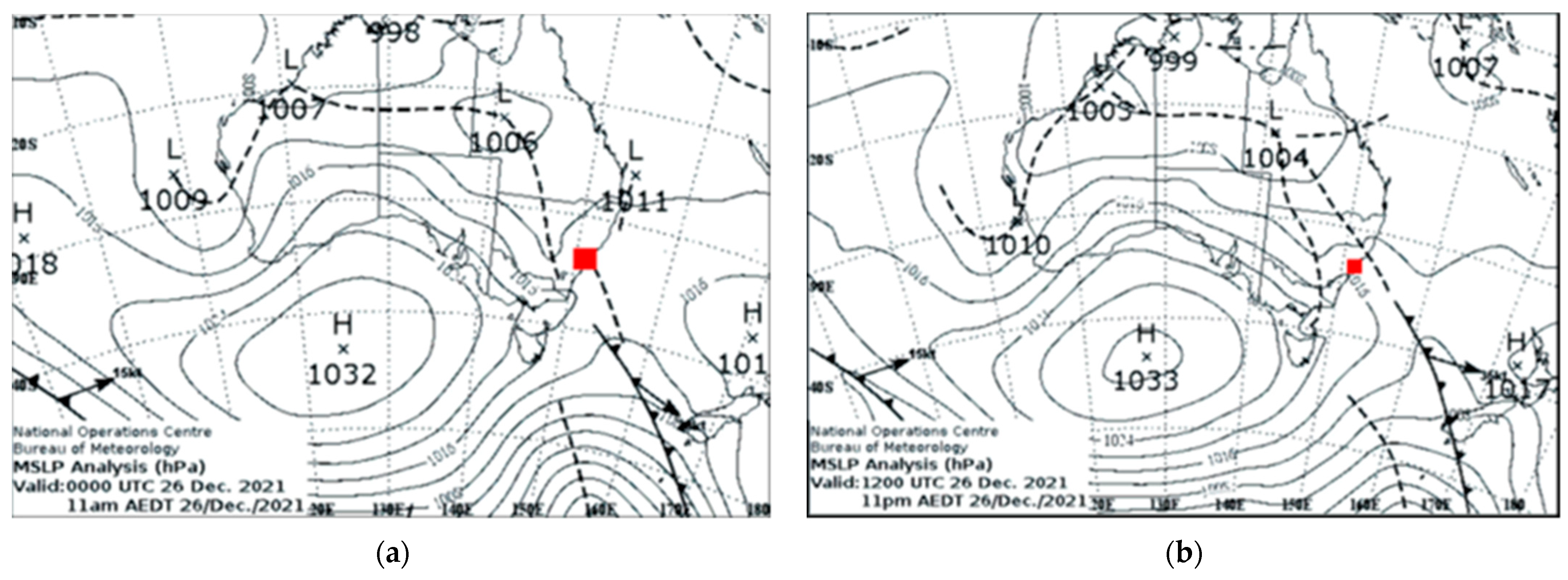
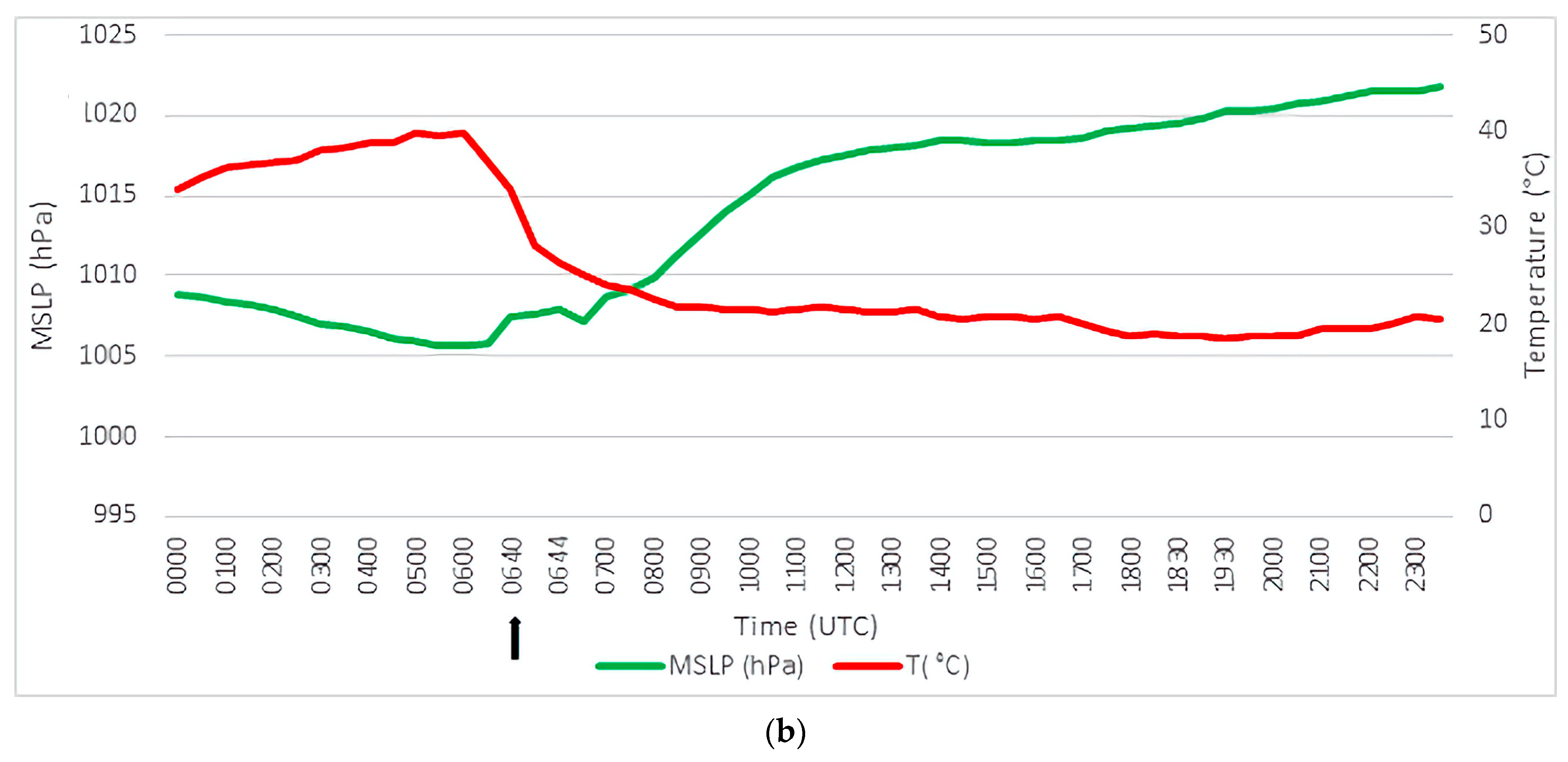
3.1.1. Examples of Southerly Busters before and during Accelerated GW

The SB example in Figure 1a,b above occurred in the period 1970–1971 to 1995–1996, representative of the period before accelerated GW when, typically, both SB and SSB maximum gust values in both El Niño and La Niña phases were significantly larger than in recent decades and particularly in recent years.

A more recent example in Figure 3a,b for 26 December 2021, below, occurred after the mid-1990s, within a period of statistically significant lower maximum gust speeds of both SBs and SSBs compared to the period prior to the mid-1990s. A common feature increasingly occurring after the mid-1990s compared to 1970–1971 to 1995–1996 is more zonal and weaker ridging from high-pressure centers in the GAB which is apparent on the Sydney coast in Figure 3b. With maximum gust speeds significantly decreasing after 1995–1996, it is possible that the weakened, zonal ridging is a sign of shallower, less dense air with less contrast in density ahead of the frontal system. This is explored in Section 3.2.

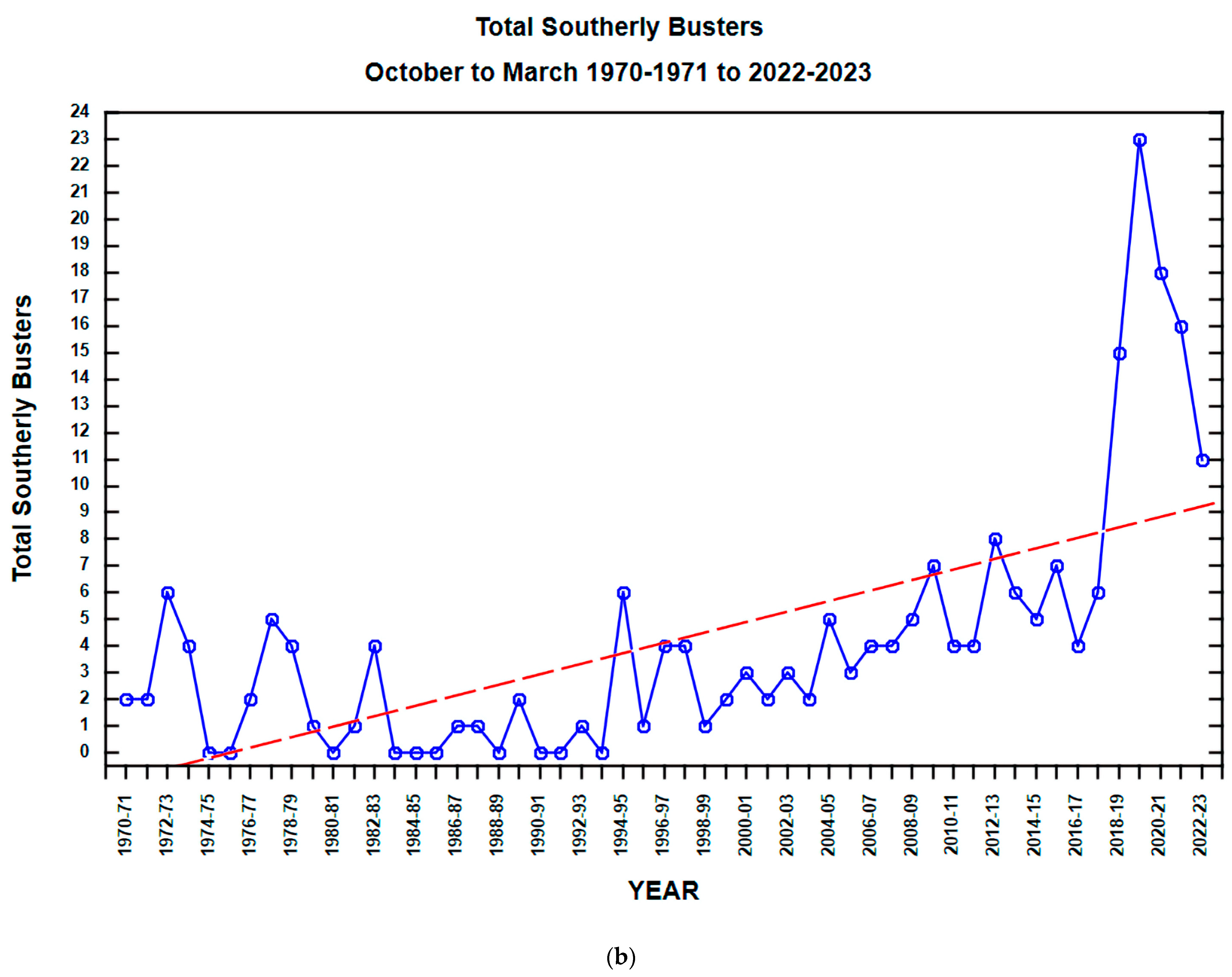
3.1.2. SB and SSB Frequencies October to March 1970–1971 to 2022–2023

Figure 4a shows that the annual frequency of SBs has increased steadily since the mid-1990s whereas the frequency of SSBs has stayed much the same. There were more SBs during El Niño phases prior to the mid-1990s as shown in 1972–1973, 1977–1978, 1982–1983, and 1994–1995. However, that relationship diminished after the mid-1990s with the main feature, apart from an overall increase in SBs, being a marked decrease in SBs and SSBs during the 2020–21 to 2022–23 triple La Niña phase. Similar to SBs, higher frequencies of SSBs dominated the El Niño years prior to the mid-1990s.

The annual frequencies of all SBs (SBs plus SSBs) reveal a steady increase which starts to occur in the mid-1990s (Figure 4b). That increase is clearly dominated by SBs as discussed at the start of Section 3.1.2. The main feature in Figure 4b is the very large increase, consisting of both SBs plus SSBs, for the years 2018–2019 and 2019–2020. These two spring–summer periods were extremely dry and warm in southeast Australia, with El Niño conditions especially during the core years of 2018 and 2019, likely giving a temporary boost to both SB and SSB annual counts. Then, in the following triple La Niña period 2020–2021 to 2022–2023, both SBs and SSBs annual counts both decreased.

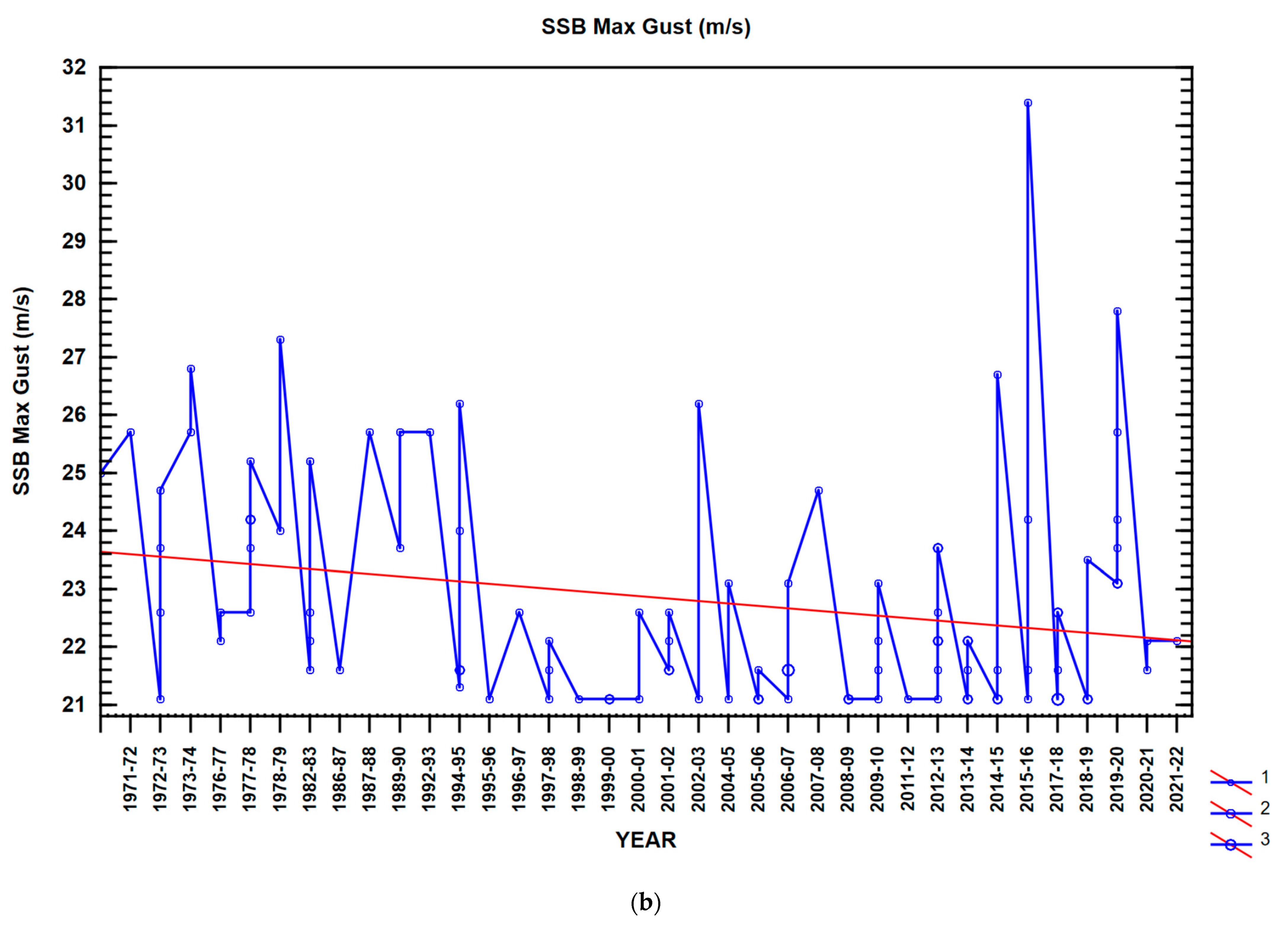
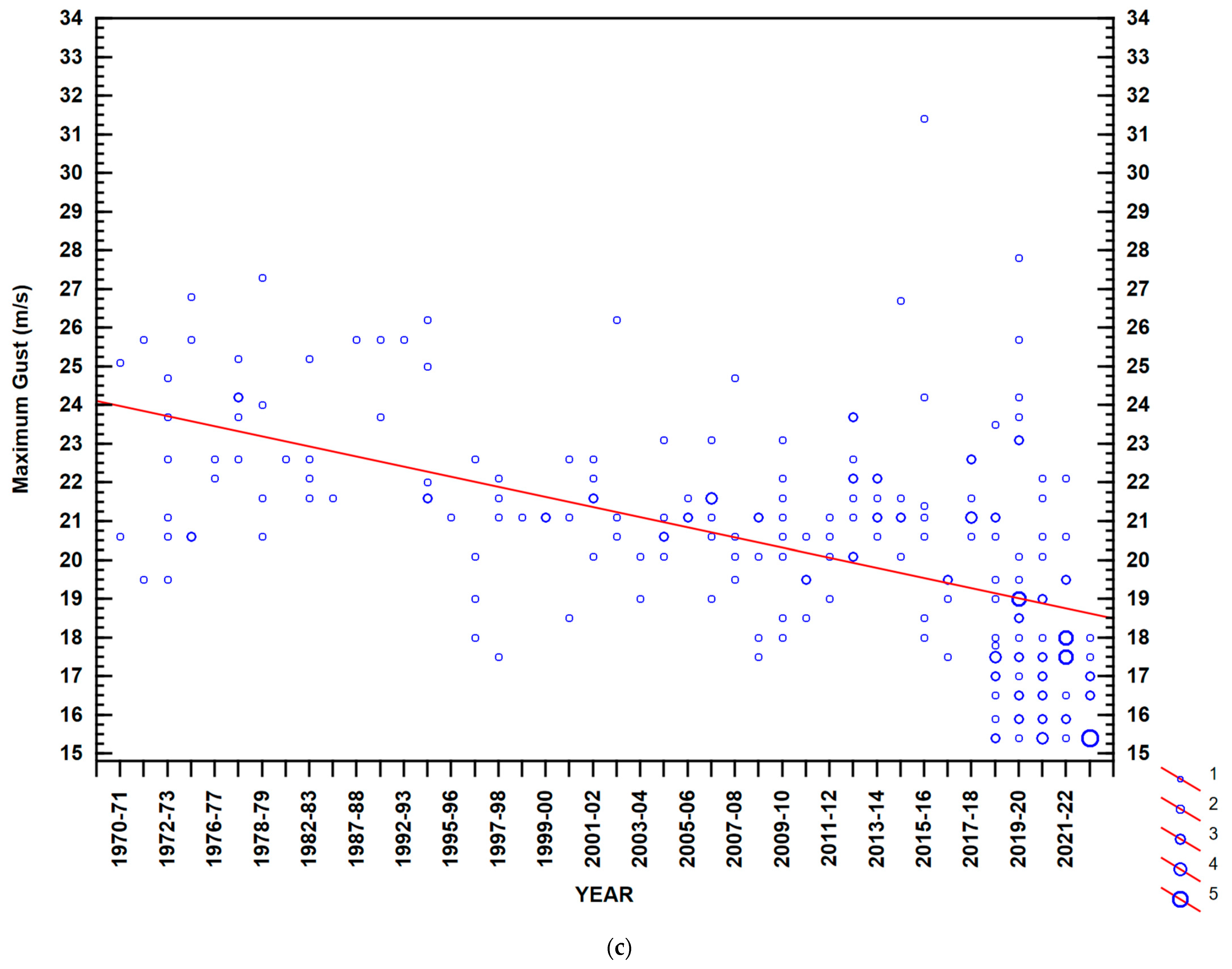
3.1.3. SB and SSB Maximum Wind Gust Values October to March 1970–1971 to 2022–2023

SBs are formally defined as wind gusts of at least 15 m/s and SSBs are defined as gusts of at least 21m/s [1]. There is a clear decreasing trend in maximum gust strength values of SBs along with their increasing frequency, which is evident from 2018–2019 (Figure 5a). Similarly, with SSBs (Figure 5b) there also is a decreasing trend in maximum values from the mid-1990s, with a noteworthy outlier at 31.4 m/s in 2015–16. Although maximum gust values of both SBs and SSBs have decreased, synoptic variability is inherent in mid-latitude frontal systems because the hemispheric scale Southern Annular Mode (SAM), which is a measure of the north–south movement of mid-latitude pressure systems [25], operates on a time scale of weeks. Hence, strong air pressure and density differences can potentially produce extreme maximum gusts in frontal systems (see Section 3.2). For SBs, the high variability is apparent throughout the entire period, but is most pronounced over the last decade. Variability in SSB maximum wind gusts also increases in the most recent decade.

A common feature increasingly occurring after the mid-1990s compared to 1970–1971 to 1995–1996 is weaker coastal ridging from high-pressure centers in the GAB, which is apparent in the SB in Figure 3a,b compared to the SB in Figure 1a,b. With maximum gust speeds significantly decreasing after 1995–1996 (Figure 5c), it is possible that the weakened, zonal ridging is a sign of shallower, less dense air with less contrast in density ahead of the frontal system. This is explored in Section 3.2.

3.1.4. Permutation Test for Differences in Mean Frequency of SBs and SSBs

A permutation test was carried out for the statistical significance of the differences in the means of the SBs and the SSBs of the October to March data between the two periods 1970–1971 to 1995–96 and 1996–1997 to 2022–2023 (

Table 1. SB, SSB, and total (SBs plus SSBs) mean frequency for the periods 1970–1971 to 1995–1996 and 1996–1997 to 2022–2023. p-values for difference between the two periods for both SBs and SSBs are also shown. Note that the difference in SB means for the two periods is highly significant (<1%) and for SSBs means the difference is significant (<10%). The increase in the total (SBs plus SSBs) is also highly significant (<1%).

Frequency	October to March 1970–1971 to 1995–1996	October to March 1996–1997 to 2022–2023	p-Value (between the Two Periods)
	Mean	Mean
SBs	0.3	4.4	0.004
SSBs	1.6	2.3	0.07
Total (SB plus SSB)	1.7	6.6	0.002

). The means for the two periods were 0.3 and 4.4 SB events/year, and 1.6 and 2.3 SSB events/year, respectively. The permutation test without replacement was applied to test the null hypothesis that the mean frequencies of the two time series periods were not significantly different. The permutation test yielded a p-value of 0.004 for the SBs and 0.07 for the SSBs. For total SB plus SSB events/year it is 1.7 and 6.6 with p-value 0.002. The finding that the frequency of SBs had increased significantly, but not for the SSBs, was unsurprising from an inspection of the time series in Figure 4a,b.

3.1.5. MSLP Characteristics of Southerly Busters Related to ENSO Phases

SBs and SSBs occur during all ENSO phases; El Niño, La Niña, and neutral. In

Table 2. (a) Average frequency of SBs and SSBs for the total period 1970–1971 to 2022–2023. The numerator is the number of SBs or SSBs and the denominator is the number of phases. (b) Average frequency of SBs and SSBs for the two split periods 1970–1971 to 1995–1996 and 1996–1997 to 2022–2023. The numerator is the number of SBs or SSBs and the denominator is the number of phases.

(a)
ENSO Phase	ENSO Phase
	SB Average		SSB Average
La Niña	(61/17) = 3.6		(19/17) = 1.5
El Niño	(8/13) = 0.6		(37/13) = 2.8
Neutral	(46/23) = 2		(42/23) = 1.8
(b)
ENSO Phase	SB Average		SSB Average
	1970–1971 to 1995–1996	1996–1997 to 2022–2023	1970–1971 to 1995–1996	1996–1997 to 2022–2023
La Niña	(4/6) = 0.7	(57/11) = 5.2	(4/6) = 0.7	(17/6) = 2.8
El Niño	(2/8) = 0.3	(10/5) = 2.0	(22/8) = 2.8	(15/5) = 3.0
Neutral	(1/12) = 0.1	(41/11) = 3.7	(13/12) = 1.1	(30/11) = 3.0

a and Table 2b, respectively, they are averaged in each phase for the total period 1970–1971 to 2022–2023 and the two split periods 1970–1971 to 1995–1996 and 1996–1997 to 2022–2023. The ENSO phases are defined according to the Australian Bureau of Meteorology (http://www.bom.gov.au/climate/history/enso/ (accessed on 24 June 2024)). Note the marked preference for SBs to occur in La Nina phases over the period 1970–1971 to 2022–2023 (Table 2a). SBs rarely occurred before the early–mid-1990s (Figure 4a). The increase in SBs from the mid-1990s can be attributed primarily to a large increase in numbers during the triple La Nina phase 2020–2023. In contrast, SSBs appear most frequently during El Nino phases. In El Nino phases, the difference in air density ahead of the SSB, compared to just after the SSB passage, is likely to be larger than for an SB because of the cooler SSTs near the southeast Australian coast, given the same air temperature because of the relationship of air density with temperature and pressure in the equation of state.

When the SB and SSB frequencies are split into the periods before and during accelerated GW, there is a marked difference in their frequency links to ENSO phases (Table 2b). The SB frequency is much higher in La Nina phases in the accelerated GW period than in the prior period, owing mainly to the large number of SBs in the 2020–2023 triple La Niña and the lack of SBs in the first period, as discussed above. However, the frequencies of both SBs and SSBs show a preference for La Nina and neutral phases in the accelerated GW period, but little difference in preference for the El Nino phase between the two time periods. For SSBs, the likely cause for little change in preference for the El Niño phase between the two time periods is the synoptic variability of frontal systems not affecting the frequency of SSBs, even after changes in the global and local atmospheric circulation have occurred. This is explored further in the next section.

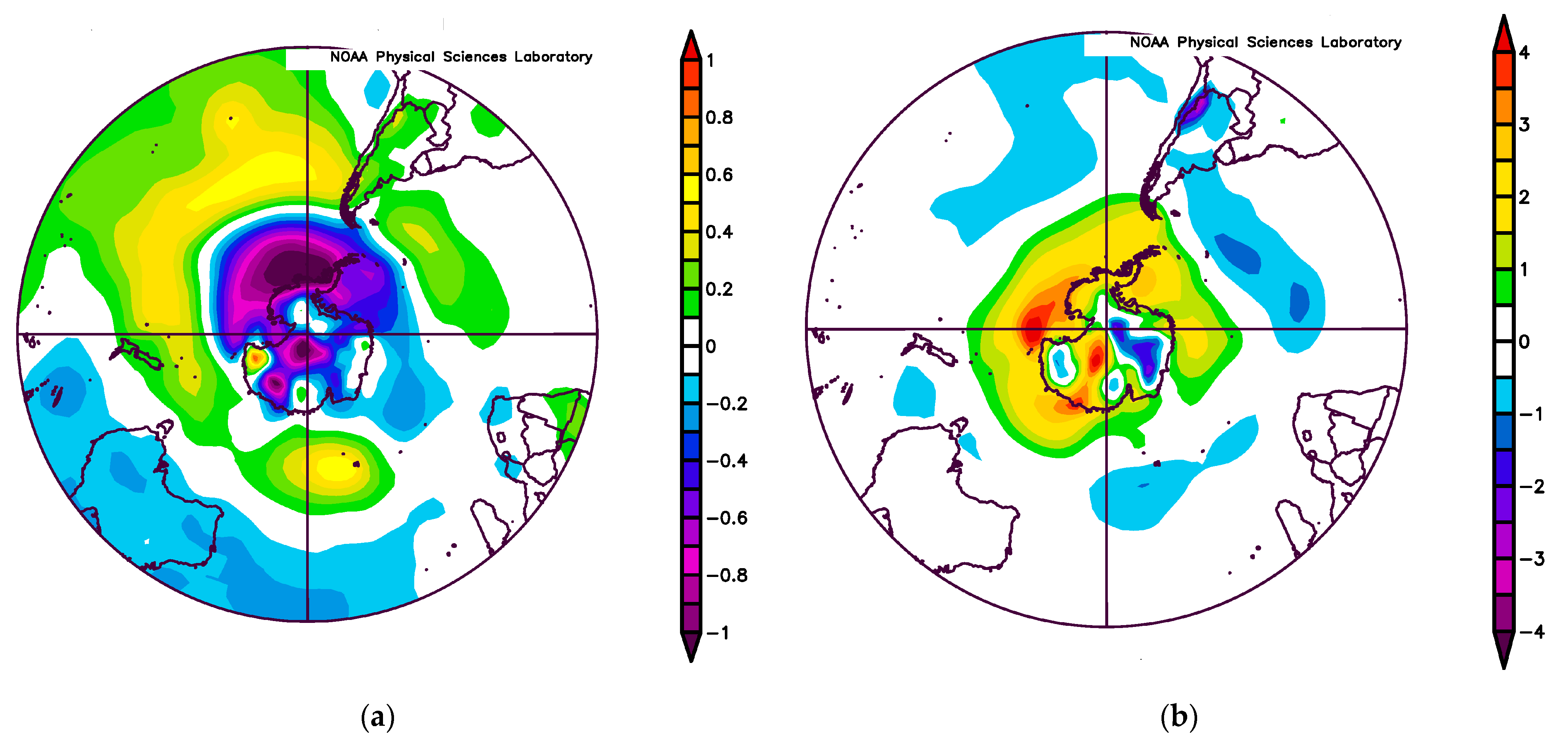
3.2. Global and Local General Circulation Changes

3.2.1. Impact on SBs and SSBs of Changes in the Global and Local General Circulation

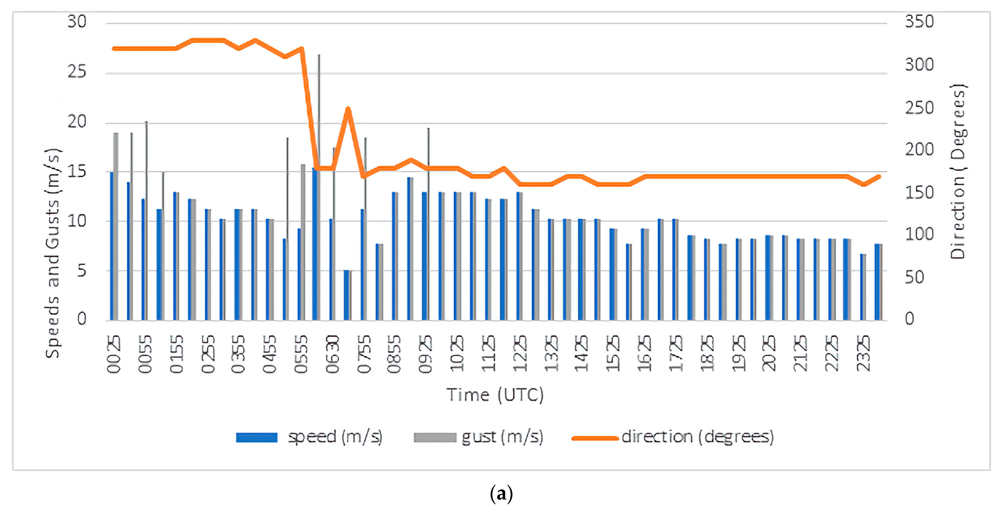
On the hemispheric scale, it is possible to identify changes in MSLP values south of the Australian continent, where SBs and SSBs develop, suggesting a link to changes in synoptic features of the frontal systems that spawn SBs and SSBs. Figure 6 indicates that at latitudes immediately south of the Australian continent, anomalous high pressure from 1996–1997 to 2022–2023 has replaced weakly, anomalous low pressure from 1970–1971 to 1995–1996 with continental land-based low-pressure anomalies from 1996–1997 to 2022–2023 indicative of anomalous heating over land (Figure 6a and Figure 6b, respectively). These SH circulation changes are characteristic of SAM, briefly mentioned in Section 3.1.1 in relation to gust strength. Figure 6a implies that in the latter period when the ever-present well-defined circumpolar vortex around Antarctica extends its zonal westerly winds into the mid-latitudes south of Australia in the form of cold frontal systems emanating from the polar front jet, the zonal high-pressure anomalies just south of the Australian continent favor zonal high-pressure ridging with weak zonal pressure gradients on the synoptic scale because the cold, dense air is too far poleward. That persistent SH circulation feature from October to March has enabled increased coastal ridging, more often in the form of SBs, than in the early period. In the early period, high-pressure anomalies over Antarctica imply outflowing very cold, dense air which can be captured only occasionally by mid-latitude frontal systems south of the Australian continent.

Synoptically, the typical sequence, irrespective of the ENSO phase, is for high pressures over the Tasman Sea to direct warm-to-hot N/NW winds over the southeast Australian coast ahead of a Southern Ocean frontal system moving from west to east. The frontal system introduces a much cooler, denser air mass which travels much faster through Bass Strait due to less friction than further north over land. On MSLP synoptic charts this appears as a ridge of high pressure extending from a high-pressure center in the GAB or farther west. Once the colder, denser air behind the frontal system reaches eastern Bass Strait it turns northward, and the ridging continues parallel to the coast as a density current trapped by the GAB to the west of the coastal plain in the manner described by [3,4,5,6,7].

3.2.2. SSB Examples

Two SSB examples illustrate how the atmospheric environments in which they formed differ between the two periods 1970–1971 to 1995–1996 and 1996–1997 to 2022–2023. The examples are from 20 November 1973, and 31 January 2019, respectively. Both are SSBs, because their maximum wind gusts exceed 21 m/s during the passage of the SB, as shown in the recorded maximum wind gusts in Figure 7a and Figure 8a. In addition, both wind directions change from about 330 degrees (NW) to 200 degrees, respectively, prior to and after the SSB passage.

However, the environments for the two SSBs differ markedly, as shown in Figure 7b and Figure 8b. In Figure 7b, the MSLP rises from 1000 hPa to about 1015 hPa before and after the SSB passage. Also, in Figure 7b, the screen temperature drops from around 33 °C to about 18 °C. In Figure 7b, the corresponding pressure rise is from 1008 hPa to 1022 hPa. The temperature drops from 41 °C to 22 °C.

The SSBs in 1973 and 2019 formed in highly contrasting environments but had very similar pressure rises of 15 and 14 hPa, respectively, following the SSB passage, but a larger temperature decrease of 19 °C in the 2019 case compared with 15 °C in the 1973 case.

4. Discussion

In this study, the iconic Southerly Buster (SB) which affects coastal southeast Australia is assessed to be strongly impacted by the accelerated global warming (GW) that has occurred since the early–mid 1990s. To the best of our knowledge, this is the first time that characteristics of southerly busters have been investigated in relation to global warming. The impacts have involved the amplification by GW in certain phases of several of the key climate drivers influencing southeastern Australia, most notably ENSO and SAM. In the first period, 1970–1971 to 1995–1996, SBs are dominated by either neutral or La Niña phases and SSBs are dominated by neutral or El Niño phases. In the second period, 1996–1997 to 2022–2023, SSBs are likely in any ENSO phase, owing to synoptic variability even after changes that have occurred in the SH circulation.

The southeastern Australian coastal region warm season, defined here as the six months October to March, was divided into two consecutive periods, the pre-accelerated GW years 1970–1971 to 1995–1996 and the accelerated GW years 1996–1997 to 2022–2023. The annual frequency counts of SBs and strong SBs (SSBs) showed a clear change between SSBs dominating the first period, whereas SBs are far more prevalent than SSBs in the second period. There is an increasing trend in the annual frequencies of SBs and a marginally increasing trend in the frequencies of SSBs over the entire period 1970–1971 to 2022–2023. Given the definitions of maximum gust thresholds for SBs and SSBs and the larger increase in SBs than SSBs, it is not surprising that there is a decreasing trend in the maximum wind gusts of the total SBs and SSBs during 1970–1971 to 2022–2023.

An explanation for the observed frequency changes in SBs and SSBs is related to the influence on SAM of changes in the general circulation, and in the local circulation consequences, during the accelerated GW period. These SH circulation changes, which are mainly due to positive SAM, imply that in the latter period when the ever-present well-defined circumpolar vortex around Antarctica extends its zonal westerly winds into the mid-latitudes south of Australia in the form of cold frontal systems emanating from the polar front jet, the zonal high-pressure anomalies just south of the Australian continent favor zonal high-pressure ridging with weak zonal pressure gradients on the synoptic scale because the coldest, most dense air is too far poleward in the polar vortex. That persistent SH circulation feature from October to March has enabled increased coastal ridging, more often in the form of SBs, than in the early period. In the early period, high-pressure anomalies over Antarctica (Figure 5b) imply outflowing very cold, dense air can be captured, albeit only occasionally, by mid-latitude frontal systems south of the Australian continent.

Owing to the increase in SBs, the implications for marine and aviation safety are clearly important. The many surfing beaches on the coastline of southeast Australia, which experiences SBs from October to March, are frequently crowded with people and small watercraft, while the low-level wind shear associated with increased SBs at coastal airports can enhance the danger to aircraft while taking off and landing. Another very important implication of increasing SBs is the associated sudden changes in wind direction which increase the danger when bushfires are present.

Tropospheric circulation changes induced by global warming have been responsible for the increase in SBs. However, assuming continued global warming, it is uncertain the extent to which further increases will occur. That scenario could benefit from a climate modelling study that takes into account tropospheric circulation changes.

References

1. Colquhoun, J.R.; Shepherd, D.J.; Coulman, C.E.; Smith, R.K.; McInnes, K. The Southerly Burster of South Eastern Australia: An Orographically Forced Cold Front. Mon. Wea. Rev. 1985, 113, 2090–2107. [Google Scholar] [CrossRef]
2. Gentilli, J. Some regional aspects of southerly buster phenomena. Weather 1969, 24, 173–184. [Google Scholar] [CrossRef]
3. Baines, P.G. The Dynamics of the Southerly Buster. Aust. Meteorol. Mag. 1980, 28, 175–200. Available online: http://www.bom.gov.au/jshess/docs/1980/baines.pdf (accessed on 24 April 2024).
4. Mass, C.E.; Albright, M.D. 1987: Coastal southerlies and alongshore surges of the west coast of North America: Evidence of mesoscale topographically trapped response to synoptic forcing. Mon. Wea. Rev. 1987, 115, 1707–1738. [Google Scholar] [CrossRef]
5. Egger, J.; Hoinka, K.P. Fronts and orography. Meteorol. Atmos. Phys. 1992, 48, 3–36. [Google Scholar] [CrossRef]
6. McInnes, K.L. Australian southerly busters. Part III: The physical mechanism and synoptic conditions contributing to development. Mon. Wea. Rev. 1993, 121, 3261–3281. [Google Scholar] [CrossRef]
7. Reid, H.; Leslie, L. Modeling coastally trapped wind surges over southeastern Australia. Part I: Timing and speed of propagation. Weather Forecast. 1999, 14, 53–66. [Google Scholar] [CrossRef]
8. Australian Bureau of Meteorology. Hazards, Warnings and Safety. Available online: http://www.bom.gov.au/marine/knowledge-centre/hazards.shtml (accessed on 24 April 2024).
9. Holland, G.J.; Leslie, L.M. Ducted coastal ridging over S.E. Australia. Q. J. R. Meteorol. Soc. 1986, 112, 731–748. [Google Scholar] [CrossRef]
10. Gill, A.E. Coastally trapped waves in the atmosphere. Quart. J. Roy. Meteor. Soc. 1977, 103, 431–440. [Google Scholar] [CrossRef]
11. Reason, C.J.C. Orographically trapped disturbances in the lower atmosphere: Scale analysis and simple models. Meteorol. Atmos. Phys. 1994, 53, 131–136. [Google Scholar] [CrossRef]
12. Reason, C.J.C.; Steyn, D.G. Coastally trapped disturbances in the lower atmosphere: Dynamic commonalities and geographic diversity. Prog. Phys. Geogr. Earth Environ. 1990, 14, 178–198. [Google Scholar] [CrossRef]
13. Reason, C.J.C.; Steyn, D.G. The Dynamics of Coastally Trapped Mesoscale Ridges in the Lower Atmosphere. J. Atmos. Sci. 1992, 49, 1677–1692. [Google Scholar] [CrossRef]
14. Reason, C.J.C.; Tory, K.J.; Jackson, P.L. Evolution of a Southeast Australian Coastally Trapped Disturbance. Meteorol. Atmos. Phys. 1999, 70, 141–165. [Google Scholar] [CrossRef]
15. Available online: https://www.smh.com.au/national/nsw/sydney-s-defining-weather-event-is-back-but-why-did-southerly-busters-go-awol-20231018-p5ed74.html (accessed on 24 April 2024).
16. Australia State of the Environment 2016: Built Environment. Available online: https://soe.dcceew.gov.au/sites/default/files/2022-05/soe2016-built-launch-20feb.pdf (accessed on 24 June 2024).
17. Bubathi, V.; Leslie, L.; Speer, M.; Hartigan, J.; Wang, J.; Gupta, A. Impact of Accelerated Climate Change on Maximum Temperature Differences between Western and Coastal Sydney. Climate 2023, 11, 76. [Google Scholar] [CrossRef]
18. BoM 2020. Australian Bureau of Meteorology and CSIRO. State of the Climate 2020. Available online: https://bom.gov.au/state-of-the-climate/ (accessed on 14 June 2024).
19. IPCC. Contribution of Working Group I to the Sixth Assessment Report of the Intergovernmental Panel on Climate Change. In Climate Change 2021: The Physical Science Basis; Masson-Delmotte, V., Zhai, P., Pirani, A., Connors, S.L., Péan, C., Berger, S., Eds.; Cambridge University Press: Cambridge, UK; New York, NY, USA, 2021; Available online: https://www.ipcc.ch/report/ar6/wg1/downloads/report/IPCC_AR6_WGI_SPM_final.pdf (accessed on 24 June 2024).
20. NOAA. National Centers for Environmental Information, State of the Climate: Global Climate Report for 2019. Available online: https://www.ncdc.noaa.gov/sotc/global/201913/supplemental/page-3 (accessed on 14 June 2024).
21. Speer, M.S.; Leslie, L.M.; MacNamara, S.; Hartigan, J. From the 1990s climate change has decreased cool season catchment precipitation reducing river heights in Australia’s southern Murray-Darling Basin. Sci. Rep. 2021, 11, 16136. [Google Scholar] [CrossRef] [PubMed]
22. Speer, M.; Hartigan, J.; Leslie, L. Machine Learning Assessment of the Impact of Global Warming on the Climate Drivers of Water Supply to Australia’s Northern Murray-Darling Basin. Water 2022, 14, 3073. [Google Scholar] [CrossRef]
23. Speer, M.; Leslie, L.; Hartigan, J.; MacNamara, S. Changes in Frequency and Location of East Coast Low Pressure Systems Affecting Southeast Australia. Climate 2021, 9, 44. [Google Scholar] [CrossRef]
24. Australian Bureau of Meteorology ENSO Phases. Available online: http://www.bom.gov.au/climate/history/enso/ (accessed on 24 April 2024).
25. The Southern Annular Mode. Available online: http://www.bom.gov.au/climate/enso/#tabs=Southern-Ocean&southern=History (accessed on 24 April 2024).
Figure 1. Australian Bureau of Meteorology mean sea level pressure (MSLP) archived analysis showing contours of manually plotted observations, (a) at 0200 UTC 20 November 1972, before the SB passage, (b) at 0200 UTC 21 November 1972, after the SB passage. The wind direction changes from northwesterly in Sydney (left panel), to southerly (right panel) as the ridging moves up the east coast.
Climate 12 00096 g001
Figure 2. Himawari-8 satellite at 0600 UTC, 7 October 2021, showing satellite-derived wind vectors close to the surface. Note the marked delineation between NW winds before the SB and southerly winds after the passage of the SB at the coast through Sydney. Half-length yellow wind barbs indicate from 3 to 7 knots and full-length wind barbs indicate from 8 to 12 knots.
Climate 12 00096 g002
Figure 3. Mean sea level pressure (MSLP) analysis, (a) on 26 December 2021 00 UTC, before the SB passage, (b) on 26 December 2021 12 UTC, after the SB passage. The wind direction changes from northwesterly in Sydney (left panel), to southerly (right panel).
Climate 12 00096 g003
Figure 4. (a) SB and SSB frequencies October to March 1970–1971 to 2022–2023. Blue and red lines are the SBs and SSBs, respectively. Blue and red dashed lines represent the linear trends in the SBs and SSBs. Note the steady increase in SBs from the mid-1990s. (b) Frequency of all SBs (SBs plus SSBs) October to March 1970–1971 to 2022–2023. Frequency is indicated by open, blue circles. The dashed red line is the linear trend.
Climate 12 00096 g004aClimate 12 00096 g004b
Figure 5. (a) The 1970–1971 to 2022–2023 frequency distribution of SB maximum gust strength values (15.0–20 m/s). Increasing numbers of the same maximum gust strength value within an October to March period are shown by the increasing size of the open circles, enumerated in the legend. (b) The 1970–1971 to 2022–2023 frequency distribution of SSB maximum gust strength values (21.0–maximum recorded value, m/s). Increasing numbers of the same maximum gust strength value within an October to March period are shown by the increasing size of the open circles, enumerated in the legend. (c) The 1970–1971 to 2022–2023 total frequency distribution of maximum gust strength values (21.0–maximum recorded value, m/s). Increasing numbers of the same maximum gust strength value within an October to March period are shown by the increasing size of the open circles, enumerated in the legend.
Climate 12 00096 g005aClimate 12 00096 g005bClimate 12 00096 g005c
Figure 6. (a) Southern Hemisphere NOAA/PSL MSLP anomalies (hPa) October to March 1997–2023, (b) South Hemisphere NOAA/PSL MSLP anomalies (hPa) October to March 1971–1996.
Climate 12 00096 g006
Figure 7. (a) Shows the 30 min plots of wind speeds (m/s, blue lines) and wind gusts (m/s, grey lines) for the passage of the southerly buster through Sydney on 20 November 1973. The orange line is the wind direction in degrees. The maximum wind gust is 27 m/s at approximately 0600 UTC. (b) Shows the 30 min plots of MSLP (green line) and temperature (red line) for the passage of the southerly buster through Sydney on 20 November 1973. The precise passage time is shown by the vertical black arrow at approximately 0600 UTC.
Climate 12 00096 g007aClimate 12 00096 g007b
Figure 8. (a) Shows the 30 min plots of wind speeds (m/s, blue lines) and wind gusts (m/s, grey lines) for the passage of the southerly buster through Sydney on 31 January 2019. The orange line is the wind direction in degrees. The maximum wind gusts of about 23–25 m/s occurred during the period at approximately 0645–0900 UTC. (b) Shows the 30 min plots of MSLP (green line) and temperature (reed line) for the passage of the southerly buster through Sydney on 31 January 2019. The precise passage time is shown by the vertical black arrow at approximately 0640 UTC.
Climate 12 00096 g008aClimate 12 00096 g008b