1. Introduction
As a consequence of rising global average temperatures due to increasing atmospheric greenhouse gas concentrations and other forcing factors, an increase in extreme temperature events is likely in some regions of the world [
1,
2]. Recent published studies have shown that the number of warm anomalies in the climate system is changing [
3]. Extremely hot days and nights will likely become more frequent and extreme cold days and nights less frequent [
4]. Nevertheless, in 2013 the winter in Central Europe ended unusually late leading to freezing temperatures accompanied by lasting snow cover [
2]. Extreme temperature events are recorded in the Emergency Events Database (EM-DAT) if one of the following conditions is fulfilled: Ten or more people reported killed, one hundred or more people reported affected, declaration of a state of emergency, or call for international assistance. Song
et al. [
5] used data on the frequency and the number of fatalities from EM-DAT and analysed their temporal trends and spatial patterns from 1981 to 2010 at the global scale. Over these three decades, the frequencies of heat waves reported by EM-DAT increased by a factor of 2.7 and cold spells by 6.4 per decade since the 1980s, with a large regional variability. More than 40% of the extreme events recorded in the database occurred in Europe [
5].
These recent studies raise the question as to whether the temporal scales of variability of temperature data have changed measurably in the recent past. This requires first and foremost a consideration of statistical methods to analyse the statistical properties of climate time-series data. In particular, it raises the question as to whether changes in temporal scales can be adequately described by “traditional” statistics such as the mean, standard deviation or frequency of events. It is known from spatio-temporal theory that observing a process at the wrong temporal scale can lead to patterns remaining undetected [
6].
In the global climate system, temporal scales of variability are of paramount importance, and many studies in the climatological literature have described various climatic oscillations and teleconnections. The analysis of the temporal scales of variability of several climate indices with continuous wavelet analysis showed a common shift in the frequency structure around 1970, affecting decadal and multi-decadal scales for all climate indices: Atlantic Multidecadal Oscillation (AMO), the North Atlantic Oscillation (NAO), the Northern Annular Mode (NAM), the Pacific Decadal Oscillation (PDO), the Southern Oscillation Index (SOI) and the Pacific-North-America teleconnection (PNA) [
7]. The total variance of the climate indices showed a common distribution in time, which is interpreted as “a more or less ‘connected’ evolution” of the total variance over time [
7]. Averaging the AMO, PDO, SOI and NAO indices showed that during 1930–1960 and 1980–2000 the variance was high and during 1960–1980 it was low [
7].
The current study investigates a new method for the statistical analysis of temporal scales of variability in climate time-series data. We describe the first statistical analysis of a climatological temperature record with MSE analysis. MSE is based on the estimation of the sample entropy [
8] of the time-series after coarse-graining at different temporal scales. Its principle is that systems of higher complexity tend to generate responses that appear to be more random or less ordered than low-complexity systems [
9]. System complexity is a notion that has been defined in different ways in the literature. Intuitively, it is clear that a system that consists of only one simple deterministic process has low complexity. Equally, a system that is pure white noise can be represented by only one equation and is considered structurally simple (not complex), but it is not predictable. Even deterministic systems can be very poorly predictable from observations if their complexity leads to the amplification of small disturbances. The complexity of a system that is measured by a time-series of observations becomes important to characterize in order to determine its predictability. A review of the literature on the topic of complexity [
10] concludes that the word “complexity” is used either as a “quality whose attributes characterize all complex systems”, or as a “quantitative measure that characterizes a system, thus capturing the notion that some systems (mathematical or physical) are more or less complex than others”. In that paper, Bar-Yam [
10] defines a notion of “descriptive complexity” by stating that “the complexity of a system is related to the length of its shortest description”. For example, in climate science, the description of the climate system can be a physical climate model or an empirical model. It is clear that the more complex the climate system is in reality, the longer the algorithmic description of the climate processes in the climate model has to become.
Our definition of “complexity” in this paper is quantitative and based on entropy. The MSE plots are used to compare the relative complexity of normalized time-series and are interpreted as follows. Following Costa
et al.’s [
11] definition, if “[…] for the majority of the scales the entropy values are higher for one time-series than for another, the former is considered more complex than the latter”.
The MSE method was originally developed for diagnosing fluctuations of the human heartbeat in cardiology [
11]. In the cardiological study by Costa
et al. [
11], a loss of complexity at longer time-scales, which was apparent as lower entropy, was associated with ageing of patients and certain types of heart disease. More recently, MSE has been applied to hydrological data [
9,
12,
13] but it has not been used to analyse changes in the temporal scaling behaviour of temperature data to date. For example, an MSE analysis of a time-series of 131 years of daily flow rates of the Mississippi River revealed that sample entropy decreases over large time scales, indicating that the Mississippi river flow may have been losing complexity since the 1940s due to significant human land use change [
9].
From the above examples of applications of MSE it is clear that this method offers a deeper understanding of the properties of a time-series beyond what can be achieved with other more traditional analysis techniques. The present study therefore investigates whether MSE analysis can be applied to surface air temperature anomalies over Europe in order to test whether they have changed in their temporal complexity in the last 50 years compared to the long-term average. Regional temperatures are an expression of multiple climate forcing processes acting on different time-scales, including changing greenhouse gas concentrations, dynamic atmospheric pressure profiles, the mode of the North Atlantic Oscillation (NAO) and other regional climate patterns, fluctuations in solar irradiation and cloud dynamics. Because many of these processes have experienced significant changes, this study tests whether the complexity of the regional temperature time-series data, which can be seen as an expression of the underlying processes in the climate system, shows any evidence of changes at particular time-scales. It is the first application of MSE to air temperature anomaly data and tests the hypotheses that:
H1: Regional temperature anomalies in Europe show particular time-scales with higher or lower sample entropy than expected under the assumption of white noise, i.e., there are signals in the time-series that are only apparent at specific time-scales.
H2: The sample entropy of European temperature anomalies shows significant differences at particular time-scales when comparing 1851–1960 with 1961–2014, i.e., the temporal scaling properties of the temperature data have changed at specific temporal scales of observation.
2. Methods
Multi-scale entropy (MSE) is based on the estimation of the entropy of an observed time-series at different granularity. This is achieved by successively coarse-graining the original time-series data into new coarser scale time-series and re-analysing their entropy. By plotting the entropy estimates against the temporal scaling parameter (the degree of coarse-graining), the effect of scale on the regularity of patterns in the data can be effectively visualized. A detailed description of the MSE method can be found in [
11].
In information theory, the entropy of a random variable (such as time-series data) is a measure of its average uncertainty. Its origin is the Shannon entropy [
14], which quantifies the average unpredictability in a random variable, which is thus equivalent to its information content. The higher the entropy the lower the information content of the time-series. In information theory, the Shannon entropy
H(X) of a discrete random variable
X is calculated by the equation:
where
X is a random variable with probability mass function
p(
xi), θ is the set of all values
xi that
X can assume with
p(
xi)
> 0, and E is the expectation operator. A special case of
p log(
p) = 0 is defined if
p = 0.
For the analysis of a one-dimensional discrete time-series of
N measurements, [
x1, …,
xi, …,
xN], we first construct consecutive coarse-grained time-series, [
yτ(τ)], for different values of the temporal scale factor, τ. First, we divide the original times series into non-overlapping windows of length
τ, trimming any residual < τ elements at the end of the time-series. Second, we average all data points inside each window. The resulting coarse-grained time-series elements are calculated as:
for 1 ≤
j ≤
N/τ.
For scale τ = 1, the coarse-grained time-series (y(τ)) is identical to the original time-series. For τ > 1, each coarse-grained time-series contains elements, i.e., the length of the original time-series divided by the scale factor (omitting the remainder of the time-series with <τ elements). In the last step, we estimate the sample entropy for each coarse-grained time-series (y(τ)) and plot it against the scale factor τ.
Let us assume that the state of the parameter of interest at time
t + 1 is partially determined by its previous values at times
t −
m, …,
t − 1,
i.e., that it can be described by a state vector of length
m:The number of embedded state vectors within a Euclidean distance from some reference state is known in non-linear time-series analysis of dynamical systems as the local contribution to the classical correlation sum [
15]. Entropy for a time-series is defined as growth in unpredictability when increasing the length of the state vectors from
m to
m + 1. The effect that this change has is assessed by considering the statistical ensemble of all such states. In detail, for each vector
um(
i) of length
m, we count the number of vectors in the time-series that are similar to it,
i.e., that lie within a certain small distance that is proportional to the tolerance parameter
r, scaled by the standard deviation of the original time-series. For a time-series of length
N, the average number of such matching state vectors for all states
um(
i),
i = 1, …,
N −
m+1, divided by the total number of vectors of that length in the time-series, is denoted by
Um(r). Repeating this calculation for the vectors
um + 1(
i) leads to the average number of matching state vectors
Um + 1(r) of length
m + 1. The sample entropy
SE [
8] is then defined as:
This can be interpreted as the negative logarithm of the conditional probability that states that remain close for
m values remain close also for
m + 1 values. It thereby quantifies the rate by which irregularities are produced in subsequent time steps by the underlying dynamical process. In practice, the distance between state vectors is typically not calculated as the Euclidean distance but by the chessboard distance,
i.e., the maximum absolute difference of the components of the respective vectors, for computational efficiency [
11]. The sample entropy depends on the parameters
m (length of the state vectors) and
r (threshold for similarity of state vectors, scaled by the standard deviation of the time-series data). It is an improved version of the approximate entropy [
16], and a practical approximation of more theoretically motivated entropy measures such as correlation entropy or Kolmogorov-Sinai entropy which are computationally difficult and expensive [
17].
The MSE analysis was implemented in the R programming language [
18]. In this study, the values of the parameters used to calculate the sample entropy are template length
m = 3, and tolerance
r = 0.3. Because
r is scaled by the standard deviation of the original time-series, the sample entropy estimates do not depend on the variance of the data but only on their sequential ordering (the patterns inherent in the data) and the underlying distribution.
A reconstruction of gridded temperature anomaly observations from a network of meteorological stations is provided by the Climate Research Unit (CRU) at the University of East Anglia (UK). The dataset extends back to 1850. MSE is applied here to the CRUTEM4v variance-adjusted surface air temperature anomalies over Central Europe between 1850 and 2014 [
19,
20]. CRUTEM4v is provided as a dataset of temperature estimates on a 5° latitude/longitude grid, expressed as anomalies from the average climate during 1961–1990. Within each grid cell is a number of meteorological stations that recorded temperature observations over specific time-periods. Some of these stations started and sometimes stopped recording data at specific time points, so the density of stations per grid cell varies. This may introduce a bias into the analysis of the temperature data, unless properly addressed. To respond to the varying density of meteorological stations in each grid box over time, a variance adjustment was developed and implemented, which is described in detail in Jones
et al. [
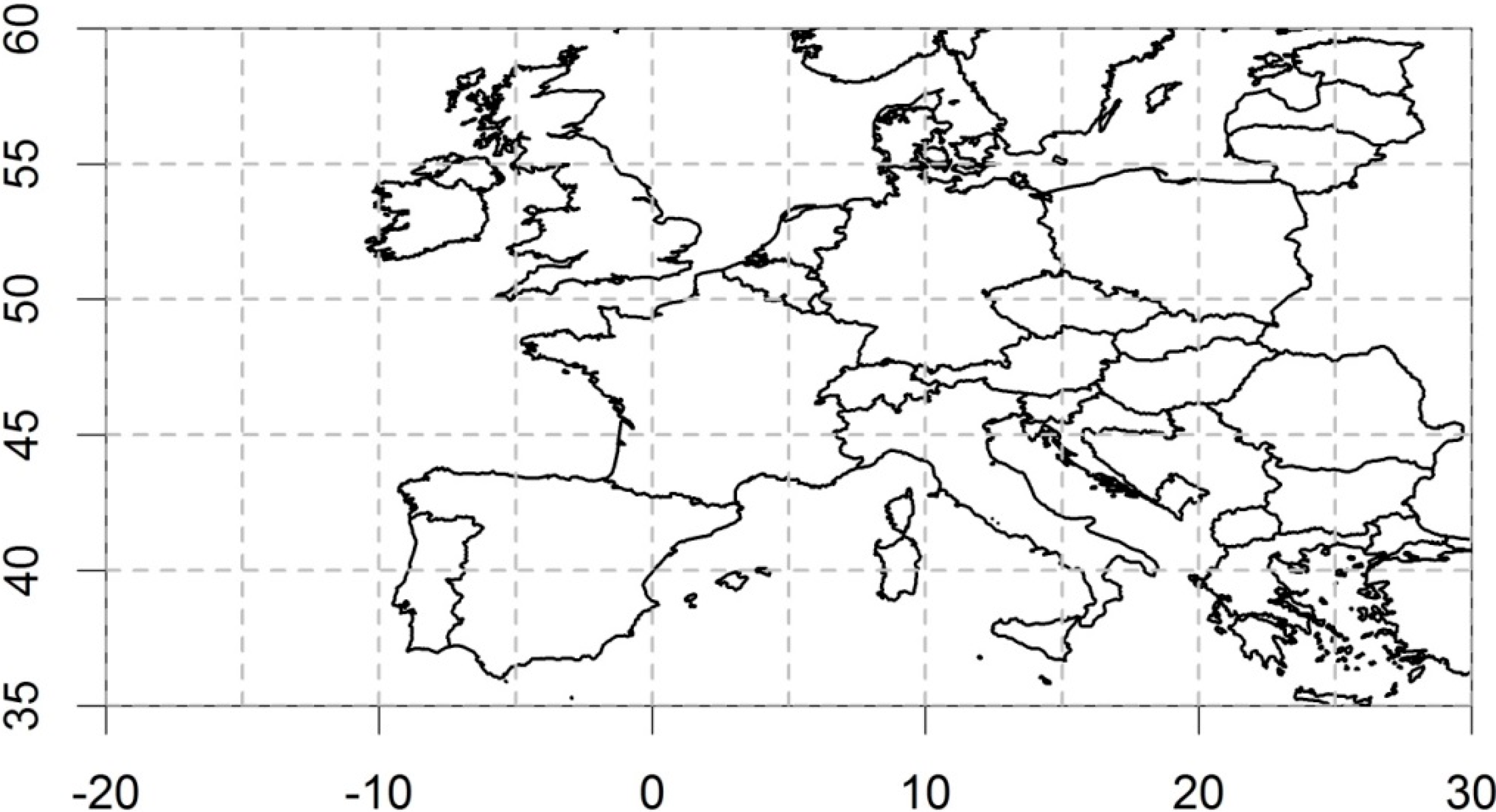
21]. In the combination of the original meteorological station data series, the calculation of anomalies from the temperature data is necessary to account for stations being located at different elevations within each grid box. For this study, the grid boxes covering Central Europe (excluding Scandinavia) were extracted, covering latitudes 35°N to 60°N and longitudes 20°W to 30°E (the full extent of the map in
Figure 1). Any grid box time-series with fewer than 500 values were excluded from the analysis. After the MSE analysis for each grid box time-series, the entropy values for each scale factor were averaged and their standard error calculated across all grid boxes.
Figure 1.
Area for which CRUTEM4v surface temperature anomaly data were extracted and analysed for each 5° × 5° grid box using multi-scale entropy (MSE). Country outlines data source: GISCO—Eurostat (European Commission). Administrative boundaries: EuroGeographics©, UN-FAO, Turkstat.
Figure 1.
Area for which CRUTEM4v surface temperature anomaly data were extracted and analysed for each 5° × 5° grid box using multi-scale entropy (MSE). Country outlines data source: GISCO—Eurostat (European Commission). Administrative boundaries: EuroGeographics©, UN-FAO, Turkstat.
The CRUTEM4v variance-adjusted temperature anomaly data for Central Europe are split into two time periods of 1850–1960 and 1961–2014. This division was based on two considerations: First, 1961–1990 is the reference period used to combine the station temperature anomalies for each grid box. Second, starting in the 1960s, industrialization intensified very quickly, leading to rapidly changing global anthropogenic greenhouse gas emissions from fossil fuel burning, cement production and tropical deforestation. This step change is evident from the global greenhouse gas emission record [
22].
3. Results
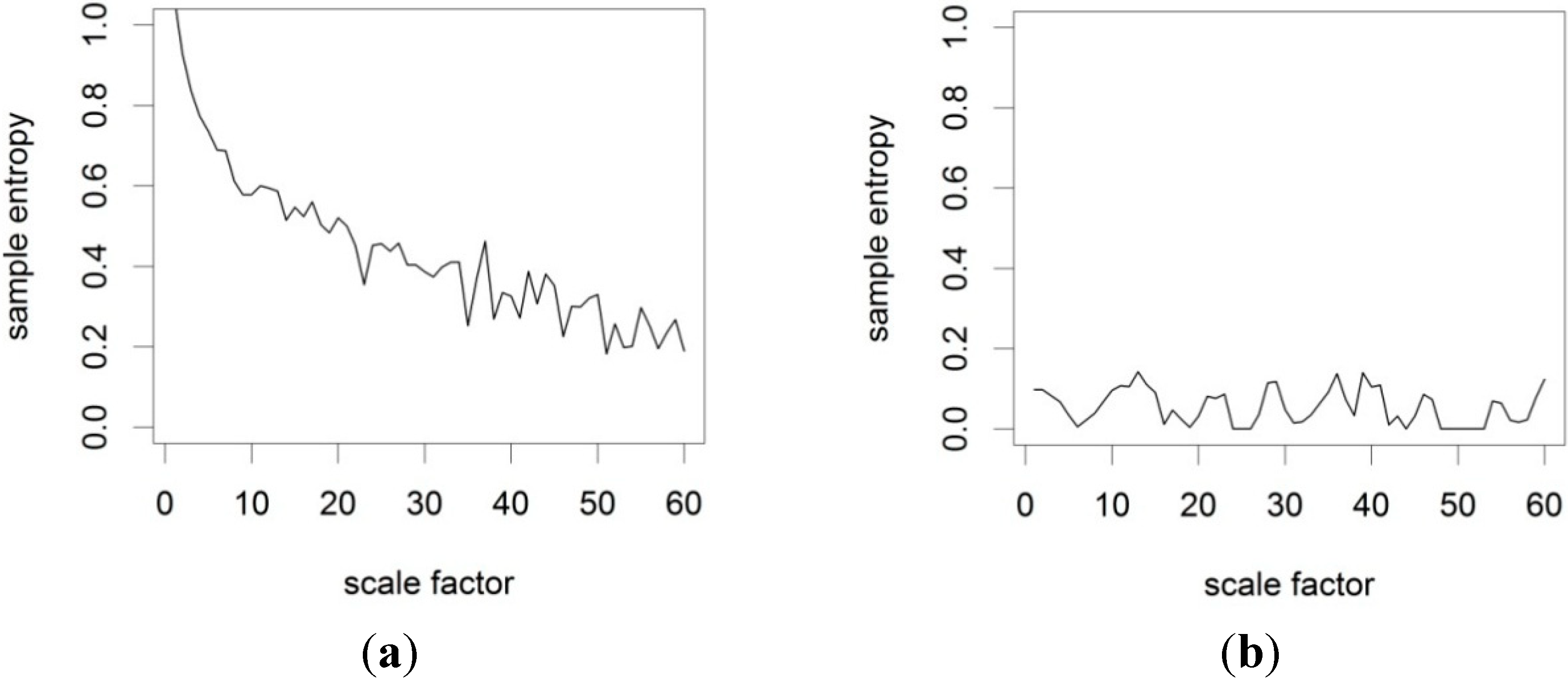
In order to test the MSE analysis code on time-series data with known statistical properties, two artificial time-series of length
N = 2000 were created. These datasets were created to test the algorithm on one random and one deterministic time-series. Dataset 1 is a uniform white noise time-series with a data range from 0 to 100 and Dataset 2 is a sine function for x value increments of 0.25.
Figure 2 shows the results for both artificial datasets. The white noise data show high entropy for low τ which decreases non-linearly for large τ. This behaviour was previously reported by Costa
et al. [
11] and Li and Zhang [
9]. For the sine function data the entropy is generally very low in comparison to the white noise data, indicating a high degree of order in the data. This preliminary analysis shows that the MSE code produces consistent results with previous implementations.
Figure 2.
Multi-scale sample entropy of: (a) an artificial uniform white noise time-series; and (b) a sine function.
Figure 2.
Multi-scale sample entropy of: (a) an artificial uniform white noise time-series; and (b) a sine function.
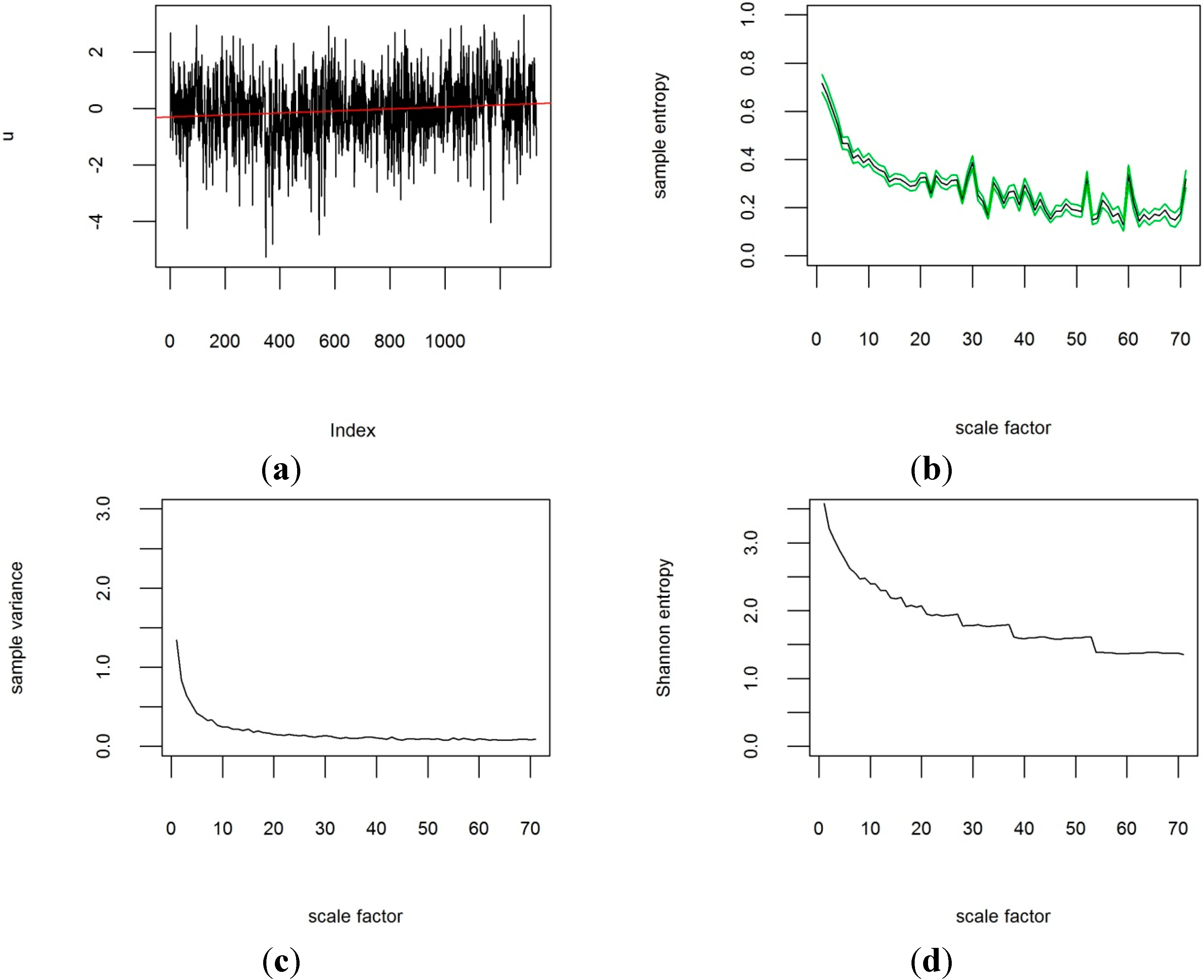
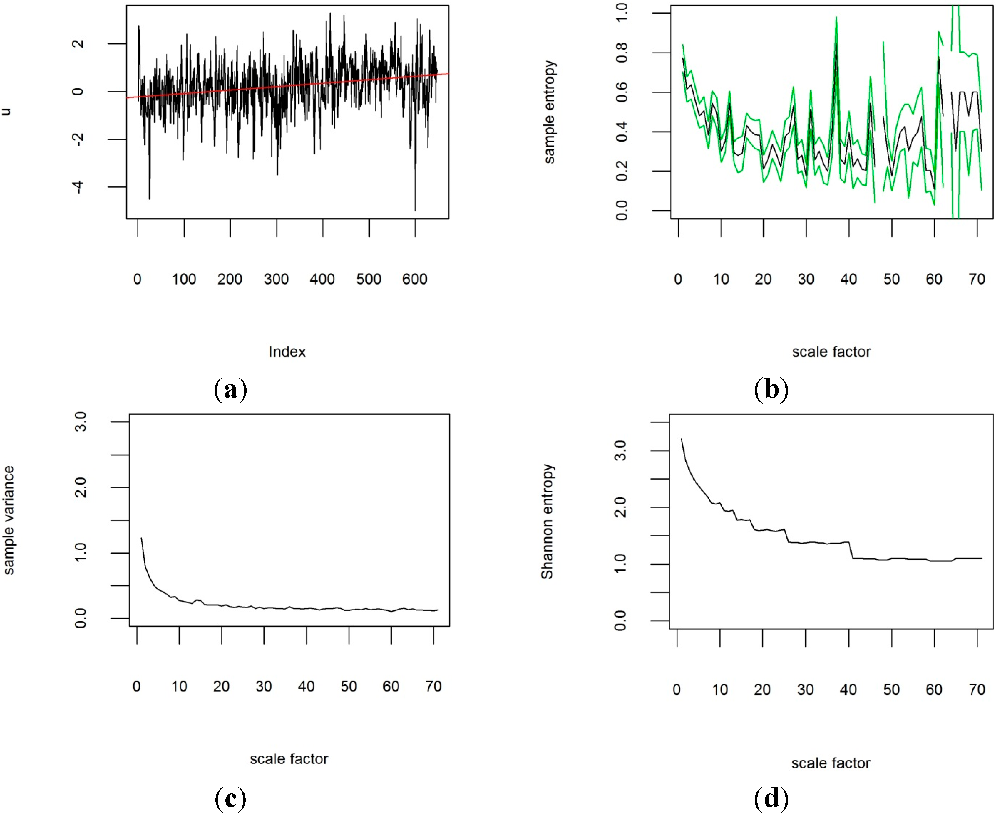
For the analysis of the CRUTEM4v data, plots of the sample entropy were created for each grid cell at all different temporal scales. As an example,
Figure 3 shows the results of the MSE analysis of the time period from 1851 to 1960 for the grid box row 8, column 35, covering the Republic of Ireland centred on 52.5° latitude and −7.5° longitude, along with the original time-series data, the variance and Shannon entropy for the coarse-grained time-series at each temporal scale factor. The same results are shown in
Figure 4 for the last 50 years from 1961 to 2014 for comparison. These two figures show that the MSE contains additional information to the variance and information theoretic entropy after Shannon: The variance in
Figure 3c and
Figure 4c does not show any changes in the behaviour of the temperature time-series on first inspection. Neither does the Shannon entropy at any timescales in
Figure 3d and
Figure 4d, apart from a slight shift to lower values. However, when comparing the sample entropy of the temperature anomalies from 1850 to 1960 (
Figure 3b) to 1961 to 2014 (
Figure 4b), the temporal scaling appears to have changed, with peaks appearing in
Figure 4b that are not discernible in
Figure 3b. For scale factors above approximately 8–12 months, the sample entropy has increased in the more recent past for that grid box.
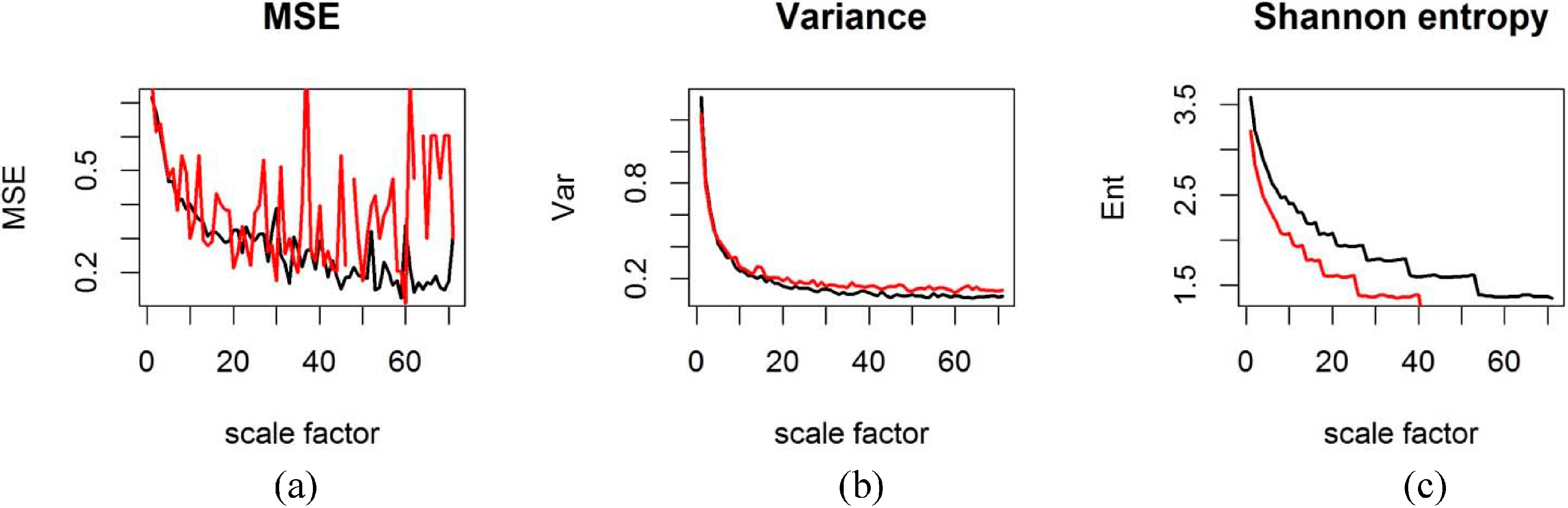
Figure 5 compares the sample entropy for the two time-periods and contrasts this plot with the variances and Shannon entropy for both time periods, calculated with different degrees of coarse-graining. A change in the variance of grid-box temperature anomalies at different temporal scales is observed in
Figure 5b, but the variance does not show any spikes like the sample entropy in
Figure 5a. Only the sample entropy allows the identification of specific temporal scales of variability in the time-series data at which the degree of order in the data has increased or decreased. MSE is independent of the variance if normalized correctly, which means that the changes in scaling behaviour of temperature anomalies affect both the variance and complexity of the system (quantified by MSE). MSE analysis can thus detect properties of the time-series that are undetected by traditional statistical methods. The uncertainty in the multi-scale sample entropy estimates is quantified for each grid cell based on the 95% confidence intervals derived under the assumption of a t-distribution following the method by Richman and Moorman [
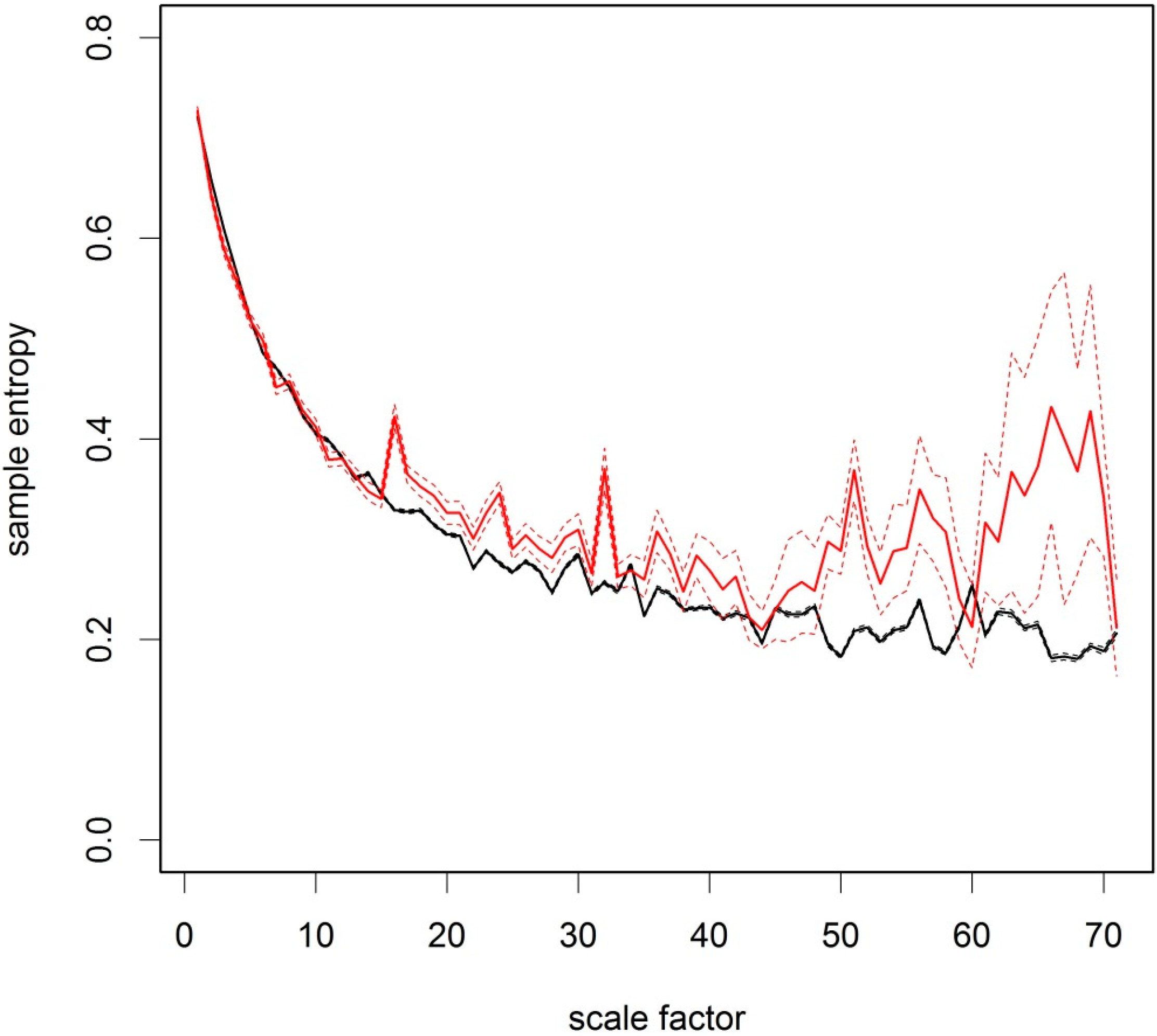
8]. In the next step of the analysis, the sample entropy is averaged over all grid boxes and their 95% confidence intervals are aggregated by adding up the squared standard errors and taking the square root of the sum, adjusting for uneven numbers of samples. The aggregated results for the whole study region in
Figure 6 shows that the temperature anomalies from 1850 to 1960 over Central Europe generally follow the shape expected from a white noise process (
Figure 2a). In contrast, the more recent temperature anomaly data from 1961–2014 show a different scaling behaviour (
Figure 6). The sample entropy for 1961–2014 for scale factors greater than 12 months has increased in comparison with the period before 1960. The 95% confidence intervals for the time period before and after 1960 do not overlap at many scale factors between 12 and 70 months, indicating statistically significant differences.
Figure 3.
Time-series from 1851–1960 of CRUTEM4v variance-adjusted surface temperature anomaly data for grid box [8|35] centred on 52.5° latitude and −7.5° longitude, with m = 3 and r = 0.3. Scale factor is shown in months. (a) original time-series; (b) multi-scale sample entropy for the grid box (95% confidence intervals in green) against scale factor; (c) sample variance for different scale factors; (d) Shannon information theoretic entropy for different scale factors.
Figure 4.
Time-series from 1961–2014 of CRUTEM4v variance-adjusted surface temperature anomaly data for grid box [8|35] centred on 52.5° latitude and −7.5° longitude, with m = 3 and r = 0.3. Scale factor is shown in months. (a) original time-series; (b) multi-scale sample entropy for the grid box (95% confidence intervals in green) against scale factor; (c) sample variance for different scale factors; (d) Shannon information theoretic entropy for different scale factors. For the MSE in (b), missing data points represent scales at which no template matches were found.
Figure 5.
Sample entropy, variance and Shannon entropy for the time-series of CRUTEM4v variance-adjusted surface temperature anomaly data for grid box [8|35] with m = 3 and r = 0.3. Black = 1851–1960; Red = 1961–2014. (a) multi-scale sample entropy for the grid box against scale factor; (b) sample variance for different scale factors; (c) Shannon information theoretic entropy for different scale factors (months).
Figure 6.
Multi-scale sample entropy of the CRUTEM4v variance-adjusted surface temperature anomaly data over Central Europe for m = 3 and r = 0.3. Scale factor is shown in months. Black = 1850 to 1960. Red = 1961 to 2014. Bold lines show the mean of all grid boxes and thin lines show the upper and lower bounds of the 95% confidence interval based on the t-distribution.
The MSE results suggest that the complexity (
sensu Costa
et al. [
11]) of the temperature anomaly time-series data at time-scales over 12 months is now greater than before 1960. Such a change in sample entropy can be caused by the behaviour of systems of greater complexity which tend to generate more “random” (less regular) responses than simpler systems, producing higher sample entropy. Simpler systems that are governed by a small number of deterministic processes tend to show lower sample entropy values. If more and more such deterministic processes are added into the system, its overall behaviour can appear more random. The climate system is a prime example for such complexity.
In conclusion, the results in
Figure 6 are consistent with H
1 that regional temperature anomalies in Europe show particular time-scales with higher sample entropy than expected under the assumption of white noise. This only holds for the more recent data from 1961 to 2014, where signals in the time-series are apparent at specific time-scales where spikes in sample entropy are detected.
The results support hypothesis H
2 that the sample entropy of European temperature anomalies shows significant differences at particular time-scales when comparing 1851–1960 with 1961–2014. We infer that the temporal scaling properties of the temperature data have changed at the specific temporal scales of observation shown by significant deviations in
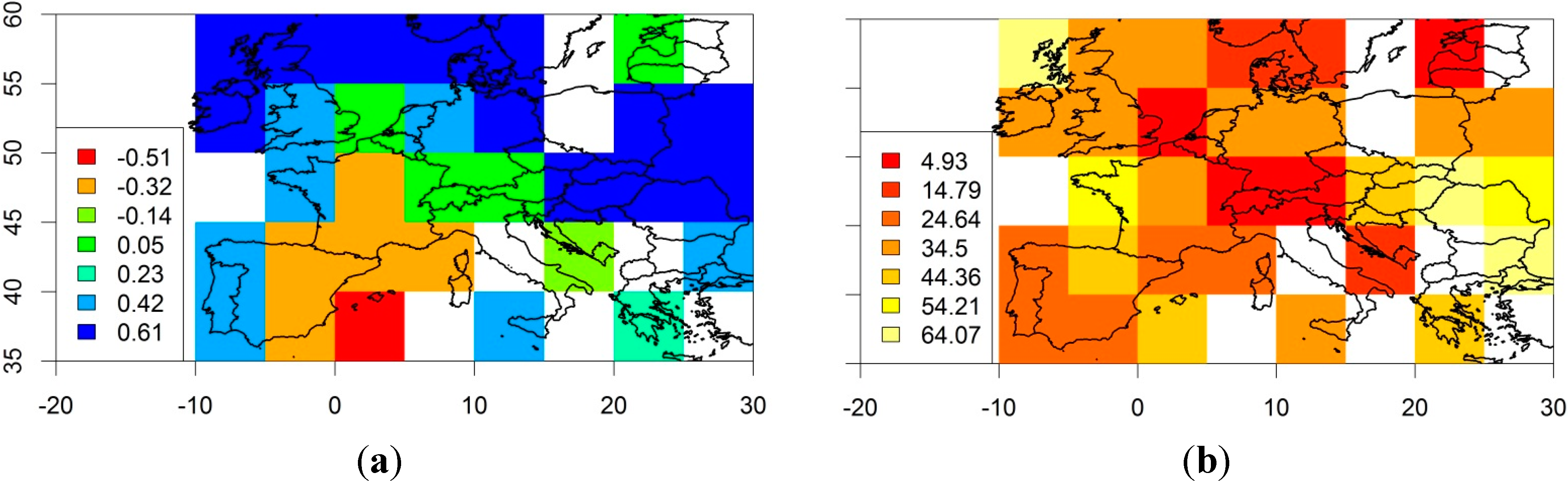
Figure 6.The regional scale analysis in
Figure 6 is based on the assumption that regional aggregation of the estimation of the sample entropy at different time-scales is more robust than a detailed grid-box level analysis because it is based on a larger number of meteorological stations. However, the visualization of the spatial patterns of the changes in temporal scaling behaviour may lead to further insights. The challenge is to visualize a complex dataset as a 2D map. For each grid box the MSE analysis results in a multi-scale plot like the one shown in
Figure 3. Consideration needs to be given to the metrics of interest before mapping the results from this analysis. We can examine the difference between the sample entropy at a particular timescale between 1850–1960 and 1961–2014, for example. The selection of a timescale at which to visualize the differences is not straightforward. Here, the timescale with the largest absolute difference in sample entropy was chosen. In the map of Central Europe in
Figure 7a, the colour scale represents the magnitude of the largest change in sample entropy (increase or decrease at any scale factor). It shows that Southern France, Eastern Spain and Corsica have experienced a decrease in sample entropy between 1850–1960 and 1961–2014. Portugal, the Bretagne, Great Britain, Ireland, Northern Germany and Eastern Europe showed a significant increase in sample entropy at particular timescales. At which timescales do these changes in sample entropy occur?
Figure 7b shows a map where the colours represent the temporal scale factor at which the largest absolute difference in sample entropy occurs. In
Figure 7b it is apparent that there is no consistent pattern of the scale factors at which the largest change in sample entropy occurred, but many areas show scale factors between 20 and 40.
Figure 7.
Map of Central Europe indicating the grid boxes where the CRUTEM4v variance-adjusted surface temperature anomaly data show a statistically significant (p < 0.05) change in multi-scale sample entropy. Non-significant values are set to zero. (a) Magnitude of the largest change in sample entropy detected across all scale factors. Negative values show a decrease from 1850–1960 to 1961–2014. (b) Corresponding scale factor at which the largest absolute difference in sample entropy occurred (months).
4. Discussion
This study has applied MSE analysis to a climatic dataset for the first time, in order to evaluate whether this technique can provide useful information on the time-series analysis of climate data. This was achieved by carrying out an MSE analysis of the CRUTEM4v variance adjusted air temperature anomaly data over Central Europe.
MSE analysis was able to detect specific changes in the complexity of the time-series at specific time-scales of aggregation (>12 months), which went undetected by a multi-scale variance analysis and by the Shannon entropy at multiple scales. This finding shows that MSE analysis provides additional information on the timescales at which the data show a change in their temporal behaviour.
The results also demonstrate that in Central Europe the complexity of the regional temperature data, which are an expression of the processes in the climate system, has changed its temporal scaling behaviour since the 1960s (
Figure 6). This is consistent at a regional scale with findings by Rossi
et al. [
7] who used wavelet analysis to show that frequency changes in several climate indices demonstrated a major and global shift in the climate system.
The results show that patterns of Central European air temperatures have recently become less regular on time-scales longer than 12 months compared to the period before 1960. This increasing complexity in the time-series is only noticeable on time-scales longer than 12 months, which indicates that knowledge of the scales of variability is necessary to detect these patterns in temperature data. The results found here are consistent with reports of frequent heat waves, cold spells, droughts and floods experienced by many regions in Europe over recent decades. An exceptionally high number of extreme heat waves have been observed around the world in the last ten years [
23], for example the European heat wave of 2003 [
24]. A review of extreme weather patterns at temporal scales from days to months [
1] concludes that in recent years an “exceptionally large number of record-breaking and destructive heatwaves” were observed in many parts of the world. This increase in the probability of such extreme events is most likely linked to global warming [
1].
Similar changes can be observed in the water cycle in Europe. Many meteorological stations in Europe have shown changes in the duration of dry and wet spells between 1950 and 2009 [
25], with climate model predictions suggesting that Northern Europe is likely to experience wetter conditions and Southern Europe drier conditions under climatic change [
26].
It has been suggested that the temporal scales of extreme weather events might increase in duration. Possible causes of the temporal scaling properties of northern hemisphere weather patterns are still subject to intense scientific debate. One explanatory line of thought is asking whether longer durations of extreme weather patterns in Europe could be influenced by slowing circumpolar winds in the arctic due to rapid surface warming and diminishing sea ice extent. A recurrent global teleconnection pattern in the summertime mid-latitude circulation of the northern hemisphere, accompanied by rainfall and air temperature anomalies in Western Europe, was discovered in a 56 year NCEP-NCAR reanalysis dataset by Ding and Wang [
27]. Heat waves might in future last for periods of months rather than days or weeks. A slower progression of upper-level atmospheric Rossby waves in the northern hemisphere is a possible explanation of this phenomenon. Slower Rossby waves would cause more persistent associated weather patterns in mid-latitudes, which “may lead to an increased probability of extreme weather events that result from prolonged conditions, such as drought, flooding, cold spells, and heat waves” [
28].
5. Conclusions
For the first time, multi-scale sample entropy analysis (MSE) has been applied to central European air temperature anomaly data from 1850 to 2014. MSE provides additional information on changes in the temporal scaling behaviour of central European climate time-series, when compared to multi-scale variance and the Shannon entropy.
The gridded European variance-adjusted air temperature anomaly data reveal that in the period from 1961–2014, the sample entropy is markedly increased at time-scales from 12 to 70 months compared to 1851–1960. This increase in sample entropy at specific timescales shows at which temporal scales the temperature data have increased in complexity.
The visualization of the largest absolute change in sample entropy and the timescales at which this was observed proved effective at discerning spatial patterns of temporal changes in complexity. The analysis also shows that such changes are only detected at specific identifiable timescales.
This research demonstrates that MSE analysis provides a statistical tool that can detect changes in climatological time-series data. Future work should examine the relation of MSE to climate oscillation and teleconnection patterns (e.g., NAO, El Niño) and application to other climate time-series data.

 ,
, 


