Abstract
This paper aims to build a Self-supervised Fault Detection Model for UAVs combined with an Auto-Encoder. With the development of data science, it is imperative to detect UAV faults and improve their safety. Many factors affect the fault of a UAV, such as the voltage of the generator, angle of attack, and position of the rudder surface. A UAV is a typical complex system, and its flight data are typical high-dimensional large sample data sets. In practical applications such as UAV fault detection, the fault data only appear in a small part of the data sets. In this study, representation learning is used to extract the normal features of the flight data and reduce the dimensions of the data. The normal data are used for the training of the Auto-Encoder, and the reconstruction loss is used as the criterion for fault detection. An Improved Auto-Encoder suitable for UAV Flight Data Sets is proposed in this paper. In the Auto-Encoder, we use wavelet analysis to extract the low-frequency signals with different frequencies from the flight data. The Auto-Encoder is used for the feature extraction and reconstruction of the low-frequency signals with different frequencies. To improve the effectiveness of the fault localization at inference, we develop a new fault factor location model, which is based on the reconstruction loss of the Auto-Encoder and edge detection operator. The UAV Flight Data Sets are used for hard-landing detection, and an average accuracy of 91.01% is obtained. Compared with other models, the results suggest that the developed Self-supervised Fault Detection Model for UAVs has better accuracy. Concluding this study, an explanation is provided concerning the proposed model’s good results.
1. Introduction
In the 21st century, with the development of information technology, UAVs have become a popular industry in this new round of global technological and industrial revolution. With the extensive use of UAVs, the importance of UAV safety has been paid increasing attention. A UAV is a complex system with multidisciplinary integration, high integration, high intelligence, and low-redundancy design [1]. Therefore, improving the safety of UAVs is an important goal in the industry. Due to the presence of a large number of factors, such as the electrical system, engine, and flight control, UAV faults are difficult to detect in business scenarios [2,3]. In UAV Flight Data Sets, most of the data are normal data, and the unbalanced data cause difficulties in detecting faults [4]. The traditional fault detection method is to monitor a certain factor; when the safety range is exceeded, a fault occurs. However, UAVs are complex systems, and a fault is caused by multiple factors [5]. At present, self-supervised fault detection based on Auto-Encoders has become the main research direction [6]. Representation learning is used to extract features. With the help of an Auto-Encoder, features from the flight data are extracted to build a Self-supervised Fault Detection Model for UAVs.
The multiple features in the data contained in the UAV Flight Data Sets included navigation control, the electrical system, the engine, steering gear, flight control, flight dynamics, and the responder [1]. An Auto-Encoder was used to extract the features and reduce the dimensions of the data. In the Auto-Encoder, a high-frequency signal in the data will affect the feature extraction of the model. We used wavelet analysis to extract the small-amplitude high-frequency signal in the data, which is similar to a random Gaussian signal. There was no need to pay attention to the random Gaussian signals with fewer features, and the Auto-Encoder was used for the feature extraction and reconstruction of the low-frequency signals with different frequencies. The normal data were used for training. The reconstruction loss of the low-frequency signals with different frequencies was weighted and averaged. The reconstruction loss was used as the criterion for fault detection. This method overcomes the problem of unbalanced data and low signal-to-noise ratio in data sets. To improve the effectiveness of the fault localization, an edge detection operator was used to calculate the reconstruction loss of the features in the UAV Flight Data Sets. The features with large reconstruction losses were considered fault features. The proposed method was verified in the UAV Flight Data Sets, and the results suggest the proposed prediction model has better performance. Compared with other studies, this study provides the following innovations:
- Aiming at the problem of UAV fault detection, we developed a new Self-supervised Fault Detection Model for UAVs based on an Auto-Encoder and wavelet analysis;
- As an efficient representation learning model, the Auto-Encoder overcomes the problem of insufficient fault data in the data sets and reduces the dimensions of the data. Wavelet analysis was used to process the data, which overcomes the problem of low signal-to-noise ratio in data sets;
- The loss of the Auto-Encoder and the edge detection operator were used to locate fault factors for further fault detection. Faults caused by multiple factors were detected.
The rest of this paper is organized as follows. In Section 2, related works are introduced, including the data feature extraction and model improvement. Section 3 shows our overall framework and proposed method. In Section 4, the effectiveness of the proposed Self-supervised Fault Detection Model for UAVs is evaluated using the UAV Flight Data Sets. The proposed model was compared with other models in the literature. In Section 5, the study is concluded.
2. Related Work
With the development of deep learning and the importance of data science, data-driven fault detection models have been developed. Data-driven fault detection models mainly include data feature extraction and model improvement [7].
2.1. Data Feature Extraction
Data obtained from sensors usually contain a lot of noise, and the features of the signals are often included in different frequencies. Therefore, data preprocessing is very important. Luo et al. [8] used integrated empirical mode decomposition to construct a data feature set, including energy features, frequency features, and singular value features. Li et al. [9] used wavelet transform to extract statistical variables from signal data, and the data features were used for the fault analysis of gear machines. Cheng et al. [10] used integrated empirical mode decomposition to obtain the natural mode function, and the entropy characteristics of the data were used for the fault analysis of the planetary gears. Meng Z. et al. [11] developed a balanced binary algorithm. For signal enhancement, the texture features of the signals are extracted by the improved algorithm. Gao K. et al. [12] developed a fault detection model combining adaptive stochastic resonance (ASR) and ensemble empirical mode decomposition (EEMD). The proposed model was used to solve the problem of weak early fault signals of rotating machinery. Weak fault signals are difficult to fault diagnose. Shao Y. et al. [13] developed a new filtering model based on extended bidimensional empirical wavelet transform. Irregularities in the manufacturing process of the workpiece were detected by the proposed model. In order to address the problem of the spectrum segmentation of the EWT method, Liu Q. et al. [14] aimed to improve the EWT model. The developed model efficiently extracted the fault features of bearings. The fault data of wind turbine gearbox bearings and locomotive bearings verified the efficiency of the developed model. Zhang Y. et al. [15] developed a novel fault detection model based on discrete state space construction and transformation. In the developed fault detection model, the high-dimensional features of raw signals were extracted, and the high-dimensional features were discretized into labels, which represent potential states of the operating conditions. The proposed model was verified in the fault detection of a compound compressor. Li Y. et al. [16] developed a new model that comprehensively considered local and global features. The inherent features of the signals were extracted by the global–local preserving projection (GLPP) model. The features of the signals were extracted by the global–local marginal discriminant preserving projection (GLMDPP) model. Long Z. et al. [17] developed a new fault diagnosis method that established the mapping relationship between intuitive image features and actual faults. The mapping is based on scale-invariant feature transform and symmetrized dot patterns. The dictionary templates are established by the normal and fault signals of motors. The matching point with the dictionary templates is counted for fault analysis. Zhang Y. et al. [18] presented a new fault detection model based on an Auto-Encoder. This study proposed a gated recurrent unit (GRU) and a deep Auto-Encoder. The spatial–temporal features of the data are fused by the proposed deep Auto-Encoder. The symmetric framework of the presented model extracts the spatial–temporal features of the data. The temporal feature extraction capability of the GRU and the spatial feature extraction capability of the Auto-Encoder were combined in this study. To reduce the influence of these factors on the feature extraction, Su N. et al. [19] presented a novel model for fault diagnosis and feature extraction. The presented model is based on high-value dimensionless features and is used for bearings in the petrochemical industry. Lei D. et al. [20] proposed an understandably weak fault information method that combines deep neural network inversion estimation. The weak fault information is intuitively identified from the original signals by the proposed model. In the original input feature space, the most sensitive input pattern is extracted by the proposed model to maximize the neuron’s activation value of the network output layer.
2.2. Model Improvement
In addition, the improvement of the model parameters and structure can also improve the detection accuracy and efficiency, and many models combined with deep learning have been developed in recent years. Fu Y. et al. [21] presented the VGG16 fault analysis model. The presented model is based on a multichannel decision level fusion algorithm, with symmetrical point pattern (SDP) analysis. Deng W. et al. [22] developed a new fault analysis model, which is used for the rotating machine. The kernel parameters and penalty parameters of the support vector machine (SVM) are optimized by the improved particle swarm optimization (PSO) model. Jahromi A. T. et al. [23] developed a new fault analysis model, the sequential fuzzy clustering dynamic fuzzy neural network (SFCDFNN). The proposed model is used for the fault monitoring of high-speed cutting processes. Amozegar M. et al. [24] developed a new fault detection model, which was verified by the fault detection and isolation (FDI) of gas turbine engines. The presented model combines a fusion neural network under a multiple-model architecture and is used for the FDI of the gas path. Three individual dynamic neural network architectures were constructed to identify the dynamics of the gas turbine engine and to achieve fault monitoring. Wang K. et al. [25] developed a multichannel long short-term memory network (LSTM) combining a sliding window. The proposed model explores the spatial and temporal relationships of the data, and the residuals of sensor measurements between the observed and predicted values are captured. Liu X. et al. [26] proposed an ensemble and shared selective adversarial network (ES-SAN). In machinery fault analysis, the presented model is used to address the problem of partial domain adaptation (DA). Sun R. et al. [27] proposed a new game theory-enhanced DA network (GT-DAN). GT-DAN combines different metrics, including the maximum mean discrepancy, Wasserstein distance, and Jensen–Shannon divergence. The distribution discrepancies between the target domain and the source domain are described by three attention matrices, which are constructed by the model. In machinery fault analysis, this study was verified by solving the problem of domain adaptation (DA). Han T. et al. [28] presented a new fault detection framework, which combines the spatial–temporal pattern network (STPN) method and convolutional neural networks (CNNs). This study built a hybrid ST-CNN scheme for machine fault diagnosis. Yang L. et al. [1] proposed a fault detection model based on complete-information-based principal component analysis (CIP-CA) and a back propagation neural network (BPNN). The proposed model was verified using real UAV flight data sets. Su Z. et al. [29] developed a multifault detection model for rotating machinery. The proposed model combines a least square support vector machine (LS-SVM) and orthogonal supervised linear local tangent space alignment (OSLLTSA). To solve the problem of the hypergraph being unable to accurately portray the relationships among the high-dimensional data, Yuan J. et al. [30] proposed a new dimensionality reduction model called semi-supervised multigraph joint embedding (SMGJE). Simple graphs and hypergraphs with the same sample points are constructed by SMGJE, and the structure of the high-dimensional data are characterized by SMGJE in a multigraph joint embedding. This study was verified by the fault detection of rotors. Zhou S. et al. [31] presented a new model based on a combination of weighted permutation entropy (WPE), ensemble empirical mode decomposition (EEMD), and an improved support vector machine (SVM) ensemble classifier. The efficiency of the presented model was proved by rolling bearing fault analysis. In order to evaluate the landing quality of UAVs, Zhou S. et al. [32] aimed to use the VIKOR algorithm based on flight parameters. The model is used to determine the parameter interval of landing quality classification. Zhang M. et al. [33] proposed a wavelet singular spectral entropy model that combines the singular value, wavelet analysis, and information entropy. The distribution complexity of the spatial modalities is described by the proposed model, and the proposed model accurately distinguishes the boundary between the unstable and stable states from the view of a dynamic system. Du X. et al. [34] proposed a convolutional neural network (CNN) model whose basic unit is an initial block. The initial block is composed of the convolution of different sizes in parallel. Redundant signals between the multiple sensors are fully extracted by the convolution of the proposed model. The proposed model achieves accurate information extraction and is used for the fault detection of aeroengine sensors. In order to extract the features, Swinney C. J. et al. [35] input a spectrogram, raw IQ constellation, and histogram as graphical images to a deep convolution neural network (CNN) model, which is called ResNet50. The proposed model is pre-trained on ImageNet, and transfer learning is used to reduce the demand for large signal data sets.
In addition, some scholars have used model-based methods for the fault detection and identification of UAVs. Asadi D. et al. [36] presented a new two-stage structure that generates a residual signal using parity space. The residual signal is detected by the exponential forgetting factor recursive least square method. Asadi D. et al. [37] presented a new fault detection algorithm using the controller outputs and the filtered angular rates. Hu C. et al. [38] developed a fault detection model for a hypersonic flight vehicle. The model is based on a sliding mode observer. A simulation experiment achieved good results. Wen Y. et al. [39] presented a fault detection scheme. The filter is used as a residual generator. The solvable condition of the fault detection model is established by the residual.
3. UAV Flight Data Sets and Proposed Model
Section 3 introduces the UAV Flight Data Sets and the overall framework of the Self-supervised Fault Detection Model for UAVs. The methodological framework of this study is shown in Figure 1.
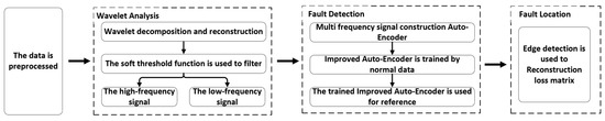
Figure 1.
The methodological framework of this study.
In Figure 1, the overall framework is divided into four parts. First, the data are preprocessed, including data cleaning and normalization. Second, wavelet analysis is used to process the data. Then the Auto-Encoder is used to extract and reconstruct the features of the flight data. Finally, we use the loss of the Auto-Encoder and the edge detection operator to locate fault factors for further fault detection.
3.1. Data Overview and Data Processing
The UAV Flight Data Sets are real data collected by long-term maintenance and repair work during the use of a certain UAV. The flight information of 28 sorties of a certain UAV was recorded by the UAV Flight Data Sets. The UAV Flight Data Sets include navigation control data sets, electrical system data sets, engine data sets, steering gear data sets, flight control data sets, flight dynamics data sets, and responder data sets. The navigation control data sets contain more than 100 factors concerning navigation control. The electrical system data sets record the status of the electrical system, including 19 factors. The engine data sets record the status of the engine, including more than 60 factors. The steering gear data sets record the status of the steering gear, including more than 100 factors. The flight control data sets record the information of the UAV flight control, including 26 factors. The flight dynamics information of UAVs is recorded in the flight dynamics data sets, which contain more than 100 factors. The signals of the responder are recorded in the responder data sets, which contain 23 factors. The UAV Flight Data Sets contain approximately 53.5 million data records, and more than 500 factors are contained in each data set, as shown in Table 1.

Table 1.
More than 500 factors are contained in each data set.
Data preprocessing is an important prerequisite step in the process of data analysis. There are always missing data and invalid data in the original data set. We analyzed the data sets and eliminated the invalid data and unreasonable data. If some data were null, we used the average of the nearby values. For the data analysis, the data were normalized by the min–max method, as follows:
where is the normalized data, is the original data in the data sets, is a function that returns the minimum value of the input value, and is a function that returns the maximum value of the input value. It should be noted that different factors are collected by different sensors. However, different sensors have different data collection periods. For the flight data, the data are split from the time dimension. In order to align the data period, some data are interpolated as follows:
where is the interpolated data, , , , and are the contiguous data of the interpolated data. The interpolation of the data is shown in Figure 2.
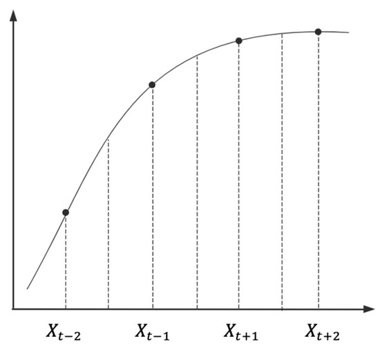
Figure 2.
The interpolation of the data.
Some data (data with a too-long data period) are interpolated to align the data period. Some data (data with a too-short data period) used averages to align the data period. For data feature extraction, all factors should obtain the same data period. Interpolated data or average data are more reasonable.
After the data preprocessing, the data are composed of multiple two-dimensional matrices. Each matrix denotes the flight data of a UAV. Each matrix is as follows:
where is the flight data of a UAV, the Y axis denotes the factors that affect the fault of the UAV, and the X axis denotes the time. For example, denotes the value of factor at time . Obviously, the flight data are composed of multiple time series. The multiple time series are as follows:
where are time series to be filtered.
3.2. Improved Auto-Encoder Based on Wavelet Analysis
In data science, representation learning is used to process the original data. Representation learning is used to extract the features of the original data. Flight data are typical high-dimensional large sample data sets, which are suitable for using representation learning to extract features and reduce data dimensions. An Auto-Encoder is a common representation learning model.
In UAV fault detection, the fault data only appear in a small part of the data sets. In the supervised learning model, the ability to extract fault features will be affected by unbalanced data. The unbalanced data cause difficulties in detecting faults. The self-supervised learning model overcomes this problem and provides a new perspective for fault detection. In the fault detection model, the high-frequency signal in the data affects the extraction of data features by the Auto-Encoder. Wavelet analysis can effectively extract the high-frequency signal in the data and separate the signals with different frequencies. Therefore, we used wavelet analysis to decompose and reconstruct the signal. This paper proposes a new Self-supervised Fault Detection Model for UAVs based on an Auto-Encoder and wavelet analysis.
3.2.1. Auto-Encoder
An Auto-Encoder is a self-supervised learning model that has been widely used in fault detection. An Auto-Encoder includes an encoder to obtain the encoding from the input data and a decoder that can reconstruct the input data from the encoding [40]. After training, the encoding can be used as a feature of the input data for the downstream task. The downstream task includes classification and regression. The Auto-Encoder’s specific structure is shown in Figure 3.
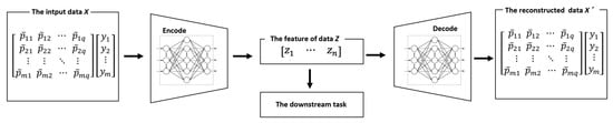
Figure 3.
Auto-Encoder’s specific structure.
Where is the input data, is the encoding generated by the encoder and represents the feature of the input data, and is the output data reconstructed by the decoder.
In self-supervised fault detection, only normal data are available as training data. The impact of the unbalanced data is avoided. Training on the normal data and fault data will produce a higher reconstruction loss in the Auto-Encoder, which is used for fault detection. When the reconstruction loss of the flight data exceeds the threshold value, the UAV faults in flight.
3.2.2. Wavelet Analysis
Wavelet analysis is used to effectively extract important information from data. Through the operations of stretching and translation, the signal can be analyzed in multiscale detail, and then the detailed features of the signal can be focused [41]. Decomposing the different frequency components of signals is one of the important functions of wavelet analysis.
Because of the filtering effect of the wavelet analysis, it is easier to analyze the features of the signals. Wavelet transform is the basis of wavelet analysis. The wavelet transform and inverse transform are as follows:
where is the inner product operation, is the wavelet basis function, is the stretching operation, is the translation operation, and is the admissible condition of the wavelet basis function. is as follows:
where is the Fourier transform of .
The Mallat algorithm is used for filtering, which is a discrete transformation [42]. The signal is decomposed by wavelet decomposition, which is divided into two parts: low-frequency coefficients and high-frequency coefficients. The wavelet decomposition of a time series is as follows:
where is the high-pass decomposition filter, is the low-pass decomposition filter, is the high-frequency coefficient, is the low-frequency coefficient, and is the discrete convolution operator. Both and depend on the wavelet basis function. The signal can be reconstructed by wavelet reconstruction. Wavelet reconstruction can calculate the low-frequency component from the low-frequency coefficients and calculate the high-frequency component from the high-frequency coefficients. The wavelet reconstruction of the signal is as follows:
where is the high-pass reconstruction filter, is the low-pass reconstruction filter, is the high-frequency signal, and is the low-frequency signal. Both and depend on the wavelet basis function. Using wavelet decomposition and reconstruction, the relationship between the low-frequency signal , the high-frequency signal , and the time series is as follows:
The process of wavelet decomposition and reconstruction is shown in Figure 4.
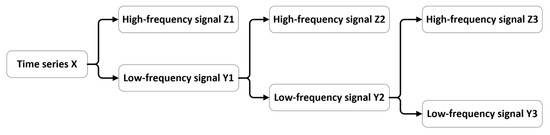
Figure 4.
The process of wavelet decomposition and reconstruction.
3.2.3. Improved Auto-Encoder
This paper improves on the Auto-Encoder by wavelet analysis. Flight data are composed of multiple time series. In a time series with a low signal-to-noise ratio, the high-frequency signal in the data affects the extraction of data features by the Auto-Encoder. Therefore, using wavelet analysis to filter noise is helpful for feature extraction.
The flight data are composed of multiple time series that need to be filtered. The high-frequency signal in the data sets is extracted by wavelet decomposition and reconstruction. The Db10 wavelet basis function and soft threshold function are used, and the number of wavelet layers is three [43]. The process of wavelet decomposition and reconstruction is shown in Figure 4. The time series is decomposed and reconstructed three times. After the three-layer wavelet decomposition and reconstruction, the high-frequency signals , , and are obtained. The high-frequency signals , , and are filtered using the soft threshold function. The soft threshold function is as follows:
where is the threshold, are the estimated wavelet coefficients, are the wavelet coefficients after decomposition, is taken between 0 and 1, and is the symbolic function. The filtered low-frequency signal and high-frequency signal are reconstructed.
After filtering, the high-frequency signals in the data are eliminated, and the low-frequency signals , , and are obtained. The data of each frequency contain different features. In order to better extract features, data with different frequencies will be used for reconstruction by the Auto-Encoder. The flight data are filtered to obtain the data of multiple frequencies. The data of multiple frequencies are as follows:
where ,, and are the data of multiple frequencies after filtering, which are composed of multiple time series.
The overall architecture of the improved Auto-Encoder is shown in Figure 5.

Figure 5.
The overall architecture of the improved Auto-Encoder.
The backbone of the improved Auto-Encoder is a CNN and self-attention module. Each self-attention module includes two submodules: a multihead attention module and a full connection network. Each multihead attention module has a residual connection. The self-attention module’s specific structure is shown in Figure 6.
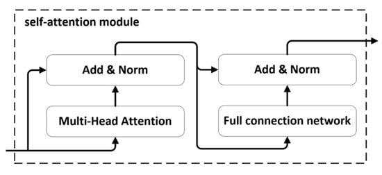
Figure 6.
Self-attention module’s specific structure.
The improved Auto-Encoder is a symmetrical neural network structure. The encoder and decoder are as follows:
where and denote the parameters of the encoder and decoder , respectively. For better representation learning, multiple prediction heads are associated with the Auto-Encoder for the reconstruction of data at different frequencies. The improved Auto-Encoder is as follows:
where , , and are the reconstruction of the different frequency data by the improved Auto-Encoder. In training, we use the norm-based MSE to measure the reconstruction quality, as follows:
where is the reconstruction loss, which is used as the criterion for fault detection at inference, and , , and are the individual loss weights. A flow chart of the proposed improved Auto-Encoder is shown in Figure 7.
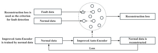
Figure 7.
The flow chart of the proposed improved Auto-Encoder.
The steps of the improved Auto-Encoder are as follows:
Step 1: The data are decomposed and reconstructed by wavelet, as follows:
where is the time series, which is input into the model, and and are the low-frequency signal and the high-frequency signal, respectively. only denotes normal data and is filtered as per Equation (11).
Step 2: The Auto-Encoder is used to train the low-frequency signal, as follows:
where is the Auto-Encoder, are the parameters of the Auto-Encoder, which is trained by normal data, and , , and are the reconstruction of the different frequency data by the Auto-Encoder.
Step 3: The trained Auto-Encoder is used for reference. The fault data will produce higher reconstruction loss. The reconstruction loss is used as the criterion for fault detection, as follows:
where is the test data at inference, is the reconstruction loss obtained by the trained Auto-Encoder, is the threshold value, and is the result of the fault detection. When the reconstruction loss of the flight data exceeds the threshold, the UAV faults in flight.
The pseudocode of the improved Auto-Encoder is shown in Algorithm 1.
| Algorithm 1: The improved Auto-Encoder |
| Input: The flight data , the test data at inference |
| Output: The result of fault detection |
| The flight data is decomposed and reconstructed by wavelet, as per Equation (12) |
| Train the Auto-Encoder using and the data of multiple frequencies after filtering , as per Equation (21) |
| for all |
| The trained Auto-Encoder is used for the reference, as per Equation (22) |
| The calculation of is based on the reconstruction loss, as per Equation (23) |
| end for |
| Return |
3.3. Fault Factor Location Based on the Edge Detection Operator
At the inference time, another problem that needs to be focused on has emerged, i.e., how to locate fault factors? In practical applications such as UAV fault detection, we need to know the factors and the time of the UAV fault. Traditional fault location based on random mask will increase the training time of a neural network [4]. To improve the effectiveness of fault localization at inference, we developed a new fault factor location method, which is based on the reconstruction loss of the Auto-Encoder and edge detection operator.
3.3.1. Edge Detection Operator
In digital image processing, edge detection has important applications. Pixels, the brightness of which changes significantly in digital images, are identified by edge detection. Significant changes in brightness usually represent important events and attributes. Edge detection is used to detect pixels whose values change significantly in digital images. The gradient of the pixels is used for edge detection. The Roberts operator is a commonly used edge detection operator [44]. The Roberts operator has two matrices, as follows:
The Roberts operator is as follows:
where is the horizontal filter value and is the vertical filter value. The horizontal filter value and the vertical filter value are as follows:
where is the digital image to be processed.
3.3.2. Fault Factor Location Based on Reconstruction Loss
The reconstructed data from the Auto-Encoder provide important information for fault factor detection. The reconstructed data are used to compare with the real data, and the reconstructed loss matrix is obtained. Different from the reconstruction loss, the reconstruction loss matrix records the average loss of each datum. The reconstruction loss matrix is as follows:
where is the reconstruction loss matrix. It should be noted that Equation (28) is different from Equation (19). denotes the absolute value of each element in the matrix and returns a matrix. The reconstruction loss matrix records the reconstruction loss of each datum. Data with a large reconstruction loss can be obtained from the reconstruction loss matrix. For example, when is a large value, factor is abnormal at time , which may be the cause of the UAV fault.
Traditional methods usually use the threshold value to calculate the data of the reconstruction loss matrix. However, the threshold value is usually calculated manually. The value of the threshold will affect the accuracy of the fault factor location. To improve the efficiency of the fault localization at inference, we propose a novel fault factor location method that is based on the Roberts operator. The Roberts operator calculates the gradient for the edge detection. For the reconstruction loss matrix, we needed to pay attention to the data with large gradient changes, because the change denotes that there is a large value in the matrix. The Roberts operator is used to locate the fault factor, as follows:
where denotes the results of the Roberts operator. In the results, the part with a large gradient change is considered as the factor causing the fault. The threshold value of the gradient is set to determine the factors in which the gradient is greater than the threshold value. The edge detection operator can realize the fault factor location of multiple factors.
4. Experiment and Discussion
In order to verify the efficiency of the developed Self-supervised Fault Detection Model, we experimented with UAV Flight Data Sets. The experiments were implemented with Python software on a personal computer with Inter(R) Core(TM) i7-7500U CPU, NVIDIA GeForce 940MX GPU, 16 GB memory, and a Windows 11 64-bit system.
A hard landing is considered to be a major fault in the process of UAV landing. A hard landing means that the vertical acceleration of the UAV exceeds the threshold value when the UAV lands. A hard landing will cause equipment damage and make the UAV unusable. From the flight data, the vertical acceleration of the UAV during landing is obtained. A hard landing is defined as follows:
where denotes whether a hard landing occurs (that is, when is 1, a hard landing occurs); denotes the average vertical acceleration of the UAV during landing; and denotes the threshold value of a hard landing. In practice, is ( is the acceleration of gravity). For example, the vertical acceleration of a hard landing is shown in Figure 8.
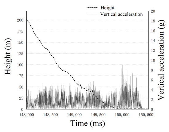
Figure 8.
The vertical acceleration of a hard landing.
In this study, the flight data of 28 sorties of a certain UAV were collected. Multiple landings of the UAV were recorded in one sortie datum. We selected the data of before landing to complete the detection of the fault. A total of 127 representative factors were selected, and 8838 data were obtained. Among them, 432 data failed, and the other 8406 data were normal. The ratio of the fault data to all data was 4.88%. There was a total of 228,600 fault data and 893,826 normal data. For the flight data, the data were preprocessed as per Equation (1). The data were split from the time dimension. In the experiment, the original flight data of each sorting were set as data intervals every .
Some data of the fuel pressure were selected as an example. The wavelet decomposition and reconstruction divide the signal into two parts: low-frequency signal and high-frequency signal. The process of the signal decomposition is shown in Figure 9, in which the results of the first-level decomposition are shown in Figure 9a. The results of the second-level decomposition are shown in Figure 9b. The results of the third-level decomposition are shown in Figure 9c.
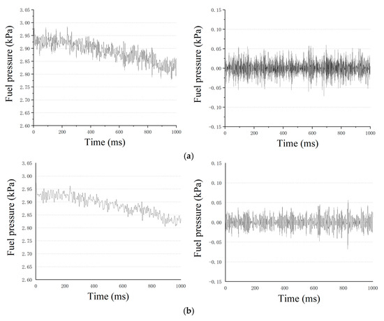
Figure 9.
(a) The high−frequency signal (left) and the low−frequency signal (right) after the first−level decomposition; (b) The high−frequency signal (left) and the low−frequency signal (right) after the second−level decomposition; (c) The high−frequency signal (left) and the low−frequency signal (right) after the third−level decomposition.
In Figure 9, in the process of each level’s decomposition, the signal gradually decomposed by frequency. The high-frequency signal was filtered by wavelet analysis. We believe that the small-amplitude high-frequency signal should not be focused on by the prediction model. Therefore, it was filtered to prevent it from affecting the temporal features extracted by the Auto-Encoder. The time series and the low-frequency signal are shown in Figure 10a,b, respectively.
Figure 10.
(a) Time series; (b) Low-frequency signal.
The filtered small-amplitude high-frequency signal is shown in Figure 11.
Figure 11.
The filtered small−amplitude high−frequency signal.
In Figure 11, the small-amplitude high-frequency signal was similar to the Gaussian signal. There were few valuable features to extract, which will affect the extraction of the temporal features in the signals. In contrast, the low-frequency signal contained almost all of the features of the data and directly determined the trend of the predicted signal. Therefore, the Auto-Encoder should focus on the low-frequency signal. In addition, extracting features according to different frequencies can make the Auto-Encoder pay more attention to important features.
In the UAV Flight Data Sets, the proposed model was used for testing, and different indicators were used for the evaluation to comprehensively evaluate the performance of the model. In the experiment, the label of the fault data was 1 () and the label of the normal data was 0 (). Two-thirds of all data were used for the training set, and the remaining one-third was the test set. The parameters set for the improved Auto-Encoder are shown in Table 2.
Table 2.
The parameters set for the Auto-Encoder.
The parameters of Equation (19) were determined by several experiments. The parameters , , and of Equation (19) are as follows:
The parameters of Equation (23) are as follows:
In the training set, the normal data were used for training, and the reconstruction loss was used as the criterion for fault detection. The impact of the unbalanced data was avoided. We randomly selected two-thirds of the data to train the model and used the remaining data as the test set to verify the effectiveness of the model. There were 171 fault data and 2775 normal data in the verification set.
Accuracy, Precision, Recall, F1 score, and AUC were selected as the evaluation indicators of the model’s predictive ability. The confusion matrix is shown in Table 3.
Table 3.
The confusion matrix.
From Table 3, Accuracy, Precision, Recall, and F1 score are defined by the confusion matrix, as follows [45,46]:
AUC is defined as the area enclosed by the coordinate axis under the ROC curve. The results of the validation set are shown in Table 4.
Table 4.
The results of the validation set.
A variety of fault detection models were selected for comparison, including GBDT, random forest, SVM, RNN, and CNN. The confusion matrix of the GBDT, random forest, SVM, RNN, and CNN are shown in Table 5.
Table 5.
The confusion matrix of the GBDT, random forest, SVM, RNN, and CNN.
The comparison of the verification results of the UAV Flight Data Sets is shown in Table 6.
Table 6.
Comparison of the verification results of the UAV Flight data Sets.
From Table 6, the accuracy of the proposed method was 0.9101. The developed method achieved better results in most situations. The accuracy of the GBDT and random forest was 0.7801 and 0.7410, respectively. They are common ensemble learning models, which improve the classification effect by adding decision trees. The SVM’s accuracy was 0.6167. Generally, the results of the SVM on the small sample training sets were better than the other algorithms. However, the SVM is not suitable for large data sets. It is sensitive to the selection of parameters and kernel functions. The accuracy of the RNN and CNN was 0.8778 and 0.8805, respectively. In the results for the RNN and CNN, there was a low precision and a high recall. Because of the imbalanced data, the feature extraction of the fault data was insufficient. The model has an insufficient ability to identify fault data. The fault data were wrongly detected as normal data [47]. The proposed method alleviates this problem. The developed method uses a large number of normal data in the UAV Flight Data Sets to fully extract the features of normal data. The features of the fault data differed greatly from the normal data. The Auto-Encoder cannot use the features of the fault data for accurate reconstruction. Therefore, accurate fault detection can be achieved by reconstruction loss.
In order to verify the importance of filtering, we used the traditional Auto-Encoder to repeat the experiment. The original data were trained using the traditional Auto-Encoder. The other steps were the same as the developed methods in this paper. The results of both are shown in Table 7.
Table 7.
The results of the developed method and the traditional Auto-Encoder.
From Table 7, the accuracy of the traditional Auto-Encoder was 0.9080. The proposed method achieved better results. The filtering effectively reduced the interference of the high-frequency signal to feature extraction, and important features were extracted.
In order to explore the influence of the number of wavelet layers on the model, the signals filtered by the different number of wavelet layers were tested. The structure of the model is similar to that shown in Figure 5. The only difference is the number of input data frequencies (the model in Figure 5 inputs the data of three frequencies, and the number of wavelet layers is three). Other steps are the same as the developed methods in this paper. In the experiment, the number of wavelet layers were 1, 2, 3, and 4. The results of the experiment are shown in Table 8.
Table 8.
The results of the experiment.
From Table 8, the accuracy of models was 0.9080, 0.9080, 0.9101, and 0.9035. The best number of wavelet layers was three. In addition, with the increase in the number of wavelet layers, the efficiency of the model is improved. We believe that the greater the number of wavelet layers, the more effective the signal filtering. When the number of wavelet layers was four, the accuracy of the model decreased. We believe that too much filtering will cause the loss of important features in the signal.
The efficiency of the developed fault factor location method was verified. The proposed fault factor location method is based on the reconstruction loss of the Auto-Encoder and edge detection operator. The fault data were selected as an example (selected the first of the fault data). in Equation (22) of the fault data is 0.87. The reconstruction loss matrix was obtained by Equation (28). For the reconstruction loss matrix, we should pay attention to the data with large gradient changes. The reconstruction loss matrix is calculated by the edge detection operator, as shown in Equation (25). In order to avoid errors, factors with detection results exceeding are selected. In order to show the data more clearly, visualization of the edge detection results is shown in Figure 12.
Figure 12.
Visualization of the edge detection results.
In Figure 12, some elements in the matrix obviously had large gradients (areas circled in black). A large gradient means that the element has a greater reconstruction loss than the surrounding elements. The factors corresponding to these elements in the matrix cause UAV fault. For example, in the first of the data, the factors that can be detected include temperature of the generator (factor 16), rudder ratio (factor 17), and pitch angle (factor 81). We speculate that it is due to mechanical fatigue and disturbance of external air flow. In order to show the effectiveness of the proposed model more clearly, more results of the experiment are shown in Table 9.
Table 9.
More results of the experiment.
At the end of this study, an explanation is provided for why the proposed model had good results. The traditional fault detection method monitors a certain factor. When it exceeds the safety range, a fault occurs. However, UAVs are complex systems, and faults are caused by multiple factors. In some cases, multiple factors of a UAV are coupled with each other. A fault may occur even if every factor is normal. Traditional methods only focus on the influence of a certain factor on the fault or do not comprehensively consider the coupling of multiple factors. To intuitively illustrate the coupling of multiple factors, the security domain description was used. The security domain of the temperature of the generator and the pitch angle is shown in Figure 13.
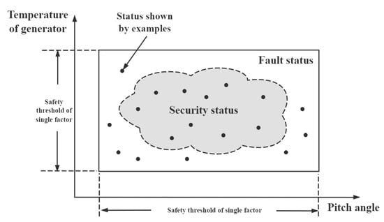
Figure 13.
The security domain of the temperature of the generator and the pitch angle.
In Figure 13, each factor did not exceed the safety range, but the deviation of multiple factors will also cause faults. The proposed model can effectively detect this case.
5. Conclusions
In this study, a new Self-supervised Fault Detection Model for UAVs based on an improved Auto-Encoder was proposed.
In the improved model, only normal data were available as training data to extract the normal features of the flight data and reduce the dimensions of the data. The impact of the unbalanced data was avoided. In the Auto-Encoder, we used wavelet analysis to extract low-frequency signals with different frequencies from the flight data. The Auto-Encoder was used for the feature extraction and reconstruction of low-frequency signals with different frequencies. The high-frequency signal in the data affects the extraction of data features by the Auto-Encoder. Using wavelet analysis to filter noise was helpful for feature extraction. The normal data were used for training. The reconstruction loss was used as the criterion for fault detection. The fault data will produce a higher reconstruction loss. To improve the effectiveness of the fault localization at inference, a novel fault factor location method was proposed. The edge detection operator was used to detect the obvious change of the reconstruction loss, which usually represents the fault factor in the data. The proposed Self-supervised Fault Detection Model for UAVs was evaluated according to accuracy, precision, recall, F1 score, and AUC with the UAV Flight Data Sets. The experimental results show that the developed model had the highest fault detection accuracy among those tested, at 91.01%. Moreover, an explanation of the Self-supervised Fault Detection Model’s results is provided.
It should be noted that only a few fault data were in the data set, and the features of the fault data could not be fully utilized in this study. The Auto-Encoder was used to extract the features of the normal data. In future work, we intend to extract the features of the fault data. In recent years, transfer learning has achieved success in many fields. We intend to analyze the fault data in other data sets through transfer learning. The transferred data can help enrich the features of the fault data. We expect that the full extraction of the fault data features can improve the effectiveness of UAV fault diagnosis. In addition, multiple faults are detected by the proposed model. However, we are unable to explain the reasons for faults caused by multiple factors (it is difficult to explain by the deep learning model), which requires practical and specific analysis. Using the deep learning model to explain the mechanism of a fault is also a future research direction.
In summary, this study analyzed the features of UAV Flight Data Sets and proposed a novel Self-supervised Fault Detection Model for UAVs. The proposed model had a better performance.
Author Contributions
Conceptualization, S.Z.; data curation, T.W. and L.Y.; formal analysis, T.W.; funding acquisition, S.Z. and S.C.; investigation, T.W. and Z.H.; methodology, S.Z. and Z.H.; project administration, T.W.; resources, S.C.; supervision, S.Z.; validation, T.W. and L.Y.; visualization, Z.H. and T.W.; writing—original draft, T.W.; writing—review and editing, T.W. All authors have read and agreed to the published version of the manuscript.
Funding
This research was funded by the National Natural Science Foundation of China (Grant No. 71971013) and the Fundamental Research Funds for the Central Universities (YWF-22-L-943). The study was also sponsored by the Graduate Student Education and Development Foundation of Beihang University.
Institutional Review Board Statement
Not applicable.
Informed Consent Statement
Not applicable.
Data Availability Statement
Not applicable.
Acknowledgments
All authors would like to thank those who provided support through funding.
Conflicts of Interest
The authors declare no conflict of interest.
References
- Yang, L.; Jia, G.; Wei, F. The CIPCA-BPNN failure prediction method based on interval data compression and dimension reduction. Appl. Sci. 2021, 11, 3448. [Google Scholar] [CrossRef]
- Turan, V.; Avar, E.; Asadi, D. Image processing based autonomous landing zone detection for a multi-rotor drone in emergency situations. Turk. J. Eng. 2021, 5, 193–200. [Google Scholar] [CrossRef]
- Asadi, D.; Ahmadi, K.; Nabavi-Chashmi, S. Controlability of multi-rotors under motor fault effect. Artıbilim: Adana Alparslan Türkeş Bilim Ve Teknol. Üniversitesi Fen Bilim. Derg. 2021, 4, 24–43. [Google Scholar]
- Huang, C.; Xu, Q.; Wang, Y. Self-Supervised Masking for Unsupervised Anomaly Detection and Localization. IEEE Trans. Multimed. 2022. [Google Scholar] [CrossRef]
- Gordill, J.D.; Celeita, D.F.; Ramos, G. A novel fault location method for distribution systems using phase-angle jumps based on neural networks. In Proceedings of the 2022 IEEE/IAS 58th Industrial and Commercial Power Systems Technical Conference (I&CPS), Las Vegas, NV, USA, 1–5 May 2022; pp. 1–6. [Google Scholar]
- Chen, Y.; Liu, Y.; Jiang, D. Sdae. Self-distillated masked autoencoder. In Proceedings of the European Conference on Computer Vision, Tel Aviv, Israel, 23–24 October 2022; pp. 108–124. [Google Scholar]
- Zhou, S.; Wei, C.; Li, P. A Text-Driven Aircraft Fault Diagnosis Model Based on Word2vec and Stacking Ensemble Learning. Aerospace 2021, 8, 357. [Google Scholar] [CrossRef]
- Luo, M.; Li, C.S.; Zhang, X.Y.; Li, R.H.; An, X.L. Compound feature selection and parameter optimization of ELM for fault diagnosis of rolling element bearings. Isa Trans. 2016, 65, 556–566. [Google Scholar] [CrossRef] [PubMed]
- Li, C.; Sanchez, R.V.; Zurita, G.; Cerrada, M.; Cabrera, D.; Vasquez, R.E. Gearbox fault diagnosis based on deep random forest fusion of acoustic and vibratory signals. Mech. Syst. Signal Process. 2016, 76–77, 283–293. [Google Scholar] [CrossRef]
- Cheng, G.; Chen, X.H.; Li, H.Y.; Li, P.; Liu, H.G. Study on planetary gear fault diagnosis based on entropy feature fusion of ensemble empirical mode decomposition. Measurement 2016, 91, 140–154. [Google Scholar] [CrossRef]
- Meng, Z.; Huo, H.; Pan, Z. A gear fault diagnosis method based on improved accommodative random weighting algorithm and BB-1D-TP. Measurement 2022, 195, 111169. [Google Scholar] [CrossRef]
- Gao, K.; Xu, X.; Li, J. Weak fault feature extraction for polycrystalline diamond compact bit based on ensemble empirical mode decomposition and adaptive stochastic resonance. Measurement 2021, 178, 109304. [Google Scholar] [CrossRef]
- Shao, Y.; Du, S.; Tang, H. An extended bi-dimensional empirical wavelet transform based filtering approach for engineering surface separation using high definition metrology. Measurement 2021, 178, 109259. [Google Scholar] [CrossRef]
- Liu, Q.; Yang, J.; Zhang, K. An improved empirical wavelet transform and sensitive components selecting method for bearing fault. Measurement 2022, 187, 110348. [Google Scholar] [CrossRef]
- Zhang, Y.; Zhang, L. Intelligent fault detection of reciprocating compressor using a novel discrete state space. Mech. Syst. Signal Process. 2022, 169, 108583. [Google Scholar] [CrossRef]
- Li, Y.; Ma, F.; Ji, C. Fault Detection Method Based on Global-Local Marginal Discriminant Preserving Projection for Chemical Process. Processes 2022, 10, 122. [Google Scholar] [CrossRef]
- Long, Z.; Zhang, X.; He, M. Motor fault diagnosis based on scale invariant image features. IEEE Trans. Ind. Inform. 2021, 18, 1605–1617. [Google Scholar] [CrossRef]
- Zhang, Y.; Han, Y.; Wang, C. A dynamic threshold method for wind turbine fault detection based on spatial-temporal neural network. J. Renew. Sustain. Energy 2022, 14, 053304. [Google Scholar] [CrossRef]
- Su, N.; Zhou, Z.J.; Zhang, Q. Fault Feature Extraction of Bearings for the Petrochemical Industry and Diagnosis Based on High-Value Dimensionless Features. Trans. FAMENA 2022, 46, 31–44. [Google Scholar] [CrossRef]
- Lei, D.; Chen, L.; Tang, J. Mining of Weak Fault Information Adaptively Based on DNN Inversion Estimation for Fault Diagnosis of Rotating Machinery. IEEE Access 2021, 10, 6147–6164. [Google Scholar] [CrossRef]
- Fu, Y.; Chen, X.; Liu, Y. Gearbox Fault Diagnosis Based on Multi-Sensor and Multi-Channel Decision-Level Fusion Based on SDP. Appl. Sci. 2022, 12, 7535. [Google Scholar] [CrossRef]
- Deng, W.; Yao, R.; Zhao, H. A novel intelligent diagnosis method using optimal LS-SVM with improved PSO algorithm. Soft Comput. 2019, 23, 2445–2462. [Google Scholar] [CrossRef]
- Jahromi, A.T.; Er, M.J.; Li, X. Sequential fuzzy clustering based dynamic fuzzy neural network for fault diagnosis and prognosis. Neurocomputing 2016, 196, 31–41. [Google Scholar] [CrossRef]
- Amozegar, M.; Khorasani, K. An ensemble of dynamic neural network identifiers for fault detection and isolation of gas turbine engines. Neural Netw. 2016, 76, 106–121. [Google Scholar] [CrossRef]
- Wang, K.; Guo, Y.; Zhao, W. Gas path fault detection and isolation for aero-engine based on LSTM-DAE approach under multiple-model architecture. Measurement 2022, 202, 111875. [Google Scholar] [CrossRef]
- Liu, X.; Liu, S.; Xiang, J. An ensemble and shared selective adversarial network for partial domain fault diagnosis of machinery. Eng. Appl. Artif. Intell. 2022, 113, 104906. [Google Scholar] [CrossRef]
- Sun, R.; Liu, X.; Liu, S. A game theory enhanced domain adaptation network for mechanical fault diagnosis. Meas. Sci. Technol. 2022, 33, 115501. [Google Scholar] [CrossRef]
- Han, T.; Liu, C.; Wu, L. An adaptive spatiotemporal feature learning approach for fault diagnosis in complex systems. Mech. Syst. Signal Process. 2019, 117, 170–187. [Google Scholar] [CrossRef]
- Su, Z.; Tang, B.; Liu, Z. Multi-fault diagnosis for rotating machinery based on orthogonal supervised linear local tangent space alignment and least square support vector machine. Neurocomputing 2015, 157, 208–222. [Google Scholar] [CrossRef]
- Yuan, J.; Zhao, R.; He, T. Fault diagnosis of rotor based on Semi-supervised Multi-Graph Joint Embedding. ISA Trans. 2022, 131, 516–532. [Google Scholar] [CrossRef] [PubMed]
- Zhou, S.; Qian, S.; Chang, W. A novel bearing multi-fault diagnosis approach based on weighted permutation entropy and an improved SVM ensemble classifier. Sensors 2018, 18, 1934. [Google Scholar] [CrossRef]
- Zhou, S.; Qian, S.; Qiao, X. The UAV landing quality evaluation research based on combined weight and VIKOR algorithm. Wirel. Pers. Commun. 2018, 102, 2047–2062. [Google Scholar] [CrossRef]
- Zhang, M.; Kong, P.; Hou, A. Identification Strategy Design with the Solution of Wavelet Singular Spectral Entropy Algorithm for the Aerodynamic System Instability. Aerospace 2022, 9, 320. [Google Scholar] [CrossRef]
- Du, X.; Chen, J.; Zhang, H. Fault Detection of Aero-Engine Sensor Based on Inception-CNN. Aerospace 2022, 9, 236. [Google Scholar] [CrossRef]
- Swinney, C.J.; Woods, J.C. Unmanned aerial vehicle operating mode classification using deep residual learning feature extraction. Aerospace 2021, 8, 79. [Google Scholar] [CrossRef]
- Asadi, D. Model-based fault detection and identification of a quadrotor with rotor fault. Int. J. Aeronaut. Space Sci. 2022, 23, 916–928. [Google Scholar] [CrossRef]
- Asadi, D. Partial engine fault detection and control of a Quadrotor considering model uncertainty. Turk. J. Eng. 2022, 6, 106–117. [Google Scholar] [CrossRef]
- Hu, C.; Liu, M.; Li, H. Sliding Mode Observer-Based Stuck Fault and Partial Loss-of-Effectiveness (PLOE) Fault Detection of Hypersonic Flight Vehicle. Electronics 2022, 11, 3059. [Google Scholar] [CrossRef]
- Wen, Y.; Ye, X.; Su, X. Event-Triggered Fault Detection Filtering of Fuzzy-Model-Based Systems with Prescribed Performance. IEEE Trans. Fuzzy Syst. 2022, 30, 4336–4347. [Google Scholar] [CrossRef]
- Shu, Z.; Sahasrabudhe, M.; Guler, R.A.; Samaras, D.; Paragios, N.; Kokkinos, I. Deforming autoencoders: Unsupervised disentangling of shape and appearance. In Proceedings of the European Conference on Computer Vision (ECCV), Munich, Germany, 8–14 September 2018; pp. 650–665. [Google Scholar]
- Jing-Yi, L.; Hong, L.; Dong, Y. A new wavelet threshold function and denoising application. Math. Probl. Eng. 2016, 2016, 3195492. [Google Scholar] [CrossRef]
- Zhu, L.; Bao, S.H.; Qiu, L.P. Simple Algorithm of Wavelet Decomposition Depth and Program Realization. Trans. Tech. Publ. Ltd. 2012, 472, 2231–2234. [Google Scholar]
- Boggess, A.; Narcowich, F.J. A First Course in Wavelets with Fourier Analysis; John Wiley & Sons: Hoboken, NJ, USA, 2015. [Google Scholar]
- Chetia, R.; Boruah, S.M.B.; Sahu, P.P. Quantum image edge detection using improved Sobel mask based on NEQR. Quantum Inf. Process. 2021, 20, 1–25. [Google Scholar] [CrossRef]
- Mitra, B.; Craswell, N. An introduction to neural information retrieval. Found. Trends Inf. Retr. 2018, 13, 1–126. [Google Scholar] [CrossRef]
- Fernández, J.C.; Carbonero, M.; Gutiérrez, P.A. Multi-objective evolutionary optimization using the relationship between F1 and accuracy metrics in classification tasks. Appl. Intell. 2019, 49, 3447–3463. [Google Scholar] [CrossRef]
- Wei, C.; Sohn, K.; Mellina, C. Crest: A class-rebalancing self-training framework for imbalanced semi-supervised learning. In Proceedings of the IEEE/CVF Conference on Computer Vision and Pattern Recognition, Nashville, TN, USA, 19–25 June 2021; pp. 10857–10866. [Google Scholar]


Disclaimer/Publisher’s Note: The statements, opinions and data contained in all publications are solely those of the individual author(s) and contributor(s) and not of MDPI and/or the editor(s). MDPI and/or the editor(s) disclaim responsibility for any injury to people or property resulting from any ideas, methods, instructions or products referred to in the content. |
© 2023 by the authors. Licensee MDPI, Basel, Switzerland. This article is an open access article distributed under the terms and conditions of the Creative Commons Attribution (CC BY) license (https://creativecommons.org/licenses/by/4.0/).