UltraFLoads: A Simulation Suite and Framework for High-Fidelity Flight Loads

Abstract

With the progress of high-performance computing, computationally expensive high-fidelity methods can be applied early in the design process of an aircraft. This enables Computational Fluid Dynamics (CFD) for the assesment of flight performance, handling qualities, flight loads due to manoeuver or gusts, and stability such as flutter. Those aeroealstic analyses require coupling of disciplines to adequately address the interplay of flexibility, aerodynamic forces and inertia forces. Previous work at the German Aerospace Center have demonstrated the proof of concept for those multidisciplinary analyses. Now, UltraFLoads is a simulation suite in the FlowSimulator ecosystem to offer standardized, multidisciplinary scenarios. UltraFLoads can be used as a tool, as a library and as a framework. This work describes the architecture, the integration layers, which scenarios are available and which equations are used. Three different applications are presented. The first case involves a steady fluid–structure-coupled simulation with geometrically nonlinear deformation. The second case compares the deformation of a simulated elastic, free-flying aircraft with actual flight test data. The last application demonstrates the flight dynamic capabilities with a bank to bank maneuver.

1. Introduction

Certification for transport aircraft (CS25, [1]) prescribe that flight loads due to maneuvers, gust encounters or continuous turbulence need to be considered. Flexible wing structures lead to interaction between the flow and the deformation of the wing, which result in different load distributions. Therefore, the calculations must couple the aerodynamic, structural and flight mechanic disciplines, which is the field of aeroelasticity.

With the progress of high-performance computing and advances in high-fidelity simulations with Computational Fluid Dynamics (CFD), virtual prototyping has become a reality for aircraft design. CFD in gust and maneuver loads computations enrich modern aircraft design, because it may include viscous, compressible and rotational flow and less simplifications about the geometric representation are necessary. Compared to industrialized lower-fidelity methods, those simulations quickly become complex, time consuming and need to be solved in a multiprocessing HPC environment. Software for each discipline has been matured and combined in multi-disciplinary simulation, with the challenge to scale well for systems of equations with millions of unknowns.

The solver for high-fidelity aerodynamic simulations is currently the DLR TAU-Code [2]. In the near future the solver will be replaced by the next-generation CFD solver CODA, which descends from DLR’s solver prototype implementation Flucs [3]. CODA is currently being diligently developed in a joint effort by DLR, Airbus and ONERA. The FlowSimulator DataManager (FSDM) [4], jointly developed by DLR, Airbus and ONERA, provides an HPC library for CFD-based simulation workflows, data models, data manipulation and multiprocessing. As the core library includes Python interfaces, additional convenient control layers (FSDLRControl, FSControl) have been developed to organize data and workflows in Python. Those layers simplify the volume mesh deformation, interaction with TAU, MSC.Nastran, B2000++ pro (https://www.smr.ch/products/b2000/, accessed on 14 December 2022) and many more. As the FSDM ecosystem is highly modularized and a centralized data model is available, each user or researcher can combine the data and methods individually for their needs. This was used for example in a proposed approach by Backhaus et al. [5], where the optimization capabilities of OpenMDAO (https://openmdao.org/, accessed on 14 December 2022) [6] are combined with the FSDM.

Flight loads, performance evaluations, flutter analysis, buffeting, divergence, reversal of control are characterized by their interaction between aerodynamic, elastic and inertia forces [7]. As a consequence, every software which provides the analysis capabilities for those aeroelastic problems needs to adequately address coupling of disciplines. For fully linear methods, all disciplines can be coupled monolithicaly in one system of equations and solved directly, for which MSC.Nastran [8] is a good example. The combination of different software tools for each disciplines does not necessarily allow such a tight coupling. Other codes like SHARPy [9] or UM/Nast [10] are specialized for very flexible and slender aircraft which require nonlinear structural mechanics using beam models which are coupled to aerodynamic potential flow models. Thus, those codes require an additional step to determine the beam properties based on a more complex finite element model with different types of elements. The Loads Kernel [11] provides time-domain and frequency domain aeroelastic simulations for maneuver, gust and flutter simulation. Furthermore, it has been coupled to the DLR TAU-Code directly but does not use the FlowSimulator environment and therefore cannot include all the new features and libraries which are developed solely within the FlowSimulator.

Another prototypical code has demonstrated and progressed the capability of high-fidelity flight dynamic simulations for fully flexible, free-flying aircraft [12,13]. This prototype already works with the FlowSimulator, but it is more a collection of scripts for each scenario, making it hard to maintain and further develop. Now, this predecessor is being replaced by a new software called UltraFLoads. UltraFLoads uses the FlowSimulator ecosystem and the software itself is available to all researchers at the DLR. Due to the increasing number of researchers using high-fidelity simulations, the interest in UltraFLoads is growing and therefore more scientific results will be based on this framework.

The requirements are that the software must be flexible as modifications and new methods are developed or investigated in a scientific research environment. Furthermore, the new loads framework comprises multiple sets of simulations like trimmed steady maneuver loads, unsteady maneuvers and gust encounters. For all of those scenarios, aerodynamic solvers of various fidelity levels, trim algorithms and coupling strategies need to be available. Furthermore, researchers frequently need to implement new methods to answer new questions. Thus, prototypical programming must be possible using the framework. As multiple levels of fidelities are requested for loads computation, the name of the framework is ultra fidelity loads or short UltraFLoads. The framework has already been used for high-fidelity loads computation for quasi-steady pull-up and roll-maneuvers [14], the architecture is described in [15], and recent investigations on nonlinear aerodynamics coupled with geometrically nonlinear structural mechanics demonstrated the capabilities of UltraFLoads [16].

This paper shows which equations are implemented, how the analyses are combined, which capabilities exists and what will be implemented. Finally, three cases are demonstrated. One case, to show the need for coupling nonlinear aerodynamics with nonlinear structural mechanics, based on the work of [16]. A second validation case, to show good agreement of the computed and measured deformation of the research aircraft DLR-ATRA (A320-232) in a steady turn [15]. The final case shows the capabilities of the new flight dynamic solver, by performing a rigid, bank-to-bank maneuver with the new research aircraft DLR-ISTAR (Dassault Falcon 2000LX).

2. Technical Context

2.1. FlowSimulator DataManager

The FSDM is an open software platform, jointly developed by Airbus, Onera and DLR for high fidelity simulations involving CFD [4,17]. It provides a framework for scalable parallel computations on high performance computers.

The FSDM objects are for example integer, float and string arrays, datasets, mesh objects and a data manager object with a registry for FSDM data objects. Knowing the keys for arrays or meshes allows to receive those data objects anywhere in the process from the data manager object. To organize additional information about the data and the relations of them, a so called relations model is accessible via each data manager object as well. It is a hierarchical data model, which can be imported/exported from/to XML format. Furthermore, float arrays can be monitored in a data logger, which is structured in categories and quantity names. The relations model is therefore a good candidate to store additional information, settings and monitoring in one place. It can be used as tool input, tool output, online monitoring and is a simple solution for restarting or continuing a simulation. So the data manager object provides access to arrays, meshes and the relations model. Thus, the data manager object is most of the time used as a global object, which is passed to plug-ins and functions.

The mesh objects can be imported from and exported to different mesh file types (NetCFD, CGNS, HDF5, Tecplot). Furthermore, a variety of partitioning methods like Zoltan [18] or ParMetis [19] can be applied to mesh objects for parallel applications.

All C++ objects are wrapped to Python by using the Simplified Wrapper and Interface Generator (SWIG) (https://www.swig.org/, accessed on 14 December 2022) to enable Python as integration environment.

Another layer of the FlowSimulator is the plug-in layer. Mesh manipulation, flow solver, structural solver, trim solver, etc. are separated plug-ins which can work with the FlowSimulator data and communication objects. Since the data manager object can be used as a global object, each plug-in can work with this object leading to stateless designs in many cases. To ease the interactions with the plug-ins, several Python based wrapper classes are available. For example, one volumetric mesh deformation plug-in can be used differently to allow for a mesh morphing based control surface deflection [4] or to rotate the tail plane.

The top layer is the integration layer, where the scenarios are defined. The interaction of plug-ins, control objects and data objects have to be orchestrated by the user. Depending on the problem of interest, a specific simulation and hence a specific scenario is required. This has led to collections of python scripts for specific scenarios. With the increasing number of of applications, tools and combination possibilities, a generator for scenarios is useful. One approach for a generator for scenarios is to provide scenarios using the openMDAO framework together with the FlowSimulator [5].

2.2. DLR Tau-Code

One of DLR’s CFD solvers is the DLR Tau-Code for solving the unsteady Reynolds-Averaged Navier–Stokes equations and various turbulence models. It is suitable for simulation of transport aircraft in transonic flow. Tau is an edge-based unstructured solver, using the dual-grid approach and works with hybrid meshes.

For this paper only a subset of Tau’s capabilities are depicted, which are necessary for flight dynamic simulation with moving meshes. Further details can be found in [2,20].

An arbitrary Euler Lagrangian (ALE) formulation is used to allow for Euler and Lagrangian perspective. Rigid body motion and or mesh deformation can be considered for the grid movement. The mesh deformation results from control surface deflections, tail plane rotations and structural deformations. The rigid body motion can be described by position, Euler angles, translatory and rotatory velocity components. The rigid body motion is based on a hierarchical node system with kinematic relations, where each node controls different blocks of the computational domain. Each motion can be controlled via an external motion module using Python. With the motion nodes, the grid velocities can be computed to account for all translatory and rotatory degrees of freedom of the aircraft in flight dynamic simulations.

Engine intake and outtake boundary patches can be defined to include more realistic engine effects in the simulation. This can be achieved by different combinations of prescribing thermodynamic states or thermodynamic ratios on the inlet and outlet boundaries.

The Tau-Code can be used for steady and unsteady simulations and allows to control advancing in time, which enables predictor-corrector time integration schemes.

2.3. Volumetric Mesh Deformation

The FlowSimulator provides plug-ins for mesh deformation. There is one strategy based on a structural elasticity analogy [21,22] and one which is based on three dimensional radial basis functions [23,24]. In both cases, the deformation of the surface nodes are propagated into the volumetric mesh. The elastic approach uses all surface nodes and may become computationally expensive for large systems. The radial basis method can use a reduction method to reduce the number of base nodes to be computationally efficient. A common technique is to deform the whole domain with the radial basis approach and if the volumes of some cells become negative, the elastic approach is applied as repair step in a small region around the negative volumes [4].

The mesh morphing approach in [4] is applied for control surface deflections. For the rotation of the trim surfaces, a FlowSim plug-in is used as well. Here, the no-normal-movement constraint is applied, which ensures that other surface nodes, for example on the fuselage, do not move out of their normal-plane.

The deformation of the volumetric mesh results from the sequential execution of control surface deflection, tail plane rotation and elastic deformation. In case of cells with negative volumes, the mesh repair algorithm is executed.

3. UltraFLoads

UltraFLoads is a simulation suite to provide scenarios to researchers in the FlowSimulator context. It is designed for several use cases. A command line tool is provided which can interpret a simplified input and execute simulations. Thus, the user does not need to know implementation details or know Python. Other users can use UltraFLoads as a library to integrate analysis classes in their own scripts. Or, UltraFLoads can be used as a framework, so user defined analysis can be injected in the simulation scenarios as well. The architecture of UltraFLoads is outlined in [15].

Each scenario is implemented as an analysis class, which inherits from the same interface class. The base interface is extended by additional abstract methods for each disciplinary interface. For example, aerodynamic analyses must have a method to get the surface forces whether it is based on a lower-fidelity method or a wrapper to Tau or CODA. The dependency inversion and dependency injection technique is used for multi-disciplinary or nested analysis interfaces. For example, a concrete aerodynamic and a concrete structural analysis can be used in a concrete aero-structural analysis as they implement the aerodynamic and structural interfaces.

All analysis instances require a data manager object and all the information needed to run the simulation are stored in the relations model. Since the relations model is hierarchic, one can easily segregate information for different tasks. An exemplary structure of the relations model is provided below.

■

/MESHES/A320

●

Parameters

✧

Mesh key: CFDMesh

✧

Import type: HDF5

■

/CFD/TAU

●

Parameters

✧

Mesh key: CFDMesh

❍

DataLog

★

Monitoring

✩

$C_L$: [0.3, 0.32, 0.4, …]

■

/SIXDOF

●

Parameters

✧

Analysis key: TAU

❍

DataLog

★

Monitoring

✩

$n_z$: [0.8, 0.82, 1.1, …]

So there is one domain (■) for mesh related information, one domain for rigid body motion, one domain for TAU and so on. All information are stored centrally in the relations model and the plug-ins can use it to exchange data.

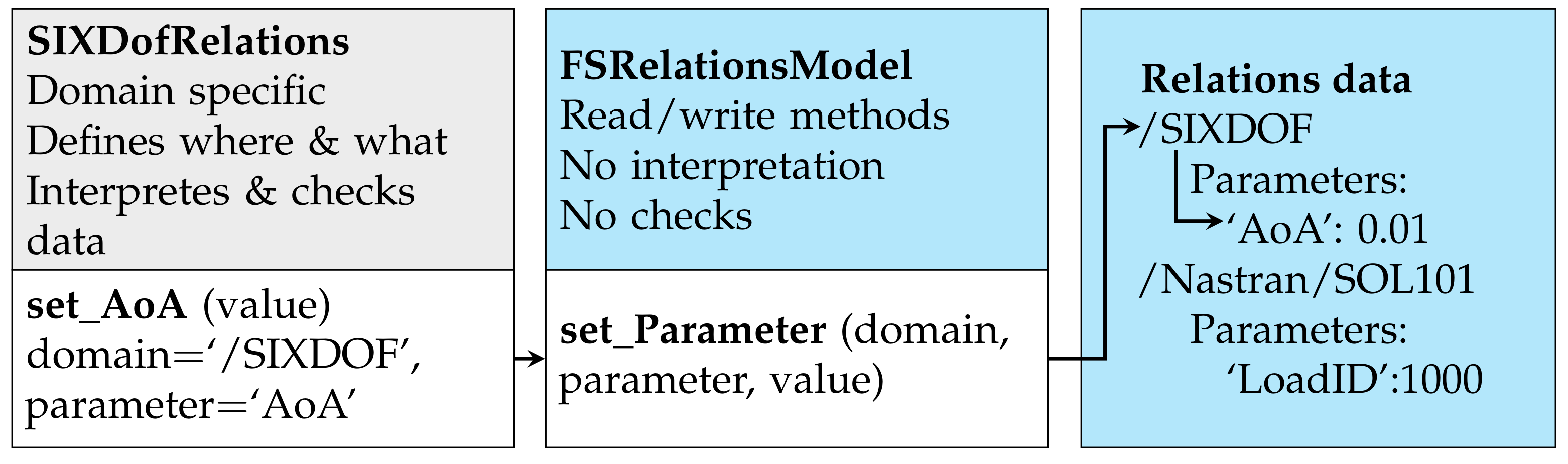
Python wrapper classes for each domain are introduced to ease the interaction with the relations model. Thus, instead of interacting with the relations model directly, which requires to know the name of the domain and the name of parameter (●), the user or developer can simply set the angle of attack via the wrapper object as shown in Figure 1. As those wrapper instances do not have any state and depend solely on the data manager, they can be constructed easily. To receive information about any analysis object, the corresponding relations wrapper for that domain can be used. This is especially useful for post-processing of the relations-model, where the analysis object may not exist anymore.

The relations model can be written to disk at runtime, so the user can monitor the data, already do some post-processing and use it as restart for other simulations. This is especially of value for high-fidelity simulations which run for days and therefore need some kind of online-monitoring. As the relations model can become very detailed, it is a good documentation of what has been simulated and how the simulation has been configured. This helps for archiving, inspections and debugging. The interplay between relations interface is exemplified for the analysis class for TAU in Figure 2. The analysis class orchestrates the different FlowSimulator plugins and receives the necessary information from the relations model.

There is one analysis class registry, from which each analysis can be imported from using a key. User can register own analysis classes with a user defined key. An analysis factory can then create analysis objects using the class registry and the information stored in the relations model. For example, the aero-structural solver could use any aerodynamic or structural analysis object. It is up to the user to decide, which key should be used for the aerodynamic analysis and which key for the structural analysis. The currently available analysis classes in UltraFLoads are:

• Aerodynamic analysis wrapper for TAU;
• Aerodynamic analysis based on aerodynamic coefficients;
• Two structural analysis wrapper of MSC.Nastran for SOL101 and SOL400;
• Steady structural analysis based on linear vibration modes;
• Steady aero-structural analysis, loosely coupled and sequentially solved;
• Quasi-steady rigid body motion analysis;
• Trim analysis to determine control values for a target state, solved by a damped Gauss–Newton solver;
• Unsteady aerodynamic solver coupled to linear vibration modes, solved by an ODE solver;
• Unsteady rigid body flight dynamics solved by an ODE solver;
• Unsteady flight dynamics analysis with linear free vibration modes and mean axis assumption, solved by an ODE solver;
• Single parameter sweep analysis for parameter variation studies.

All discrete models are represented as mesh objects of the FlowSimulator, which eases the usage of other FlowSimulator libraries. Furthermore, the FlowSimulator plug-ins are used as much as possible to reuse work of other researchers, which improves the overall code quality but introduces challenges for the software development and integration.

3.1. Actuators and Control

Actuators and controls are defined in the relations model and are the variables which alter the behavior of the disciplines. For example, the angle of attack is varied to change the lift coefficient in a trim scenario. Some control surfaces need to be controlled by a flight control system and other actuators might follow a predefined signal to introduce disturbances on the system. The different use cases are:

• Rigid body motion actuators to modify Euler angles and body speeds;
• Rigid body force actuator to mimic artificial forces like thrust;
• Force field actuator to scale a force field to compensate for missing components;
• Control surface actuators;
• Engine actuators.

Each actuator has a state, a lower limit and an upper limit. The state is then used by wrapper for plug-ins, which have additional information stored for the actuators. A control surface actuator state is used together with the information stored in the relations wrapper for the volumetric mesh deformation. Those additional information are hinge-point positions, which parts of the mesh should be affected, how large the blending radius should be, etc. The actuator and the control surface definition are then matched by their name, so the volume mesh deformation wrapper can receive the state and deform the mesh accordingly. Furthermore, each actuator may have a prescribed time signal, which can be relative or absolute to an initial state. Depending on the physical time, which is centrally stored in the relations model as well, the actuator is forced to return the value of the signal. This allows to introduce disturbances for examples for control surface deflections.

Additionally, control variables $\mathit{x}$ are introduced, where each variable may alter multiple actuators $\mathit{\xi }$ with different participation factors $\mathit{P}$. Thus, the relation from controls to actuator is

$$\mathit{\xi }=\mathit{P}\mathit{x}.$$

(1)

For example a pilot roll command may modify the state of the inner and outer ailerons differently and have different signs for the left and the right ailerons. The participation factors can be modified as well, which might be needed for controlled flight dynamics with malfunctioning controls.

3.2. Trim Solver

For Quasi-steady maneuvers the forces and moments acting on the aircraft must be balanced such that the accelerations are zero. This state is referred to as trimmed state. However, the required inputs to reach the steady state are unknown and need to be solved by a trim solver. The aircraft trim problem can be seen as a root finding problem or a minimization problem with $\mathit{x}$ as inputs, $\mathit{y}$ as outputs and $\widehat{\mathit{y}}$ as target output. A general solution the aircraft trim problem is shown in [25].

UltraFLoads views the trim problem also as a general minimization problem of an objective $f\left(\mathit{x}\right)$ using the output residual $\mathit{r}\left(\mathit{x}\right):=\widehat{\mathit{y}}-\mathit{y}\left(\mathit{x}\right)$

$$f\left(\mathit{x}\right)=\frac{1}{2}\mathit{r}{\left(\mathit{x}\right)}^T\mathit{r}\left(\mathit{x}\right).$$

(2)

A minimization problem can be solved by optimization algorithms, which may consider bounding box constraints on the inputs $\mathit{x}$, equality constraints, or inequality constraints. UltraFLoads provides a damped Gauss–Newton solver for unconstrained, determined systems, meaning the number of target outputs must match the number of input variables. A search direction s is scaled and added to the input during the line search.

$${\mathit{x}}^{(l+1)}={\mathit{x}}^{\left(l\right)}+\alpha {\mathit{s}}^{\left(l\right)}$$

(3)

The search direction is determined by the gradient ${\mathit{g}}^{\left(l\right)}:=\nabla f\left({\mathit{x}}^{\left(l\right)}\right)$ and the Hessian ${\mathit{H}}^{\left(l\right)}:={\nabla }^{2}f\left({\mathit{x}}^{\left(l\right)}\right)$ of the objective function [26].

$${\mathit{H}}^{\left(l\right)}{\mathit{s}}^{\left(l\right)}=-{\mathit{g}}^{\left(l\right)}$$

(4)

The gradient $\nabla f$ depends on the Jacobian $J_{ij}=\partial r_i/\partial x_j$ of the output residual for the quadratic problem in Equation (2)

$$\nabla f^{\left(l\right)}={{\mathit{J}}^{\left(l\right)}}^T\mathit{r}\left({\mathit{x}}^{\left(l\right)}\right).$$

(5)

The Hessian ${\nabla }^{2}f$ is only approximated by the Jacobian

$${\nabla }^2{f}^{\left(l\right)}\approx {{\mathit{J}}^{\left(l\right)}}^T{\mathit{J}}^{\left(l\right)}.$$

(6)

The value for $\alpha$ can be provided by a user supplied sequence, or using Aitken relaxation [27] or determined by the Armijo Linesearch algorithm. For the first iterations it is usually $\alpha <1$ and close to the solution $\alpha =1$ [26].

The initial Jacobian ${\mathit{J}}^{\left(0\right)}$ can be user provided as well. The Jacobian is calculated by forward finite differences, which can become inefficient for many inputs. To reduce computational time, the initial Jacobian for the initial variables ${\mathit{x}}^{\left(0\right)}$ can be used for all iterations

$${\mathit{J}}^{\left(l\right)}\approx {\mathit{J}}^{\left(0\right)}.$$

(7)

The trim solver can work with analysis objects, which implement the base analysis interface. The possible inputs for the trim solver are control variables which are defined in Section 3.1. The user has to select the target outputs and the analysis. For example, if one wants to trim an aircraft to reach a lift coefficient by altering the angle of attack, an aerodynamic analysis can be used. However, if the goal is to trim the aircraft to a target load factor, an aerodynamic analysis will not work as a load factor is not defined in the aerodynamic analysis. Instead, a flight mechanic analysis is required since the load factor is based on the rigid body acceleration, which requires information about the mass, the center of gravity and the integrated loads at the center of gravity.

3.3. Solving First Order Ordinary Differential Equations

Many time evolving problems in engineering can be written as first order, ordinary differential Equations (ODE)

$$\dot{\mathit{y}}=\mathit{f}(t,\mathit{y}).$$

(8)

For example, the second order differential equation of motion for flight dynamics with and without elastic degrees of freedom can be written as first order ordinary differential Equation [28].

Those equations can be solved numerically by the Runge–Kutta methods or linear multistep methods. The Adams-Moulton method is an implicit linear multistep method, for which a predictor-evaluate-corrector-evaluate (PECE) schema can be applied [29]. The approach is implemented in UltraFLoads and is outlined in Algorithm 1. The maximum number of corrector-evaluate steps can be controlled by the user. Setting it to zero will result in an explicit Adams–Bashforth method.

Algorithm 1 Implicit multistep solver for first order ODE

Require:$\mathit{f}(t,\mathit{y})$  function Integrate($\mathit{f}$, N, $NC$, $\Delta t$)       ▹N: multi steps, $NC$: correction steps, $\Delta t$: time step size   $t_{i+1}=t_i+\Delta t$   ${\dot{\mathit{y}}}_{i+1,\mathrm{predict}}\leftarrow \mathrm{adamsbashforth}\left([{\dot{\mathit{y}}}_i,\dots ,{\dot{\mathit{y}}}_{i-N}]\right)$   ${\mathit{y}}_{i+1}\leftarrow {\mathit{y}}_i+\Delta t{\dot{\mathit{y}}}_{i+1,\mathrm{predict}}$                          ▹ Predict   ${\dot{\mathit{y}}}_{i+1}\leftarrow \mathit{f}(t_{i+1},{\mathit{y}}_{i+1})$                         ▹ Evaluate   for $k\leftarrow 0$ to $NC$ do      ${\dot{\mathit{y}}}_{i+1,\mathrm{correct}}\leftarrow \mathrm{adamsmoulton}\left([{\dot{\mathit{y}}}_{i+1},\dots ,{\dot{\mathit{y}}}_{i-N-1}]\right)$      ${\mathit{y}}_{i+1}\leftarrow {\mathit{y}}_i+\Delta t{\dot{\mathit{y}}}_{i+1,\mathrm{correct}}$                       ▹ Correct      ${\dot{\mathit{y}}}_{i+1}\leftarrow \mathit{f}(t_{i+1},{\mathit{y}}_{i+1})$                       ▹ Evaluate   end for end function

The start up problem is solved with lower order multi-step methods. This leads to larger errors, if the system is not steady at the start. More accurate start up strategies will be implemented in the future.

3.4. Modal Approach

Linear structural dynamics can be described by a reduced order model based on superposition of a selection of normal modes $\mathbf{\Phi }$, the generalized coordinates $\mathit{\eta }$ and structural eigenvalues ${\omega }^2$ [30]. The structural deformation $\mathit{u}$ are then substituted by $\mathit{u}=\mathbf{\Phi }\mathit{\eta }$. The equation of motion without damping with excitation loads $\mathit{b}$ reads then

$$\mathit{M}\mathbf{\Phi }\ddot{\mathit{\eta }}+\mathit{K}\mathbf{\Phi }\mathit{\eta }=\mathit{b}$$

(9)

Having mass normalized modes, the equation can be multiplied by the transpose of the modes.

$$\underset{\mathit{I}}{\underbrace{{\mathbf{\Phi }}^T\mathit{M}\mathbf{\Phi }}}\ddot{\mathit{\eta }}+\underset{\mathbf{\Lambda }=\mathrm{diag}({\omega }_1^2,\dots ,{\omega }_N^2)}{\underbrace{{\mathbf{\Phi }}^T\mathit{K}\mathbf{\Phi }}}\mathit{\eta }={\mathbf{\Phi }}^T\mathit{b}$$

(10)

Instead of using the full set of modes, only a subset of the first modes are used to approximate the state of the system.

For a non-supported structure, the first eigenvalues and therefore natural frequencies $\omega$ are zero, as they relate to rigid body motion.

For the static case, the accelerations are zero, and the system can be easily solved by

$$\mathit{\eta }={\mathbf{\Lambda }}^{-1}{\mathbf{\Phi }}^T\mathit{b},$$

(11)

using solely the elastic modes.

The equation of motion can also be written as a first order system with

$$\underset{\overline{\mathit{M}}}{\underbrace{\left[\begin{array}{cc}\mathit{I}& \mathbf{0}\\ \mathbf{0}& \mathit{M}\end{array}\right]}}\underset{\dot{\overline{\mathit{y}}}}{\underbrace{\left[\begin{array}{c}\dot{\mathit{\eta }}\\ \ddot{\mathit{\eta }}\end{array}\right]}}=\underset{\overline{\mathit{K}}}{\underbrace{\left[\begin{array}{cc}\mathbf{0}& \mathit{I}\\ -\mathbf{\Lambda }& \mathbf{0}\end{array}\right]}}\underset{\overline{\mathit{y}}}{\underbrace{\left[\begin{array}{c}\mathit{\eta }\\ \dot{\mathit{\eta }}\end{array}\right]}}+\underset{\overline{\mathit{c}}}{\underbrace{\left[\begin{array}{c}\mathbf{0}\\ {\mathbf{\Phi }}^T\mathit{b}\end{array}\right]}}$$

(12)

3.5. Data Interpolation and Integration

An analysis with multiple discrete spatial models, requires the exchange of data between those models. The forces and displacements need to be transferred between aerodynamic and structural models in aeroelastic simulations.

There are different types of nodal data transfers, depending on whether the sum of the quantities have to remain the same on both models, or the quantities are consistent meaning that they should have the same value at the same location. For example, the sum of the forces should be the same on both meshes. Deformation are information which need to be interpolated consistently. A nodal data transfer interface is used in UltraFLoads to the one or the other data transfer type.

Many different methods have been developed to transfer information between grid points [31,32,33,34]. Commonly used are the nearest neighbor search, radial basis methods, rigid body splines and beam splines. The combinations of methods for different regions of the model and blending between the regions have been developed in [35]. Furthermore, UltraFLoads provides a tool to transfer information between models, based on components. Depending on the direction of the transfer, component pairs can be defined for which built-in interpolation methods are individually assigned. Doing so, different component pairs can be defined for the force transfer and the displacement transfer. A usual approach is using a nearest neighbor search for the force transfer and a radial basis method for the displacement transfer.

3.6. Steady Aeroelastic Solver

The steady aeroelastic solver loosely couples the aerodynamic and the structural discipline. It works with any aerodynamic solver or structural solver which implement the corresponding interface classes. Since the aerodynamic forces depend on the structural deformation and vice versa, the problem is implicit and needs to be solved iteratively. The pseudo algorithm of the loosely coupled solver is outlined in Algorithm 2. Basically, the aerodynamic model is deformed, the aerodynamic solver is executed, the aerodynamic forces are transferred to the structural mesh, the structural solver is executed and then the process is repeated until the convergence criteria is met. This algorithm works for most steady cases. Problems which tend to oscillate may be of unsteady nature, contain nonlinearities, or are statically unstable.

For the initial computations, the structural deformation may be zero, so the wing’s twist is based only on the built-in twist of the undeformed geometry, which can lead to higher aerodynamic forces towards the wing tip, which again will cause larger deformation. Therefore, one can either scale down the force field or the deformation field in relaxation steps. The relaxation is based on a user provided list of scaling factors or computed with the Aitken relaxation [27]. After a few iterations, the elastic twist contributes in a more realistic manner, leading to better flight shapes and better predictions of the aerodynamic force field.

Algorithm 2The steady aero-structural analysis

Require:Aerodynamic analysis and Structural analysis  functionExecute   $k=1$   ${\mathit{u}}_0=0\mathit{or}{\mathit{u}}_{\mathrm{Restart}}$   while $k\le N\mathit{or}(k\ne 1\mathit{and}|{\mathit{r}}_{k-1}^{\mathrm{displ}}{|}_{\max }\le {\xi }_u\mathit{and}\sum |{\mathit{r}}_{k-1}^{\mathrm{force}}|\le {\xi }_f)$ do    Aerodynamic mesh ←displacements ${\mathit{u}}_{k-1}$ from displacement coupling mesh    Execute aerodynamic solver ← aerodynamic mesh    Transfer aerodynamic forces ${\mathit{f}}_k^A$ to loads mesh ${\mathit{f}}_k$    ${\mathit{f}}_k\leftarrow$ force coupling mesh    if Use force relaxation then     $s_k\leftarrow$ scaling sequence                     ▹ User input     Force coupling mesh $\leftarrow {\mathit{f}}_k=s_k{\mathit{f}}_k$    end if    Structural mesh $\leftarrow {\mathit{f}}_k$ from force coupling mesh    Execute structural solver ← structural mesh    Transfer structural displacements ${\mathit{u}}_k^S$ to displacement coupling mesh ${\mathit{u}}_k$    ${\mathit{u}}_k\leftarrow$ displacement coupling mesh    if Use displacement relaxation then     $t_k\leftarrow$ scaling sequence $\mathbf{or}$ Aitken               ▹ User input     Displacement coupling mesh $\leftarrow {\mathit{u}}_k=t_k{\mathit{u}}_k$    end if    ${\mathit{r}}_k^{\mathrm{displ}}\leftarrow {\mathit{u}}_k-{\mathit{u}}_{k-1}$                    ▹ Displacement residual    ${\mathit{r}}_k^{\mathrm{force}}\leftarrow {\mathit{f}}_k-{\mathit{f}}_{k-1}$                      ▹ Force residual    $k=k+1$  end while end function

3.7. Flight Dynamics

For the free flying, rigid aircraft the equations for the translatory acceleration (Equation (13)) and the rotatory acceleration (Equation (14)) can be decoupled, if the reference frame is chosen to be at the center of gravity [36]. Forces $\mathit{f}$ and moments $\mathit{l}$ in the body reference frame ${}_b$, the mass matrix $\mathit{M}$ and the moment of inertia tensor $\mathit{J}$ are computed at the center of gravity. The degrees of freedom for the translatory motion $\mathit{u}$ and rotatory motion $\mathbf{\Omega }$ contribute by the gyroscopic terms, leading to nonlinear differential equations. Further details can be found in [37].

$$\mathit{M}{\dot{\mathit{u}}}_b=\left(\mathit{M}{\mathit{u}}_b\right)\times {\mathbf{\Omega }}_b+\underset{{\mathit{f}}_b}{\underbrace{{\mathit{f}}_b^{aero}+{\mathit{f}}_b^{ext}+{\mathit{f}}_b^{grav}}}$$

(13)

$$\mathit{J}{\dot{\mathbf{\Omega }}}_b=\left(\mathit{J}{\mathbf{\Omega }}_b\right)\times {\mathbf{\Omega }}_b+\underset{{\mathit{l}}_b}{\underbrace{{\mathit{l}}_b^{aero}+{\mathit{l}}_b^{ext}}}$$

(14)

The aerodynamic forces are dependent on the rigid body motion as well, however they are assumed as constant over a time-step for the CFD based simulation.

The nonlinear equation of motion is written as a first order system in Equation (15). The state vector $\mathit{y}$ is constructed from the geodetic position ${\mathit{x}}_{\mathrm{g}}$, the quaternion $\mathit{q}=q_0+q_1\mathit{i}+q_2\mathit{j}+q_3\mathit{k}$, and the translatory (${\mathit{u}}_{\mathrm{b}}$) and rotatory (${\mathbf{\Omega }}_{\mathrm{b}}$) speeds in the body coordinate system.

$$\underset{\widehat{\mathit{M}}}{\underbrace{\left[\begin{array}{cccc}\mathit{I}& \mathbf{0}& \mathbf{0}& \mathbf{0}\\ \mathbf{0}& \mathit{I}& \mathbf{0}& \mathbf{0}\\ \mathbf{0}& \mathbf{0}& \mathit{M}& \mathbf{0}\\ \mathbf{0}& \mathbf{0}& \mathbf{0}& \mathit{J}\end{array}\right]}}\underset{\dot{\widehat{\mathit{y}}}}{\underbrace{\left[\begin{array}{c}{\mathit{u}}_{\mathrm{g}}\\ \dot{\mathit{q}}\\ {\dot{\mathit{u}}}_{\mathrm{b}}\\ {\dot{\mathbf{\Omega }}}_{\mathrm{b}}\end{array}\right]}}=\underset{\widehat{\mathit{K}}}{\underbrace{\left[\begin{array}{cccc}\mathbf{0}& \mathbf{0}& {\mathit{T}}_{\mathrm{g}\leftarrow \mathrm{b}}& \mathbf{0}\\ \mathbf{0}& \mathbf{0}& \mathbf{0}& \mathit{Q}\\ \mathbf{0}& \mathbf{0}& \mathbf{0}& \mathbf{skew}\left(\mathit{M}{\mathit{u}}_{\mathrm{b}}\right)\\ \mathbf{0}& \mathbf{0}& \mathbf{0}& \mathbf{skew}\left(\mathit{J}{\mathbf{\Omega }}_{\mathrm{b}}\right)\end{array}\right]}}\underset{\widehat{\mathit{y}}}{\underbrace{\left[\begin{array}{c}{\mathit{x}}_{\mathrm{g}}\\ \mathit{q}\\ {\mathit{u}}_{\mathrm{b}}\\ {\mathbf{\Omega }}_{\mathrm{b}}\end{array}\right]}}+\underset{\widehat{\mathit{c}}}{\underbrace{\left[\begin{array}{c}\mathbf{0}\\ \mathbf{0}\\ {\mathit{f}}_{\mathrm{b}}\\ {\mathit{l}}_{\mathrm{b}}\end{array}\right]}}$$

(15)

The rotation matrix from the geodetic to the body frame is given by [38]

$${\mathit{T}}_{\mathrm{g}\leftarrow \mathrm{b}}=\left[\begin{array}{ccc}1-2(q_2^2+q_3^2)& 2q_1{q}_2+2q_3{q}_0& 2q_1{q}_3-2q_2{q}_0\\ 2q_1{q}_2-2q_3{q}_0& 1-2(q_1^2+q_3^2)& 2q_2{q}_3+2q_1{q}_0\\ 2q_1{q}_3+2q_2{q}_0& 2q_2{q}_3-2q_1{q}_0& 1-2(q_1^2+q_2^2)\end{array}\right].$$

(16)

The time derivative of the quaternion components can be calculated by the rigid body rotations using a rearranged version of the relation in [39]

$$Q=\frac{1}{2}\left[\begin{array}{ccc}-q_1& -q_2& -q_3\\ q_s& -q_3& q_2\\ q_3& q_s& -q_1\\ -q_2& q_1& q_s\end{array}\right].$$

(17)

$$\mathbf{skew}\left(\mathit{a}\right)=\left[\begin{array}{ccc}0& -a_3& a_2\\ a_3& 0& -a_1\\ -a_2& a_1& 0\end{array}\right]$$

(18)

$$\dot{\widehat{\mathit{y}}}={\widehat{\mathit{M}}}^{-1}(\widehat{\mathit{K}}\widehat{\mathit{y}}+\widehat{\mathit{c}})$$

(19)

The first order differential equation can be solved now by the multi-step solver outlined in Section 3.3. However, the norm of the quaternion has to remain one, which is taken care of by UltraFLoads.

For the free-flying, elastic aircraft, the equations of motion for the rigid motion and elastic motion are coupled. They can be derived from Lagrange’s equations of the second kind [28]. The free vibration eigenvectors of an unrestrained structure satisfies the so called mean axis condition, which decouples the rigid translatory motion and the elastic degrees of freedom [36].

Another simplification is forced upon the equations, by stating that the moment of inertia does not change due to small deformation and small rotatory motion. Furthermore, the term ${\underline{\mathrm{h}}}_{jk}$ in the equations derived by [36] is dropped as well. Even though the last two assumptions introduce errors, they decouple the equations of motion for the rigid body and the elastic motion. They are then solely coupled by the aerodynamic forces and moments.

The first order ODE for the free-flying, elastic aircraft is then composed of Equations (12) and (15).

$$\left[\begin{array}{cc}\widehat{\mathit{M}}& \mathbf{0}\\ \mathbf{0}& \overline{\mathit{M}}\end{array}\right]\left[\begin{array}{c}\dot{\widehat{\mathit{y}}}\\ \dot{\overline{\mathit{y}}}\end{array}\right]=\left[\begin{array}{cc}\widehat{\mathit{K}}& \mathbf{0}\\ \mathbf{0}& \overline{\mathit{K}}\end{array}\right]\left[\begin{array}{c}\widehat{\mathit{y}}\\ \overline{\mathit{y}}\end{array}\right]+\left[\begin{array}{c}\widehat{\mathit{c}}\\ \overline{\mathit{c}}\end{array}\right]$$

(20)

Equation (20) has the advantage, that it does not require a mass matrix for the structure, which is not always available. Therefore, it simplifies the implementation and allows to specify flight mechanic, condensed mass matrices which may not match the mass case from the calculation used for the modal data. This is especially needed for simulations of real flight tests, where the actual mass configuration is not entirely known.

It is planned to implement a more generic flight dynamic representation, which does not force the reference frame to be at the center of gravity and which includes all the coupling terms. This is needed for flight dynamic simulation with clamped structures and large deformation [28].

4. Applications

4.1. Nonlinear Aerodynamics and Nonlinear Deformation

Nonlinearities of the aerodynamics and the flight dynamics are typically captured but linear methods are applied for structures. This is valid for most materials and moderate deformation. However, the trend of an increasing wing flexibility may result in large deformations where linear assumptions do not hold. In the work of [16] UltraFLoads was used to investigate the effect of geometric nonlinear deformation on flight mechanic coefficients, loads and strains. For that study different analyses are utilized. The nonlinear wrapper to SOL400 of MSC.Nastran was jointly used with the wrapper for TAU in the aero-structure solver. The aero-structure solver is then used in the polar analysis and in a steady rigid body motion solver. The rigid body motion solver is then used for the trim simulation. The polar and trim simulation are then executed for a linear and a nonlinear solver in SOL400 of MSC.Nastran.

A clamped wing was investigated, for which a structural model with aeroelastic constraints has been carefully developed in the recent years [40] and a hybrid volume mesh has been created using CENTAUR (https://www.centaursoft.com/, accessed on 14 December 2022). The CFD surface mesh, the CSM mesh and the coupling model are shown in Figure 3.

The results from the polar simulation show that the lift coefficient (Figure 4) for the linearly deformed is higher than for the geometrically nonlinear deformed wing. This could be explained by an increasing surface area (Figure 5) towards the wing tip due to the linear deformation assumption. This added wing surface in the outer wing region also had a significant effect on the pitching moment.

For the maneuver simulation, the trim problem was defined by a target load factor, the pitching acceleration had to be zero. The control variables were the angle of attack and an artificial force, which mimics the horizontal tail plane.

The aerodynamic loads on the wing structure are higher for the maneuvers based on the linear deformation compared to the nonlinear deformation, visualized in Figure 6. However, the von Mises strains are smaller for the aerodynamic loads from the linear analysis (see figure in [16]). This is explained by the higher curvature of the nonlinear deformation field shown in Figure 7.

The study indicates the importance of including nonlinear structural methods for very flexible designs. Further studies on nonlinear coupled flight dynamics, aerodynamics and structural dynamics are planned and will be realized using UltraFLoads as well.

4.2. Steady Turn Maneuver

The standard scenarios of UltraFLoads should be tested or validated against actual flight test data. The steady turn maneuver is a good validation case for steady simulations, because it can be flown steadily by a pilot. In order to push virtual flight testing as a tool for simulation based certification, different flight tests, including steady turn maneuvers, have been performed with the DLR ATRA (https://www.dlr.de/content/de/artikel/luftfahrt/forschungsflotte-infrastruktur/dlr-flugzeugflotte/airbus-a320-232-d-atra.html, accessed on 14 December 2022) aircraft in the DLR-projects VicToria (https://www.dlr.de/as/desktopdefault.aspx/tabid-11460/20078_read-47033/, accessed on 14 December 2022), SimBaCon (https://www.dlr.de/as/desktopdefault.aspx/tabid-13016/22740_read-52834/, accessed on 14 December 2022) and VitAM. Furthermore, the simulation capabilities for the virtual aircraft have been progressed as shown by [4,13].

The goal is a trimmed, horizontal, sideslip-free, coordinated turn with a load factor of $n_z=2$. This is a standard text-book scenario, relating the bank angle with the loadfactor $n_z=1/cos\left({\varphi }_b\right)$. However, this angle may not be mistaken with the Euler-angle $\varphi$. While trimming the free variable $\theta$, the other two angles $\varphi$ and $\psi$ are constrained by the sideslip-free condition and the target loadfactor. Thus, all three Euler angles are different from zero [25].

The other trim variables are aileron deflection, rudder deflection and the rotation angle of the complete horizontal tail plane. The target state is that a load factor of $n_z=2$ is reached and that all rotatory accelerations are zero. Note, this does not force the longitudinal acceleration $u_b^x$ to be zero as no thrust from an engine is considered.

For this scenario, a hybrid mesh with $11.6\times {10}^6$ nodes, and $19\times {10}^6$ prism cells was used. The airflow is modeled by the RANS equations, using the negative Spalart–Allmaras turbulence model [41] with the DLR-TAU code [2].

The Mach number is 0.7; the true airspeed is 222 $\mathrm{m}$/$\mathrm{s}$. In order to match the dynamic pressure of the experiment, the altitude was altered.

The structural model developed for the project VicToria [13] is used and the modal approach (Section 3.4) is selected for the analysis.

Just altering the pitch angle $\theta$ does not consider that the other angles $\varphi$ and $\psi$ have to be adjusted for the sideslip-free condition and the target load factor. Therefore, the trim class has been quickly modified in order to adjust for the steady turn maneuver. This modification only applies to the setter method, in which the other two Euler angles are adjusted depending on the pitch angle. The problem is trimmed using a damped Gauss–Newton method with a frozen jacobian matrix.

For the flight test, a stereoscopic camera setup was used to reconstruct a deformation field based on a patterned foil on the wing applying the image pattern correlation technique [42]. The simulated displacements are interpolated on the experimental grid using a thin-plate-spline. The magnitude of the displacements for the simulation and the flight test are shown in Figure 8. From the contour plots, the agreement between both results appear to be perfect on first sight. The difference between both plots, normalized by the simulation results is shown in Figure 9. It reveals that the error in displacement magnitude is between 5.0% and 6.5%.

Even though the simulation results are in good agreement with the flight test data, it has to be pointed out that there are multiple uncertainties of the simulation models but also in the flight test data. The structural model has not been fully adjusted to the actual aircraft structure. Furthermore, the aerodynamic model does not include the engine’s thrust, and the flow around the wing is not affected by the nacelle. Furthermore, the mass distribution of the finite element model does not match the one of the actual aircraft perfectly. Furthermore, the total weight, the moments of inertia and the center of gravity of the DLR-ATRA have only been estimated for the flight tests. So it is likely, that the assumed mass-matrix for the simulation deviates from the mass-matrix of the actual flying aircraft.

4.3. Bank to Bank Maneuver

A Dassault Falcon 2000LX (DLR-ISTAR (https://www.dlr.de/fb/desktopdefault.aspx/tabid-3707/5786_read-70061/, accessed on 14 December 2022), In-Flight Systems and Technologies Airborne Research) is a research aircraft of the DLR. It is used for flight tests and validation of simulation software. As the DLR-ISTAR is agile, maneuvers can be flown at a shorter time, making it a good candidate for transonic maneuver simulation in the time domain.

As a preparation step, the models of the DLR-ISTAR are used in a trim simulation and in a simulation of the uncontrolled flight dynamic response to an aileron bank-to-bank input. For the CFD-model, the complete geometry has been released from a verified and validated geometry DMU, generated by the Institute of Aerodynamics and Flow Technology (AS), consisting of fuselage, wing, tail, engines and control surface definitions. The hybrid mesh with 15.5 million grid points shown in Figure 10 has been provided by DLR-AS. The base CFD-model is in the unloaded, undeformed shape and the aileron is modeled with gaps. The aileron deflection is based on the mesh morphing approach, which has been explained in Section 2.3. The surface mesh of the wing’s outer region and the resulting deformation from an aileron deflection are shown in Figure 11.

The structural finite element model was provided by the DLR Institute of Aeroelasticity which consists of the load carrying structure for fuselage, wing, tail and engine. The loads transfer model and the displacement transfer model are based on the structural model, but only those grid points are selected, which are nearest neighbors to the CFD-surface mesh.

The RANS equations are solved in combination with the negative Spalart–Allmaras turbulence by DLR-TAU solver. One motion node is used for the entire surface boundary, so the rigid body motion defines the grid velocities. Furthermore, fluxes due to the mesh motion from deforming grids are included.

The modal approach is used for the structural part and the elastic modes below 50 Hz are selected to approximate the structural deformation.

The steady rigid body motion solver uses the aerostructural solver to compute the rigid body accelerations and load factors. The trim solver uses the steady rigid body motion solver to receive the rigid body accelerations for the trim target evaluation. The trim targets are defined such that the normal load factor $n_z$ is one and that the pitching acceleration $\dot{q}$ is zero. The free trim variables are the pitch angle $\mathsf{\Theta }$ and the elevator deflection $\eta$. The horizontal tail plane is rotated by $-{0.725}^{\circ }$ to provide a good initial trim position. The altitude is set to 11,265 m (36,958 ft), the standard atmosphere is applied and the mach number is set to 0.79. Thus, the true air speed is 232.94 m/s and the dynamic pressure 9489.96 Pa.

The calculated trim variables are: $\mathsf{\Theta }={1.136}^{\circ }$, $\mathit{\eta }=-{0.61}^{\circ }$, $n_z=1.0$, $\dot{q}={0.003}^{\circ }/s^2$. The steady RANS solution and the relations model from the trim simulation with the flexible aircraft are then used for a rigid flight dynamic simulation using the unsteady RANS solver of TAU. Thus, the flight shape of the trimmed case is used and kept frozen for the flight dynamic simulation. Since no active control is used, the result is an open loop response.

The linear multi-step solver (Section 3.3) is configured to work with five multi-steps, one corrector step and is run in the Predict-Eval-Correct-Eval mode. Thus, the time derivative evaluation is called twice per time step. Since the trim problem has been formulated only for the vertical acceleration and the pitch acceleration, the other rigid body accelerations are not necessarily zero. Therefore, the initial accelerations from the very first time step are stored and subtracted at each time step. The time step size is set to $\Delta t=0.05$ s and the total flight time to 17.0 s. Furthermore, TAU is run with a dual-time stepping with an activated external control to progress the simulation in time. This is necessary for the predictor corrector mode, as TAU needs to be run twice per time step. Furthermore, for the first TAU execution the unsteady solver runs for 50 physical time steps a 0.05 s to let the CFD-solution converge in time as well, since it restarts from a steady RANS solution. Then, the TAU solver is configured to only run a single physical time step per execution.

The aileron time signal is designed such that the integrated signal over time is zero. The first deflection is $5^{\circ }$ for 2 s, the second deflection is $-{4.5}^{\circ }$ for 4 s and the last deflection is ${4.5}^{\circ }$ for 1.5 s. The deflection rate is set to ${20}^{\circ }/\mathrm{s}$. The aileron signal starts at 0.25 s and it is shown in Figure 12.

The response of the rotational motion and the aerodynamic angles are depicted in Figure 12 as well. The acceleration of the rotational speeds coincide well with the deflection of the ailerons. The bank to bank motion is clearly visible in the roll angle $\mathbf{\Phi }$. The pitching motion is quite small so the angle of attack $\alpha$ changes only slightly. However, the sideslip angle $\beta$ shows larger oscillations. Due to the roll-yaw coupling, the yaw motion is excited as well, which leads to larger sideslip angles.

For the next steps, the simulation capabilities and the prepared models will be used for flight test comparison to validate models and simulation. Then, the elastic contribution will be considered as well.

5. Conclusions and Outlook

Simulation like trimming an aircraft, solving a fluid–structure problem, running flight dynamic simulations are not new, however they are implemented on a scripting layer mainly for demonstration purposes with less generality. UltraFLoads adds value to researcher with access to the FlowSimulator, as it provides standardized scenarios which can work not just standalone, but in a combination with others, also user defined prototypes. Running different simulation requires only few additional modification to the input, and the updated output can be used as input again for other scenarios.

The demonstration cases include a polar simulation and maneuver simulation of a very flexible wing structure, coupled to a nonlinear aerodynamic method. Most of the modules are also used in the steady turn maneuver, which shows a good agreement between flight test and simulation. Furthermore, most of the modules are also involved in the flight dynamic response to the bank-to-bank aileron excitation.

Future activities will include the integration of UltraFLoads in automated loads computation processes for structural optimization purposes and flight test based validation with the DLR-ISTAR. With another structural solver like the B2000++ or the new CFD solver CODA, the same scenarios will be used, so there will be less work to run the same simulations with different solvers.