Abstract
This work investigates a hypersonic turbulent boundary layer over a half angle cone at a wall-to-total temperature ratio of 0.1, and m, in terms of density fluctuations and the convection velocity of density disturbances. Experimental shock tunnel data are collected using a multi-foci Focused Laser Differential Interferometer (FLDI) to probe the boundary layer at several heights. In addition, a high-fidelity, time-resolved Large-Eddy Simulation (LES) of the conical flowfield under the experimentally observed free stream conditions is conducted. The experimentally measured convection velocity of density disturbances is found to follow literature data of pressure disturbances. The spectral distributions evidence the presence of regions with well-defined power laws that are present in pressure spectra. A framework to combine numerical and experimental observations without requiring complex FLDI post-processing strategies is explored using a computational FLDI (cFLDI) on the numerical solution for direct comparisons. Frequency bounds of 160 kHz MHz are evaluated in consideration of the constraining conditions of both experimental and numerical data. Within these limits, the direct comparisons yield good agreement. Furthermore, it is verified that in the present case, the cFLDI algorithm may be replaced with a simple line integral on the numerical solution.
1. Introduction
In the design of aerospace vehicles, the state of the boundary layer is of great importance. Turbulent boundary layers can increase the heat transfer into the vehicle by an order of magnitude compared to the laminar state, demanding an increasing mass budget dedicated to the heat management to ensure the integrity of the vehicle. The increasing skin friction degrades the vehicle performance due to higher viscous drag. Additionally, the pressure fluctuations in the high-speed turbulent boundary layer can cause vibration loads on the vehicle’s structure. Despite these negative effects, the occurrence of turbulence is, in many cases, inevitable or even desired, e.g., in applications involving mixing flows, as found in scramjets [1].
However, hypersonic turbulence is still not fully understood and turbulence modeling still results in large uncertainties [2]. Furthermore, experimental data on hypersonic boundary layers, particularly above cold walls, are very limited, hampering the development and verification of new turbulence models. However, insights into pressure and density fluctuations through the boundary layer are important for the closure of Reynolds stresses in the transport equations [3,4,5], which are necessary for Reynolds-Averaged Navier–Stokes (RANS) turbulence modeling. Without experimental data, the validity of the established low-speed RANS models applied to hypersonic flows remains uncertain [6,7]. In addition, the relevance of the power spectrum of field quantities also extends to Large-Eddy Simulation (LES) models [8]. Roy et al. [2] underlined the need to compare numerical data based on turbulence models and experimental data, recommending to preferably use non-intrusive measurement techniques to obtain off-wall data. The latter motivates the present study.
Another active field of research is the quantification and identification of free stream disturbances in hypersonic wind tunnels. In [9], it is highlighted that the orientation of the plane-wave disturbances, and thus the type of instability, is important to the boundary layer transition process. Such orientation can be estimated through convection velocity measurements. As noted in [10], the entropy, vorticity, and acoustic modes of disturbance fields are independent. The entropy and vorticity modes convect as frozen patterns along streamlines, while the acoustic modes can cross streamlines and do not convect as a frozen pattern with the local mean velocity. Shock tunnel free stream disturbances have been demonstrated to be mainly acoustic [9,10,11], and to convect with a Mach-number-dependent ratio with respect to the free stream [4,12]. No general rule for such dependence has yet been proposed, and the compilation of a database to support this is still underway. Duan et al. [4] analyzed pressure signals at different streamwise stations in a Direct Numerical Simulation (DNS) of a turbulent boundary layer at Mach . The disturbances both in the boundary layer and in the free stream were verified to present little change as they propagated, which could be an indication of frozen waves. In the boundary layer, this was corroborated by propagation speeds similar to the mean velocity. However, they observed that the convection speeds in the free stream were significantly lower than the local mean velocity, contradicting the hypothesis of frozen waves and suggesting the acoustic mode instead.
Towards a better understanding of high-speed turbulence, the comparison between numerical and experimental data is a powerful approach that allows the assessment of hypotheses and complementary analyses. In recent years, a rise in reports on the Direct Numerical Simulation (DNS) of high-speed turbulent flows was observed [4,5,13,14,15,16,17,18,19,20,21,22,23,24,25], as well as advancements in theoretical approaches [26,27]. Concerning the experimental aspect, the high velocity and small physical scales of high-speed turbulent boundary layers are a great challenge to measurement techniques. Hot-wire and particle image velocimetry (PIV) have been able to advance the knowledge of the behavior of velocity fluctuations in high-speed turbulent boundary layers [12,28,29]. However, the same cannot be said about pressure disturbances, as highlighted in [4,30]. Pressure measurements are traditionally confined to surface-mounted transducers, making experimental data inside the boundary layer still scarce. Furthermore, the finite area of surface sensors defines a limit to the smallest detectable scales [30,31], and the high frequencies associated with hypersonic turbulent fields are beyond the bandwidths of conventional transducers. In [21], the importance of evaluating the disturbance spectrum up to this upper limit is highlighted in the context of enabling the better use of wind tunnel boundary layer data and their extrapolation to the flight environment.
In recent years, the lack of experimental off-wall and high-bandwidth data has been gradually addressed with the advancements in Focused Laser Differential Interferometry (FLDI). FLDI is a non-intrusive technique capable of measuring flowfield density disturbances along a line-of-sight with an extreme bandwidth and increased sensitivity near the focal plane [32,33]. These characteristics make FLDI a powerful measurement technique for shock tunnel investigations, with many researchers having employed it to probe the free stream [10,11,34,35,36] and laminar boundary layers [37,38,39,40,41,42,43]. Nonetheless, the application of the technique to hypersonic turbulent boundary layers remains largely unexplored.
One of the main challenges pertaining to FLDI resides in the interpretation of its output. The focusing of the beams has an effect on the sensitivity of the instrument with respect to the fluctuation wavenumbers [33,44,45]. While this property is fundamental to allow the FLDI to see through the noisy shear layer surrounding the core flowfield in conventional shock tunnels, the transformation of the line-of-sight-integrated measurements into flowfield quantities is not straightforward. Solutions for specific cases such as a uniform flowfield and a free jet by means of transfer functions have been presented in [33]. More recently, transfer functions for cases with higher complexity have been developed [46]. In [47], a framework for the interpretation of FLDI measurements is proposed by defining a sensitivity function, which depends on the FLDI setup parameters and an estimate of the average disturbance amplitudes along the optical axis. In [10], the inverse FLDI problem is solved for single-direction, continuous-frequency waves. These recent advancements represent a leap forward in terms of FLDI post-processing. Nonetheless, assumptions about the flowfield are inevitable, due to the inherent loss of information associated with the transformation of a three-dimensional flowfield input into a single scalar FLDI output. In more complex flowfields, this can be an obstacle to fully taking advantage of the FLDI capabilities.
A promising solution to counteract the drawbacks of the instrument is to compare the experimental FLDI data to the equivalent data gathered using computational FLDI (cFLDI; not to be confused with cylindrical-lens FLDI, referred to in the literature with a capital “C” as CFLDI) with spatially well-resolved CFD results. This has been explored with a laminar jet [45] and a complex dynamic flowfield containing shock waves [48]. In these works, computational FLDI was confirmed to be able to extract information from the numerical flowfield directly comparable with experiments. This ability was applied in [49], where cFLDI was used to check the validity of simplifying hypotheses adopted in a post-processing approach for FLDI measurements in circular flowfields. Computational FLDI has also been used to perform parametric studies on the FLDI response to single-frequency disturbances [50]. Furthermore, the ability of FLDI to probe through a noisy surrounding field has been investigated using cFLDI, with the simulation of single-frequency waves [51] and a DNS of a turbulent boundary layer above a wind tunnel model wall [52]. Further applications for this methodology include, for example, verification of the correlations between DNS calculations and a shock tunnel flowfield, or the validation of numerical models of physical phenomena against experimental data.
In the present work, a high-speed turbulent boundary layer over a conical model with cold walls is investigated experimentally and numerically, focusing on the frequency spectra and the convection velocities, by means of multi-foci FLDI readings. Comparisons between experimental FLDI data and a time-resolved LES computation calculated under equivalent flowfield conditions are conducted. The measurements comprise several probing locations in the wall-normal direction, inside the boundary layer and in the near-field above it. The analyses aim at complementing the existing database, while also exploring the framework of direct comparison between the experimental and numerical flowfields in terms of FLDI quantities. Therefore, details are given concerning the experimental and numerical setups, as well as the constraints of the comparisons. Furthermore, evidence is provided that the FLDI instrument is capable of seeing through the shock tunnel nozzle shear layer.
The paper is organized in the following manner. Section 2 details the experimental and numerical setups, including the shock tunnel conditions, measurement techniques, LES solver and cFLDI algorithm. The experimental and numerical results are presented in Section 3 and discussed in further detail in Section 4. Finally, Section 5 summarizes the main findings of the present work.
2. Materials and Methods
2.1. Experimental Setup
The experimental data in this paper were obtained in the High-Enthalpy Shock Tunnel Göttingen (HEG) of the German Aerospace Center [53]. The HEG is a free-piston-driven shock tunnel capable of generating flowfield conditions equivalent to hypersonic flight in the atmosphere, in terms of pressure and heat flux loads. Test times are in the order of milliseconds, meaning that the walls of the test model remain cold during the test time unless active wall heating is employed.
A total of seven identical shock tunnel runs with free stream Mach number and unit Reynolds number m were conducted. Table 1 details the observed free stream conditions. The HEG free stream conditions were derived following a calibration procedure detailed in [53].

Table 1.
Average HEG free stream conditions in this work, with corresponding standard deviations in parentheses. Static conditions were computed with the TAU code and extracted at the center of the nozzle exit plane.
In the interest of allowing the flowfield investigated in this work to be fully reproduced, further detail is provided in Appendix A. Spatially resolved properties are given therein, based on a RANS solution of the nozzle flow obtained under the experimental conditions measured in the present investigation. By using the dataset from Appendix A, the spatial distribution of the free stream properties upstream of the conical shock produced by the model can be reproduced within error.
The investigated model is a half angle at a angle-of-attack and with a nose tip radius of mm. The model is instrumented with a line of 21 Medtherm coaxial type E thermocouples. These sensors are distributed along a streamwise line on the surface of the cone, facing the region probed with the optical techniques to be detailed. Heat flux measurements derived from thermocouple data are used to monitor the state of the boundary layer. Figure 1 shows the measured heat flux levels across all seven shock tunnel runs. It is verified that the independent runs are able to produce flowfields that are consistently similar. The experimental standard deviations at any given location are similar across all runs. For clarity, they are suppressed for all but one run in Figure 1. The rise in the heat flux values from approximately 400 mm to a higher plateau downstream of 600 mm, accompanied by larger standard deviations, indicates the transition of the boundary layer to a turbulent state. Due to the strong similarity between all runs, the measurements obtained across the full shock tunnel campaign are combined to build a comprehensive overview of the turbulent boundary layer, as will be further detailed in this work. The figure also compiles the surface heat flux distribution obtained in the computational flowfield analyzed in this work, together with a previous experimental distribution obtained in HEG [54], which was used as a reference to set up the computations.
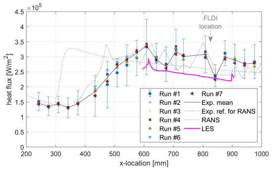
Figure 1.
Surface heat flux density distributions along the model for all seven shock tunnel runs. For clarity, the experimental standard deviations are suppressed for all but one run, and mean values across all runs are shown with a black solid line. The x coordinate is measured along the axis of the cone. Additionally shown are the distribution obtained in the LES used in the present work; the laminar and turbulent distributions in the precursor RANS simulation; and a previous experimental distribution obtained in HEG [54], which was used to define the boundary layer trip location in the RANS simulation.
Additional instrumentation pertinent to the analyses in this work includes a Z-type high-speed schlieren and a quad-foci Focused Laser Differential Interferometer (FLDI).
The schlieren system uses a Phantom v2012 camera and a Cavilux 640 nm laser source, with the knife edge oriented parallel to the surface of the cone. The images are acquired with a sampling rate of 57 kHz, which provides more than 100 frames within the shock tunnel steady-state time. The visualization area is approximately mm (streamwise × wall-normal) centered around the FLDI probing location, with a spatial resolution of approximately 24 pixels/mm.
The schlieren images are primarily used to estimate the boundary layer thickness in each run. This is performed by noting that the location of the maximum curvature of the wall-normal density distribution presents some proximity to that of of the velocity magnitude. High-speed conical laminar boundary layers on a cold wall under different HEG free stream conditions have been computed using the TAU code in past works [55,56]. Analyses of these computations have revealed that the locations of maximum curvature in density and of the velocity magnitude are within of each other. It will be seen in the computational results in Section 3 of the present work that this relationship is degraded in the turbulent boundary layer, with a difference of around . This value gives rise to measurement uncertainty, which should not be neglected, and it is therefore taken into account when analyzing the present results. It will be shown in Section 3.1 that the obtained boundary layer thickness estimates are still accurate enough for the purposes of this work.
Schlieren is used to estimate the boundary layer thickness as follows. The schlieren knife edge parallel to the model surface yields illumination proportional to the first derivative of the flowfield density along the wall-normal direction. Hence, the differences in pixel intensity along this same direction are representative of the second derivative of density, and the maximum curvature is a peak in these values. A reference schlieren flow topology image is obtained in each run as the average of all frames within the experimental steady-state time. For every column in the image (wall-normal direction), a vector of pixel intensity differences is obtained. The new image containing the distribution of the wall-normal differences in pixel intensity is then smoothed with a moving average of 200 pixels across the columns (streamwise direction). In this final image, the peak value along each column is marked as an approximation of the local boundary layer thickness. Finally, a linear regression is found using least squares considering all the points obtained across the full schlieren field of view. The boundary layer thickness at the probing location is calculated by evaluating the linear fit.
The estimates of the boundary layer thickness will be used in Section 3 and Section 4 to non-dimensionalize the FLDI probing positions in both the experimental and computational cases. Table 2 shows the boundary layer thickness obtained in each run in this work using the schlieren method above, together with the relative positions of the FLDI probes, to be detailed next.
Table 2.
Measured boundary layer thickness (approximate of ) and relative wall-normal positions of FLDI probes in each shock tunnel run.
The experimental FLDI setup employed in this work is a quad-foci FLDI, with four independent probes in a arrangement along the perpendicular streamwise and wall-normal directions. The streamwise pairs are used to obtain convection velocity estimates. The wall-normal splitting allows measurements of velocity and frequency spectra at two distances from the model wall simultaneously in each shock tunnel run.
The main characteristics of the quad-foci FLDI are listed in Table 3, in which is the laser wavelength, is the maximum beam width at the field lenses and d is the distance between the field lenses and the focus of the system. The separation between the interferometric pairs is denoted by and measured by analyzing the response of the system to a weak lens, as described in [33,57]. The separation between the independent FLDI probes in the streamwise direction, , is measured using the weak blast wave approach described in [58]. Finally, the separation between independent FLDI probes in the wall-normal direction, , is measured by means of direct imaging using the schlieren camera with a semi-transparent stopper at the focus of the FLDI.
Table 3.
Quad-foci FLDI setup information.
In order to allow simultaneous schlieren measurements in every run, the FLDI is used with an angle of with respect to the spanwise direction. This angle is considered when calculating the convection velocities. Nonetheless, the yaw represents a maximum streamwise difference of only mm between the right and left edges of the intersection between the FLDI axis and boundary layer under the conditions investigated in this work. Therefore, the angle will be disregarded in the interpretation of the frequency spectra in Section 4.
The splitting and recombination of beams for interferometry is obtained using a pair of Sanderson prisms [59], which is calibrated using the lens approach detailed in [33,57]. The Sanderson prism is oriented such as to split the interferometric pair in the streamwise direction. The selected interferometry distance seen in Table 3 is chosen so as to maximize the frequency bandwidth of the instrument, while still presenting a sufficient signal-to-noise ratio, based on previous HEG tests under similar conditions. The Nyquist frequency of the FLDI in the flowfield conditions investigated in this work is estimated as approximately 10 MHz.
The FLDI laser source is an Oxxius LCX-532S DPSS. The beam intensity is detected using a Thorlabs DET36A2 photodetector of nominal bandwidth 25 MHz. The photodetectors are connected with termination to an SRS SR445A DC-350 MHz preamplifier with amplification. The resulting signals are recorded on an AMOtronics transient recorder with DC coupling and a 100 MHz sampling rate. Conversion of the recorded voltage into the FLDI phase difference is performed following [60]. Prior to each shock tunnel run, the FLDI is adjusted to half the maximum output value, for optimal sensitivity.
The duplication of the FLDI probe in the streamwise direction is achieved using a Wollaston prism, as detailed in [58]. In the wall-normal direction, a second pair is obtained using the combination of a non-polarizing beamsplitter cube and a convergent lens of focal distance 400 mm near the laser source, as shown in Figure 2. A half-waveplate is used before the streamwise splitting to adjust the beams to similar power levels, such that all instruments present similar signal-to-noise ratios. The optical setup is such that the two FLDI probes that are closer to the model wall are slightly more powerful than the other two, but the powers of each streamwise pair of probes are identical.
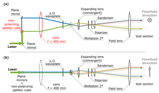
Figure 2.
Emitting side schematic of quad-foci FLDI with parallel beams in the probing region. Optical components responsible for the wall-normal system duplication are highlighted in red. Beam colors denote the center lines of independent FLDI probes (beam splitting for interferometry at the Sanderson prism not shown, for clarity). Parallel lines represented in close proximity to one another are overlapped in reality. Optical components that do not affect the beam paths in each view are represented using dashed lines. (a) Side view. (b) Top view.
The attention given in [58] to the production of parallel FLDI probes aiming at reliable convection velocity correlations is retained here. Therefore, the additions illustrated in Figure 2 are conceived such that all beams cross the center axis of the instrument at the focal distance of the field lens, where the Sanderson prism is located.
In all shock tunnel runs, the FLDI setup is positioned 825 mm downstream of the cone tip, measured along its axis. As highlighted in Figure 1, this location is approximately 200 mm downstream of the boundary layer transition region. This distance is chosen such that a turbulent boundary layer with well-developed features is probed.
In the wall-normal direction, the FLDI position is varied between runs, to compose a broad picture of the spectra and convection velocity distributions. The locations are listed in Table 2, comprising 5 stations fully inside the boundary layer, 4 stations between one and two times the boundary layer thickness and another 5 above this. Measurement of the wall-normal locations is performed by imaging a semi-transparent stopper at the focus of the FLDI with the schlieren camera, using additional lenses for improved resolution and a calibration target to provide a dimensional reference. The associated level of uncertainty (see Table 2), while not negligible, is considered tolerable when using the measured quantities as approximate wall-normal probing locations.
Frequency spectra from the FLDI measurements are calculated using Welch’s method with segments of points and overlap, on a 2 ms time window during steady state. The velocity estimates are obtained through cross-correlation between the streamwise-separated pairs of FLDI probes, using the same 2 ms time window, but divided into 20 segments of ms each with no overlap. This is done so that small fluctuations within the steady state are detectable, and the experimental uncertainty may be calculated.
2.2. Computational Tools
2.2.1. LES Solver
In the LES, Favre-filtered Navier–Stokes equations are solved via a six-order compact finite difference code originally developed by [61] and now under continued development at Purdue. The Quasi-Spectral Viscosity (QSV) approach [62] is used for turbulence closure. The time integration is carried out via a four-stage third-order strong stability preserving (SSP) Runge–Kutta scheme [63]. To ensure stability, the conservative variables are filtered using the sixth-order compact filter described by [64], with a filter coefficient of .
Only the turbulent region under the shock is simulated in the present LES. The computational domain, illustrated in Figure 3, extends from mm, with x measured along the cone wall. The azimuthal extent of the domain is 18 degrees. The domain height is 29 mm at the inlet and 44 mm at the outlet. The number of grid points is . Mean profiles at the inlet are given by a RANS simulation with the Spalart–Allmaras (SA) model [65]. The transition location for the RANS calculation is chosen by matching the experimentally observed beginning of the transition process. The heat flux profile of the RANS calculation shown in Figure 1 is different from experimental data around mm because the SA model does not reproduce the intermittency of the transition process. However, the magnitudes agree well with the experiment in the turbulent region. At the wall, an isothermal and a no-slip boundary condition are imposed with a wall temperature of 300 K. The flow properties at the upper boundary are analytically derived via the Taylor–Maccoll inviscid solution [66]. To generate realistic inflow turbulence, turbulent fluctuations are extracted at mm and imposed at the inflow by a rescaling method [67]. The recovery length, investigated in [68], has been found to be sufficiently short so as not to affect the region where cFLDI is carried out. At the outlet, a homogeneous Neumann condition is imposed for all flow quantities. In addition, sponge layers are used at the inlet, outlet and upper boundaries. The lengths of the sponge layers at the inlet and outlet are 3% of the total computational domain extent in the streamwise direction. At the upper boundary, it is 5% of the wall-normal extent.
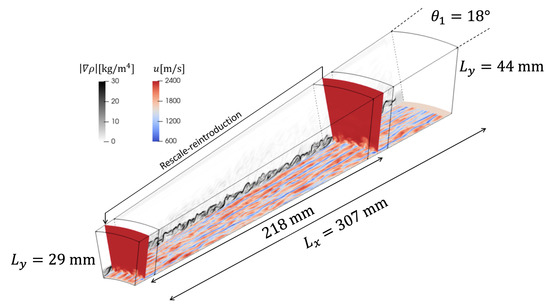
Figure 3.
Schematic of the present QSV-LES of a hypersonic boundary layer over a cone with rescaling. Streamwise velocity contours are shown in wall-parallel direction and cross-flow planes show streamwise velocity fields; magnitude of the flow density gradient is shown in a side plane.
2.2.2. Computational FLDI
The direct comparisons between experimental and numerical results in Section 4 will be performed using the FLDI output of phase difference, . The means to obtain this quantity on the LES is through computational FLDI (cFLDI). This algorithm is based on the ray-tracing model presented in [44], with further improvements detailed in [48]. A detailed description of the cFLDI algorithm used in the present work is presented in [49]. That work also validates the implemented cFLDI, using measurements on the flowfield generated by a weak blast wave. A summarized overview is presented next, for clarity.
The cFLDI algorithm simulates the behavior of light rays crossing a transparent volume containing density gradients. Variations in local density cause changes in the refraction index of the medium, which is perceived by the light rays as a change in the optical path. When two monochromatic and coherent light rays travel different optical paths, a phase difference between them is produced [69]. This is the phenomenon by which FLDI extracts information from a given flowfield.
In the cFLDI, the two orthogonally polarized beams that compose one FLDI instrument are discretized into a finite number of rays. Each ray in one beam has a corresponding pair in the other. After crossing the full probing volume, every pair of rays will present a phase difference between them, caused by the slightly different density fields. This phase difference is
where is the laser light wavelength, K is the Gladstone–Dale constant ( m/kg for nm) and are the spatial paths traveled by the beams, parametrically described by .
When the light rays are recombined on the receiving side of the FLDI, the phase difference between them modulates the light intensity. The FLDI instrument is always configured such that the resulting intensity is a mean value plus a fluctuating component, which is modulated by , for maximum sensitivity. Finally, the light intensity detected by the FLDI instrument is a scalar value corresponding to the combination of all light rays, weighted by the beam intensity distribution across its area. The FLDI in this work uses circular beams with an approximately Gaussian intensity distribution. Therefore, rays are described using radial r and angular coordinates, and the beam intensity profile is given by . The tilde denotes normalized variables, such that the integral of over the full area of the beam is unity. The radial coordinate follows the normalization by the local beam radius suggested in [44], with containing of the beam energy.
The equivalent phase shift corresponding to the integrated light intensity detected by the FLDI is hence given by
with given by Equation (1).
Equation (2) provides a scalar value that is directly comparable to the experimental output of the FLDI instrument, minimally post-processed to convert the voltage into a phase difference.
In the ray-tracing approach described above, the mesh used in the cFLDI presents a particular shape as the number of nodes is fixed in the cross-section of the beam, and the area across which they are distributed assumes a minimum value at the focus of the system. As such, it becomes necessary to interpolate the numerical flowfield density values on the cFLDI nodes. Linear interpolation is performed in the LES rectangular coordinates to allow the use of fast algorithms. The LES system is defined such that the y planes run parallel to the cone wall, with the z-coordinate being the azimuthal angle, (not to be confused with the FLDI angular coordinate, ). In this reference system, FLDI draws a curved path, as shown in Figure 4.
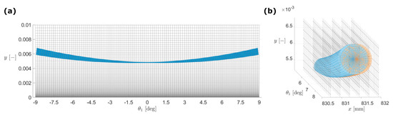
Figure 4.
Illustration of the computational meshes, in LES rectangular coordinates. (a) Front view, FLDI: blue dots, LES: gray lines. (b) Isometric view in the vicinity of the edge of the LES domain, FLDI: blue and orange lines, LES: gray lines and dots.
A mesh dependence analysis is performed before using cFLDI for comparisons between the numerical and experimental flowfields. The analysis is performed in a concise way, by selecting a probing height and a subset of the simulated time domain that are representative of the worst-case scenario. The strongest density fluctuations are observed in the upper portion of the boundary layer, between 3 and 6 mm from the model wall. Without loss of generality, the height of 4 mm and the time span of ms are chosen.
The cFLDI is discretized into uniformly distributed planes along its optical axis z. For the cross-section coordinates , the angular step is defined by the number of equally distributed points along the circumference . The approach suggested in [44] is adopted, by which is calculated as a function of such that each mesh cell conserves an aspect ratio close to unity.
Looking first at the discretization along the optical axis of the cFLDI, the LES mesh presents a m at the Cartesian center plane. Comparison of the cFLDI simulations using down to has shown negligible variation. Conservatively, a is kept, to ensure that any fluctuations resolved by the LES will be adequately interpolated in the cFLDI.
For the cross-section coordinates, several values for were evaluated. Figure 5 shows the obtained results. The cFLDI values are given in terms of density derivatives, which are obtained in a simple fashion using the known integration length provided by the LES domain to convert FLDI into a estimate. This is done so that a broad comparison may be drawn between the cFLDI output and a similar quantity that may be easily extracted from the LES, namely the integrated along a line of constant . This represents a straight horizontal line in Figure 4a, at the same height as the focus of the FLDI. Figure 5 shows that this simplified quantity and the cFLDI output are not the same, but have similarities. This will be further explored in Section 3.
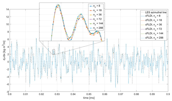
Figure 5.
Overview of the convergence analysis. The large plot shows the evaluated cFLDI cases, and the results from a simple line integral along the LES azimuthal direction. The detail shows the observed differences between the different cFLDI meshes.
Figure 5 shows that all the evaluated values of produce similar outputs. This is not surprising, given that the cFLDI mesh is naturally significantly finer than the LES one, particularly in the streamwise direction. Nonetheless, small differences can be seen in the detail. Using the finest evaluated mesh () as a reference, a zero-lag cross-correlation between its results and those from the remaining meshes is used to select the to be used in the analyses in this work. With (four times coarser), a cross-correlation value larger than is obtained. It is therefore selected as representing a converged mesh, each beam containing points . This mesh is illustrated in Figure 4b, together with the LES points.
3. Results
3.1. Experimental Data
The frequency spectra measured with FLDI in the experiments are compiled in Figure 6. The two gray lines correspond to the FLDI response shortly before flow arrival, as a reference of the noise floor of each streamwise pair of probes. The noise floor levels are slightly different due to the small power difference between the wall-normal pairs mentioned in Section 2.1. Flowfield measurements obtained across all shock tunnel runs are shown with different colors.
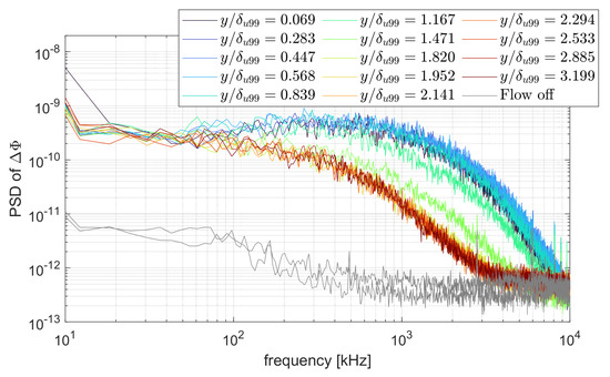
Figure 6.
Experimentally measured spectra of FLDI output . Data along a common wall-normal axis starting at the wall, with positions normalized by the thickness of the boundary layer measured in each respective run. The gray lines are flow-off references, obtained from the FLDI response before flow arrival.
Two well-defined groups of spectra are seen in the figure. First, measurements obtained above approximately two times the boundary layer thickness present little variation, collapsing together. This reiterates the repeatability of the multiple-run experiments and indicates an upper limit for the turbulent boundary layer influence. These results are in agreement with the hot-wire measurements of supersonic turbulent boundary layers in [12], where it is observed that fluctuations in the free stream do not become constant up to two boundary layer thicknesses away from the wall. Moreover, in the DNS investigation of a Mach 14 turbulent boundary layer in [18], the spectral distribution of pressure disturbances is very similar, between and times the boundary layer thickness. Additionally, in the cFLDI investigation of a Mach turbulent boundary layer DNS in [52], the RMS of the phase difference is observed to be constant only above times the boundary layer thickness.
The second group of spectra in Figure 6 concerns measurements fully inside the boundary layer. They present uniformly higher levels than the free stream, with the probe closest to the model wall () detecting marginally smaller amplitudes than the others. Although the coarse distribution of the measurement locations does not allow a precise observation, the region of maximum fluctuation in energy seems consistent with the of the boundary layer thickness verified in the hot-wire measurements of the Mach turbulent boundary layer in [28].
Below 100 kHz, all measurements register similar amplitudes. However, this is not to be interpreted as a flowfield characteristic. In this frequency range, the corresponding wavelengths are comparable to the maximum FLDI beam width in the test section, for the setup used in this work. Therefore, it is possible that contributions from the noisy shear layer surrounding the core flow are the cause of the overlap. This is to be further discussed in Section 4. Conversely, the higher end of the spectrum shows that the FLDI is capable of detecting disturbances with magnitudes above the noise floor, up to nearly 10 MHz. This is both a testament to the capability of the technique and an indication of the scales of energy-carrying density disturbances. At approximately 2 km/s, 10 MHz corresponds to a disturbance wavelength of m.
In the simplified case of neglecting the FLDI wavenumber-dependent sensitivity, the straightforward conversion of the FLDI phase differences into arbitrary units of density is possible. In this simplification, the phase differences are proportional to the density differences (or, in the limit, its derivative ). Therefore, the spectra of phase differences and density are related as [70]. Caveats of this approach will be presented with the discussion in the next section. The results of this simplified conversion using deconvolution are presented in Figure 7, together with lines representing reference power slopes. The density power spectra from Figure 7a are repeated in Figure 7b with the compensation of power to facilitate the visualization of the slopes. In Figure 7b, the rise in the free stream spectra starting at 3 MHz corresponds to the effect of the power compensation on the noise floor and should be ignored.
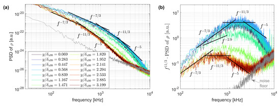
Figure 7.
Spectra of density, calculated using deconvolution from experimental FLDI measurements. Data along a common wall-normal axis starting at the wall, with positions normalized by the thickness of the boundary layer measured in each respective run. (a) Spectra. (b) Spectra compensated for slope.
The convection velocity measurements obtained from the cross-correlation of signals from the FLDI streamwise pairs are shown in Figure 8. Prior to cross-correlation, the FLDI signals are high-pass-filtered as shown in the legend. This will be further discussed in Section 4.1. Estimated uncertainties of the probing location are represented with vertical bars. They take into account both uncertainties pertaining to the measurement of the location of the FLDI probes with respect to the model wall and the uncertainty of the experimental measurement of the boundary layer thickness. The former are shown in Table 2, while the latter was estimated upon inspection of the LES results to be shown in Section 3.2. The resulting probing location uncertainties are within reasonable bounds to allow the verification of the overall behavior of the convection velocities across the boundary layer. The horizontal uncertainty bars represent the standard deviation of the 20 independent calculations on experimental data using ms time windows, as mentioned in Section 2.1. The measurements are verified to generally present little fluctuation within steady-state time, at less than inside the boundary layer and around in the free stream. The exception is the point at approximately times the measured boundary layer height, which presents a fluctuation. This is attributed to the intermittent passage of turbulent spots at this height, which could be observed in the schlieren images (not shown here).
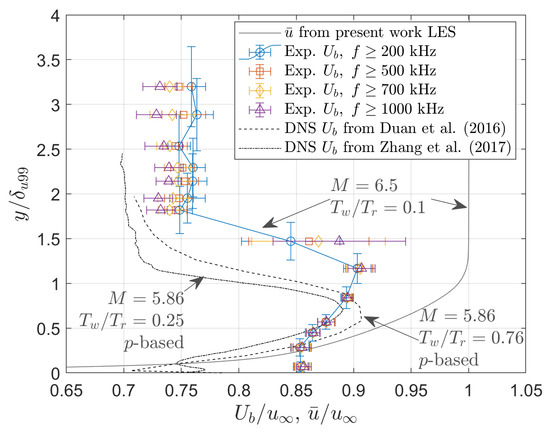
Figure 8.
Measured convection velocities across the hypersonic turbulent boundary layer. Measurement locations are indicated as distances to the model wall, normalized with the boundary layer thickness in each run. Uncertainty bars of measurement locations combine the uncertainties of position and boundary layer thickness measurements, shown for a single dataset for clarity. Velocities are normalized with the nominal flowfield velocity at the edge of the conical boundary layer. The mean velocity profile from the LES in the present work is shown as a reference. Experimental measurements based on density disturbances, high-pass-filtered over given frequencies. DNS data from [4,19] based on pressure disturbances on a flat plate with lower free stream Mach number are plotted for comparison.
The convection velocities are verified to be larger than the mean velocity close to the wall and smaller everywhere else. This is in agreement with the convection velocities in a Mach turbulent boundary layer presented in [28], in which the limiting height for this inversion was measured to be approximately of the boundary layer thickness. Moreover, in [28], the maximum convection velocities were approximately , similar to the results presented here, although, near the wall, the measured values were as low as . This discrepancy may be caused by the combination of two factors. First, the wall-to-recovery temperature ratio influences the convection velocity magnitudes near the wall, as seen in the velocity distributions from [4,19] plotted in Figure 8. In [28], this ratio is approximately . Second, it is possible that the integrating characteristic of the FLDI, to be further explored in Section 4, may bias the results very close to the model wall.
The velocity results shown in Figure 8 allow an estimation of the convection velocity of the density fluctuations in the free stream above the conical boundary layer. The average of these measurements in the case of the lowest high-pass frequency (200 kHz) is plotted in Figure 9 against the bulk velocity of pressure fluctuations available in the literature. In the figure, , with denoting the speed of sound in free stream conditions. The region below the line where pertains to disturbances convecting supersonically with respect to the free stream. The convection velocity measured in the present work, which falls within such a region, together with previous investigations, offers further evidence of the dominance of ‘Mach-wave-type’ acoustic radiation in the supersonic free stream [4,9,12,71].
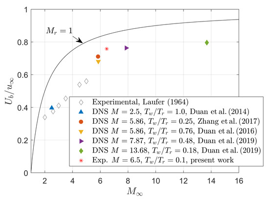
Figure 9.
Comparison of free stream convection velocities for a wide range of Mach numbers. Literature data refer to convection velocity of pressure disturbances, from experiments [12] and DNS [4,9,19,21].
3.2. LES Data
The time-resolved numerical solution was simulated for a total flowfield time of ms. In the conditions studied in this work, the rescaling–recycling flowthrough time is approximately ms. The mean boundary layer profiles are observed to undergo significant changes during the first cycles of rescaling–recycling. The steady-state time of the turbulent boundary layer is assessed by analyzing the wall shear stress over time, shown in Figure 10. A smoothed signal is shown on top of the raw data, to facilitate qualitative observations. The low-frequency, high-amplitude variations until approximately ms are evidence of the settling process. Conservatively, the time range below ms, marked with a dashed vertical line in the figure, is considered to be a transient settling time and is therefore discarded from the present study. The remaining simulated time, which comprises a total of 1 ms within ms, is detailed and analyzed next.
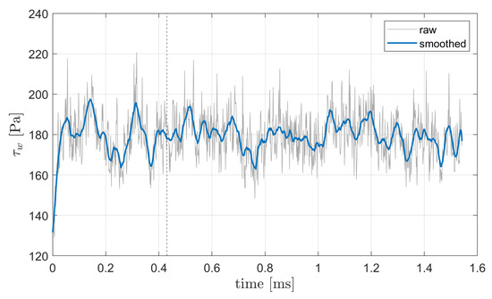
Figure 10.
LES wall shear stress over time. Raw and smoothed data are shown. The vertical dashed line at ms marks the beginning of the time range considered for analysis in the present study.
An illustration of the computational flowfield is shown in Figure 11, with a slice of time-varying density contours as they travel across a reference location. The slice has a constant wall-normal distance inside the boundary layer and a fixed streamwise position, with the azimuthal direction represented in the figure’s y-axis and time along the x-axis. A subset of the total time is shown, for clarity. This representation illustrates how the flowfield is perceived by an observer at a fixed position, such as the FLDI.
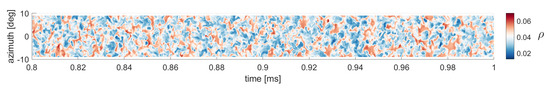
Figure 11.
LES time-resolved contours of density on a slice of constant wall-normal coordinate mm, with the LES azimuthal direction along the y-axis and time along the x-axis. A subset of the computational steady-state time is shown.
Figure 12 shows the LES mean distributions of streamwise velocity, density, pressure and temperature, averaged over both time and the azimuthal coordinate. The boundary layer thickness based on of the free stream velocity is annotated, as well as the location where the second difference in density is the maximum. As mentioned in Section 2.1, the latter is the quantity used to estimate the experimental boundary layer thickness from schlieren observations. Figure 12 shows that there is a difference between this and the true of approximately . This mismatch between the two quantities is considered when estimating uncertainties for the experimental measurements shown in Section 3.1.
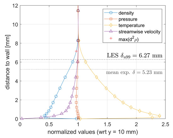
Figure 12.
Mean boundary layer profiles from LES. Values correspond to azimuthal averages, normalized by their values at mm. The boundary layer thickness corresponding to of the streamwise velocity magnitude is annotated. The location of the maximum second difference in density is highlighted with a “+” sign. The mean value of the experimentally measured boundary layer thicknesses is also represented for reference.
Nonetheless, when comparing the boundary layer thickness in the LES (Figure 12) and experiments (Table 2), a difference of nearly is observed. Despite this difference, the numerical boundary layer is obtained such that turbulence is fully developed and the heat flux magnitude is comparable to the experimental data. Therefore, when comparing experiments and computations in Section 4, the wall-normal coordinate is normalized by the boundary layer thickness in each case.
The frequency spectra of the azimuthally averaged density at the same relative positions as the experimental FLDI probes are compiled in Figure 13. To calculate the spectra, the time-resolved LES flowfield data are first averaged along the azimuthal direction. Then, the time-varying density values at a given distance from the wall are extracted and the spectral estimate is computed. The time-resolved azimuthal average of density represents the simplest approximation of the FLDI. Differences may be observed between these spectra and the corresponding experimental data in Figure 7. In the low-frequency range up to approximately 100 kHz, the experimental data follow power, while the LES data do not, starting to present this slope for larger frequencies only. Furthermore, the LES boundary layer data roll off from the power slope shortly above 1 MHz, while the experimental counterparts seem to follow this slope until at least MHz. These differences will be analyzed in Section 4.
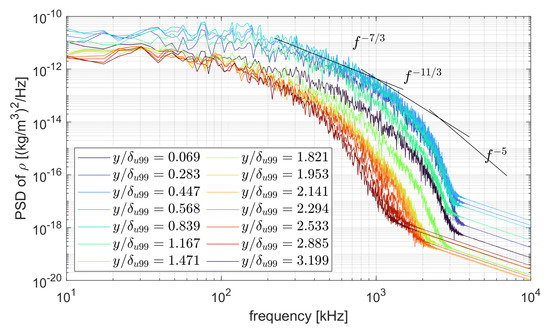
Figure 13.
Power spectral distribution of azimuthally averaged LES density, at wall-normal locations corresponding to the experimental probes.
Since the FLDI outputs a spatial differential measurement, the spectra of the first differences in density along the streamwise direction are plotted in Figure 14. This is a more directly comparable quantity to FLDI measurements. The differential density is extracted from the LES flowfield using values from adjacent grid planes in the streamwise direction.
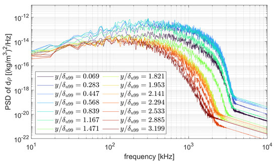
Figure 14.
Power spectral distribution of the first spatial differences along the streamwise direction of azimuthally averaged LES density, at wall-normal locations corresponding to the experimental probes.
Similarities to the experimental results previously shown in Figure 6 can be seen, such as the increased magnitudes when inside the boundary layer and the two distinct groups of spectra. Nonetheless, similarly to the density spectra, differences can be observed in terms of roll-off, especially for frequencies above 1 MHz. This is both an effect of the streamwise resolution of the numerical grid, which limits the wavelength that can be resolved, and the artificial damping necessary to provide stability to the numerical solution. The identification of such constraints is the main goal of Section 4.3.
Convection velocities are calculated on the numerical flowfield for comparison with the experiments. Time-resolved data at the same relative positions as the experiments are extracted and cross-correlated to determine the convection velocities. The flowfield variables are averaged along the LES azimuthal direction, for better comparison with FLDI measurements. Cross-correlation is performed with signals from streamwise planes separated by approximately the same distance of the experimental FLDI velocimetry pair. Similar to the experimental case, velocity measurements are obtained in subsets of ms and combined into an average value. The results of convection velocities obtained from density and pressure signals are shown in Figure 15. The high-pass filtering used in the experimental case is also repeated here. When filtering above 1 MHz outside the boundary layer, the resulting signal retains little of the simulated flowfield (see the spectral amplitudes in Figure 13). The velocity measurements in such cases are therefore discarded.
Figure 15.
Convection velocities across the LES hypersonic turbulent boundary layer, based on (a) density and (b) pressure disturbances. Annotations shown in (a) are also valid for (b). Wall-normal distances along the x-axis are normalized by the LES boundary layer thickness . Velocities in the y-axis are normalized with the flowfield velocity at . The mean velocity profile is shown as a reference. DNS data from [4,19] based on pressure disturbances on a flat plate with lower free stream Mach number are plotted for comparison.
3.3. Computational FLDI
Computational FLDI (cFLDI) was simulated on the LES flowfield, at the normalized positions corresponding to the experimental probes. The spectral distributions of the cFLDI probes are shown in Figure 16.
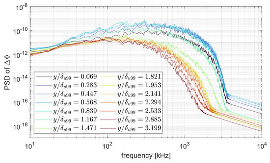
Figure 16.
Spectra of cFLDI output , at wall-normal locations on the LES flowfield corresponding to the experimental probes.
In this figure, the y-axis is set to display the same number of decades as Figure 14. Despite the different dimensional units of the time series, namely kg/m in Figure 14 and radians in Figure 16, it is possible to notice strong similarities in the spectral distributions. This will be further explored in Section 4.5.
4. Discussion
4.1. Velocity Measurements
Figure 8 shows that the distributions of the convection velocities of density disturbances are overall similar to the DNS results of [4,19], with a larger velocity in the boundary layer and a rather significant drop in the free stream. The maxima and free stream values are also close.
Despite the agreement in shape, however, the experimental results show evident displacement towards the free stream. This may be an effect of the different wall-to-recovery temperatures. There is also a difference in the velocity distribution very close to the wall. In addition to the different wall temperature, the finite FLDI-sensitive length and probing along a secant line through the boundary layer might cause this effect. In order to probe very closely to the wall, the FLDI must cross through the entire boundary layer. In the present setup, the length of the intersection between the FLDI and the boundary layer is approximately 60 mm. As demonstrated in Figure 17, the spatial filter effect of the present FLDI within this distance is small for frequencies as high as 1 MHz. It is therefore subject to accumulated contributions from regions of strong density fluctuation in the vicinity of the focal plane. This is further indicated by the distribution of the convection velocities in the LES results in Figure 15, which do not share this issue and follow the results in [4] more closely near the wall.
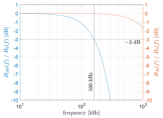
Figure 17.
Loss of FLDI transfer function due to spatial filtering, evaluated for multiple frequencies at two distances from the center plane: 250 mm (left y-axis), representative of the nozzle shear layer, and 30 mm (right y-axis), representative of the edge of the conical boundary layer.
The velocity distributions shown in Figure 8 evidence an overall distinction between the convection velocity of the density disturbances and the local mean flowfield velocity. The departure is greater in the free stream than in the boundary layer, but the boundary layer effect is still noticeable, at least up to times of its thickness. Furthermore, disturbances of different sizes, which correspond to different frequency bounds in Figure 8, convect with similar velocities in the boundary layer. In the free stream, smaller disturbances (higher frequencies) convect slightly slower than larger ones (lower frequencies). However, the influence of the boundary layer extends further into the free stream for smaller disturbances than for larger ones.
The numerical results in Figure 15 show that the convection velocities based on pressure fluctuations in the boundary layer are comparable with the experimental measurements. This also holds for large disturbances in the free stream for both density and pressure, within a small difference. Conversely, the boundary layer density disturbances in the LES convect at larger velocities than the experimental and LES pressure-based velocities. Additionally, smaller disturbances of both pressure and density in the LES present increasingly larger convection velocities farther away from the model wall, unlike the experimental measurements. These discrepancies require additional analyses of the numerical solution, which are beyond the scope of the present work.
The addition of this work’s experimental mean free stream convection velocity to the dataset in Figure 9 allows the verification that the velocity measurements based on density fluctuations yield comparable values to existing pressure-based ones. When considering the extrapolation of the literature points, a slight upward offset of the present measurement can be seen. This agrees with the trend observed in the two similar DNS points of , in which a colder wall corresponds to a larger eddy convection velocity.
The observed agreement between the convection velocities of pressure and density disturbances is an expected result, since the free stream flowfield can be regarded as isentropic. Nonetheless, contrary to other methods, such as DNS or intrusive experimental devices that measure localized quantities, the FLDI is an integrating instrument. Therefore, the verification that the FLDI measurements are similar to other available data despite this fundamental difference is an important result. It indicates that the existing database of bulk velocity information may be complemented with multi-foci FLDI measurements.
4.2. Spectra of Density Fluctuations
The spectra of density fluctuations shown in Figure 7 allow the observation of the energy cascade of the density disturbances. In an environment dominated by acoustic disturbances, the flowfield is isentropic and thus pressure and density fluctuations are correlated by a constant (square of the sound speed). Therefore, it makes sense to analyze the energy cascade detected by the FLDI in light of the expected behavior of pressure, as a first approximation. The power laws for pressure spectra are represented together with the experimental density data in the figure, for reference.
In [72], power laws are derived for the spectral distribution of pressure fluctuations in a shear flow. Interactions of the turbulence–turbulence type are found therein to follow a decay, while turbulence–mean shear interactions decay as (second moment) and (third moment). The two latter decays are experimentally observed in the density spectra of a Mach 2 shear layer in [8] and associated with isotropic and anisotropic turbulence, respectively. Nevertheless, in the mentioned work, anisotropic turbulence was observed at low-to-moderate wavenumbers, with power laws measured between and , while isotropic turbulence was found at high wavenumbers. The decay has also been experimentally observed in the Mach free stream pressure fluctuation measurements of [73].
The turbulence–turbulence decay is analogous to Kolmogorov’s power law for velocity [30] and relates to acoustic disturbances (eddy Mach waves). It has been experimentally observed in the farfield of a Mach turbulent boundary layer in [12]. More recent DNS studies have also detected the slope at the wall of a transonic turbulent boundary layer with an adverse pressure gradient in [74] and in the Mach free stream above a turbulent boundary layer in [9]. It must be noted, however, that this slope was not present in the DNS investigation of a Mach turbulent boundary layer in [4]. A scaling value of power is mentioned in [4,74] and attributed to sources in the inner region of the turbulent boundary layer.
It is seen in Figure 7 that the experimental spectra of density fluctuations obtained in the present work follow the power laws to some extent. Both the free stream and the boundary layer have regions described by these scalings, albeit within different frequency ranges. A rather large region following the power slope is seen for both the boundary layer and free stream. This indicates a significant contribution of acoustic disturbances to the turbulent energy. It may be related to the noisy shock tunnel environment [75], which is dominated by acoustic disturbances, but only partially, as it is also present in the LES spectra in Figure 13. Interestingly, the power slope is well defined in measurements at distances more than two times the thickness of the boundary layer. Since this behavior is linked to boundary layer sources, this could be an indication of energy emission into the free stream. However, given that the source of the slope is found to the sublayer region below [4], more intricate phenomena would then be responsible for allowing this to reach the free stream, the investigation of which is beyond the scope of this work.
Although these observations are useful to provide insight into the mechanisms governing the energy cascade in hypersonic flowfields, they must be interpreted with caution. As mentioned in Section 3.1, the spectral distribution of densities was obtained by assuming direct proportionality between the FLDI phase differences and the flowfield density fluctuations. This hypothesis neglects the wavenumber-dependent sensitivity length of the FLDI. The simplification is reasonable for low frequencies up to a certain threshold, as it can be seen in Figure 13 that the density spectra directly calculated from the numerical flowfield also agree with the power in an intermediate range of frequencies.
However, in order to correctly convert the high end of the FLDI spectrum, more sophisticated approaches are needed. Furthermore, the threshold to use the simplified approach of merely deconvolving on the FLDI data is not easily defined. The following sections discuss computational FLDI as an alternative solution for direct comparison between experimental and numerical results. Once the comparison is established, it becomes possible to take advantage of the insight given by the numerical investigation without the need to directly address the complexity of the experimental measurement instrument.
4.3. Constraints for Experimental and Numerical Direct Spectral Comparison
For direct comparisons between computational and experimental FLDI results, it is important to consider the limitations pertinent to each environment.
In the experiments, the FLDI instrument must run through a noisy shear layer that surrounds the core flowfield. The wavenumber-dependent sensitivity length of the instrument is well explored in [33]. It is such that high-frequency content is only detected near the center plane, but the lower end of the spectrum is detected along the entire optical axis. Therefore, the shear layer imposes a lower limit on the useful frequency response of the FLDI, below which the measurements are dominated by shear layer content [11,52]. However, the limit is not a well-defined value, as the FLDI response to a disturbance of a given wavenumber rolls off continuously away from the center plane.
A methodology to assess the lower bound of the FLDI bandwidth in the presence of strong disturbances surrounding the flowfield is presented in [76]. The method is based on a ratio of sensitivity functions between the volume of interest and the noisy region, and it uses the transfer functions of the FLDI instrument and assumptions on the average amplitudes of disturbances across the probed volume. This approach has been applied to a test case of free stream measurements through a nozzle shear layer in [11]. In the present work, a simplified approach is chosen, aiming at a plane-by-plane analysis, as will be shown. This is a less conservative approach than the more complex method of [76], but is preferred in this work for two main reasons. First, it does not require explicit assumptions on the spatial distribution of disturbance magnitudes. Second, for the present case, at the same time that the direct contribution of the shear layer to the FLDI signal is constrained to the edges of the flowfield volume, the total width of the shear layers is comparable to the length of the intersection between the FLDI and the turbulent boundary layer. This means that the contribution of a signal either in the shear layer or in the boundary layer will be similar in terms of spatial integration. Nonetheless, the FLDI filtering effect away from the focus will cause the damping of the amplitudes at the location of the shear layer. This damping is evaluated using transfer functions as follows.
The FLDI transfer function is defined as the ratio between the spatial derivative measured by the instrument and a true spatial derivative of the same disturbance field. As explored by many authors [33,44,45,76], a useful reference disturbance field is a single-frequency sinusoidal wave of infinitesimal thickness. The transfer function representing the FLDI spatial filtering in this case is
where w is the local FLDI beam radius and k is the wavenumber of the sinusoidal wave, which relates to frequency f and convection velocity as . The use of this formulation to evaluate the FLDI wavenumber-dependent sensitivity length has been experimentally validated in [45], through analyses of multiple ultrasonic wavefronts of well-defined frequencies.
In the shock tunnel experiments reported here, the core flowfield presents a radius of approximately 250 mm [53]. Equation (3) is therefore used to evaluate the FLDI transfer function magnitudes at this location, denoted for simplicity as , for a wide range of wavenumbers. Corresponding reference magnitudes at the center plane, denoted , are also evaluated. The comparison between them provides a wavenumber-resolved loss parameter, shown in Figure 17. For a more straightforward interpretation, the figure displays the results plotted against frequencies obtained from wavenumbers using the measured free stream convection velocity of approximately , as shown in Figure 8.
Without losing generality, a loss of dB is defined as a reference bound. This corresponds to a half power decay, before which the signal amplitudes detected in the shear layer are expected to be significant enough to bias the measurements from the core flowfield. Figure 17 shows that at 250 mm from the center plane, the FLDI in the present work presents a dB loss at kHz. The experimental spectra below this frequency value are hence discarded. It should be noted that despite the simplifications contained in this approach, this value is in agreement with the experimental spectra shown in Figure 6, which show separate amplitudes between the boundary layer and free stream in the vicinity of this frequency. If the contribution of the shear layer was not sufficiently damped, an overlap of the spectral amplitudes would be expected, such as in the region below 100 kHz in the figure.
An additional line is plotted in Figure 17 using the right y-axis for the transfer function magnitudes at a distance of 30 mm from the focal plane, corresponding to the boundary layer intersection mentioned in Section 4.1. It is verified that, in this case, the transfer function value remains close to the best focus reference across all evaluated frequencies, which represents the weak spatial filter effect in this analysis.
Additional limitations must be considered at the opposite end of the spectrum, towards extremely high frequencies. First, the experimental measurement capabilities are limited by the FLDI beam separation distance . Wavelengths smaller than twice the separation cannot be resolved. In the present case, m, which corresponds to 10 MHz in the free stream and 12 MHz in the boundary layer, using the velocity information in Figure 8. These are constraints of a spatial nature. The oversampling in the time domain, which, in the present work, is 100 MHz (see Section 2.1), favors the proper detection of amplitudes in addition to frequencies. It is important to highlight that a compromise must be made between and the signal-to-noise ratio, since the differences between two points will be smaller as the distance between them is reduced. In this regard, Figure 6 shows that the FLDI in the present work was able to optimize this trade-off.
A second high-frequency constraint relates once more to the wavenumber-dependent sensitivity length of the FLDI. At this edge of the spectrum, it is possible that the same spatial filtering that allows the instrument to see through the shear layer starts damping information within the scope of the investigation. This is especially the case for the free stream spectra in the present work. The conical flowfield contributions to the FLDI signal are expected to be approximately equal throughout the probing volume, or at least within the boundaries of the conical shock (notwithstanding, the circular symmetry of the flowfield surrounding the conical model must be properly considered when probing along a straight-line FLDI, as seen in [49]). With such an extensive probing volume, the influence of the varying sensitive length is expected to cause significant amplitude differences across the frequency spectrum. The resulting FLDI signal accumulates contributions from lower-frequency disturbances across the full probing length, while higher frequencies contribute only along a limited portion of it. Such cases are the main motivation to use the transfer function approaches from [33,46,47]. However, these functions must be obtained while respecting the flowfield characteristics, and the derivation of a transfer function for conical flowfields is beyond the scope of the present work.
Turning to the numerical flowfield, constraints for FLDI comparison concern the resolved frequency bandwidth and the limited spatial domain. The frequency bandwidth is determined by three factors: the temporal resolution of the LES; the spatial resolution of the grid; and the explicit spatial filtering required for the numerical stability of the compact finite difference scheme. In the present case, the temporal resolution of s is enough to provide reliable amplitudes up to at least 7 MHz, assuming a conservative oversampling of 10 times. The grid resolution is m, yielding a Nyquist limit of approximately 4 MHz, assuming a flowfield velocity of 2 km/s. The sixth-order compact filter dampens high-frequency phenomena starting with a weakened effect above 1 MHz and becoming progressively stronger at higher frequencies, due to its non-sharp spectral behavior. The effect is shown in Figure 13, Figure 14 and Figure 16. Representing the stricter high-frequency constraint in the present dataset, the upper bound of 1 MHz is chosen for the numerical and experimental comparisons in Section 4.4.
Lastly, the limited spatial domain of the LES may impose a constraint for experimental and numerical comparisons that relates yet again to the FLDI spatial filtering. If a numerical flowfield is obtained along the full FLDI probing length, then the spatial filtering of high frequencies is also present in the cFLDI simulation. In this case, direct comparisons between experimental and computational FLDI are valid without the need to correct the amplitudes in any way. If, on the other hand, the simulated flowfield corresponds to a section of the volume that contributes to the FLDI signal, the comparison is still possible, albeit with further considerations. One option is to correct for the FLDI spatial filtering in some way, as mentioned above. Alternatively, the comparisons must be restricted to frequencies above a certain value, similar to the shear layer analysis presented earlier in this section.
4.4. Direct Comparison between Experimental and Numerical Spectra
The conical boundary layer offers an advantage in the sense of the preceding observations. The amplitudes of the fluctuations inside the boundary layer are much larger than in the free stream. Furthermore, the FLDI crosses the conical boundary layer following a secant line close to its edge. Therefore, the volume largely contributing to the FLDI signal is much reduced. For example, when the FLDI is positioned at a height of , the length of intersection between the FLDI and the boundary layer is approximately 30 mm. This length has initially informed the definition of the size of the LES domain in this work, which presents a large enough azimuthal width to comprise the entirety of the intersection at this height. As a result, in the upper portion of the boundary layer, the full length of the intersection between the FLDI and the conical boundary layer is calculated.
This means that for a subset of the experimental and numerical data presented in Figure 6 and Figure 13, respectively, a direct comparison is allowed with minimum constraints. Figure 18 displays the comparison for three probing stations inside the boundary layer, namely and .
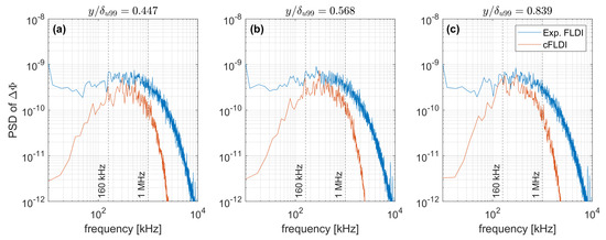
Figure 18.
Direct comparison between the spectra of phase differences from experimental FLDI and cFLDI calculated on the LES, for three different locations. (a) , (b) and (c) . The lower and upper frequency bounds for the comparison are shown as dashed lines.
These results show encouraging agreement between the experimental and numerical results within an intermediate range of frequencies. This range agrees to a certain extent with that obtained from the analyses in Section 4.3, namely 160 kHz MHz.
It is important to highlight the low-frequency bound of kHz determined in the previous section. Figure 18 confirms that indeed the experimental and numerical lines diverge significantly for frequencies below approximately this value. This is an indication that the lower frequencies in the experimental results have an origin other than the boundary layer. Therefore, it is paramount that a high-pass filter is used when employing FLDI for shock tunnel velocimetry, as exemplified in Figure 8. Otherwise, the signals being cross-correlated will most likely contain spurious low-frequency contributions, which have a strong impact on the cross-correlation operation and may thus bias the results.
Nonetheless, as mentioned before, the FLDI filter effect rolls off continuously, meaning that there is no unique means of finding a cut-off limit. Hence, there is an inevitable level of arbitrariness when choosing how to define a threshold. The dB loss with respect to the response at the focus was chosen in the present work, but alternative metrics have been previously used in the literature, such as folding in the RMS response [32] or the full-width half maximum (FWHM) of the transfer function [47]. This stresses the importance of having complementary methods of checking the calculated limit. In the present work, these are the simultaneous measurement of the free stream and boundary layer disturbances and the direct comparison to numerical results.
4.5. On the Simplified Comparison between Experimental FLDI and Numerical Solutions
As mentioned in Section 3, there is apparent similarity between the cFLDI spectra in Figure 16 and the LES spectra in Figure 14. This is an indication that the focusing effects of the FLDI are negligible.
An analysis similar to the one in Figure 17 was performed to evaluate the spatial filtering effect within the LES domain. At the edges of the boundary layer intersection previously mentioned, frequencies below MHz still retain over of the FLDI center plane sensitivity. In other words, the FLDI spatial filtering effect is very small in the boundary layer within the frequency bandwidth resolved by the LES.
In such cases, fluctuations in density and FLDI output are correlated in an almost direct manner, as a simplification of Equation (1):
where is the summation (line integral) of the density fluctuations along a line crossing the LES volume at any given time instant, and L is the length of this line.
Figure 19 shows the result of evaluating Equation (4) along a line of constant wall-normal coordinates in the LES rectangular system of coordinates, which is equivalent to a horizontal line in Figure 4a. It is denoted ‘cFLDI approximation’ and plotted together with experimental and computational FLDI at the same probing height, measured at the center plane.
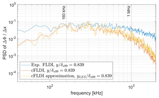
Figure 19.
Comparison between spectra of phase differences at a single probing location. The spectra are obtained from experimental FLDI, cFLDI on the LES solution and a simplified, approximate conversion directly on the LES. The lower and upper frequency bounds for the comparison are shown as dashed lines.
As expected from the previous observations, the results show strong similarities, despite the large complexity gap between the cFLDI algorithm and the straightforward estimation. Most importantly, there is similarity between the latter and the experimental data. This shows that useful comparisons might also be performed using a very simple formulation on the LES flowfield, in the absence of a complex cFLDI algorithm.
Evidently, the case presented here presents some facilitating properties, such as a very weak FLDI filtering effect within the volume of interest, low flowfield curvature and the computational simulation of the entire relevant volume. Nonetheless, the possibility of numerical and experimental comparison with such simplicity is encouraging.
5. Conclusions
This work has reported on the investigation of a turbulent boundary layer with cold walls at a free stream Mach number and unit Reynolds number m. Experimental shock tunnel data were analyzed in combination with a Large-Eddy Simulation (LES) under the same flowfield conditions to allow direct comparison. The main measurement technique was Focused Laser Differential Interferometry (FLDI), employed in a multi-foci arrangement with all probes parallel to each other for optimal signal cross-correlation.
The convection velocities of the density disturbances were experimentally measured using the cross-correlation of streamwise FLDI pairs along several locations inside the boundary layer and in the nearby free stream. Evidence of spurious low-frequency contributions likely coming from the nozzle shear layer highlighted the importance of high-pass filtering the FLDI signal before the cross-correlation operation. Results show the convection velocity to be highest slightly above the boundary layer edge at approximately times the free stream velocity. Farther away from the boundary layer edge, the convection velocity was verified to drop to approximately times that of the free stream, with larger disturbances propagating slightly faster than smaller ones. The magnitude of the measured convection velocity of the density disturbances is in agreement with the literature data on pressure disturbances in supersonic flows. An exception was observed when probing very close to the model wall, at approximately of the boundary layer thickness, due to the contribution of the upper layers of the conical boundary layer to the FLDI signal. An improvement in future works might be obtained by increasing the beam convergence of the FLDI setup, which will enhance its filtering ability away from the focal plane. In the LES, the convection velocities presented similar behavior when pressure disturbances were evaluated, but significant differences for density disturbances. This discrepancy requires further investigation, which was beyond the scope of the present work. Future work shall also investigate the LES flowfield beyond the data directly related to FLDI diagnostics, e.g., temperature–velocity relationship, strong Reynolds analogy, among others.
The experimental spectra of the density fluctuations across the turbulent boundary layer were evaluated and compared to power laws reported in the literature for pressure fluctuations. The FLDI data were able to evidence the presence of regions with identifiable power laws of , and . However, the upper limit of the frequency spectrum may have been biased by the FLDI frequency-dependent sensitive length, which was not compensated for in this work.
A framework to enable FLDI comparisons despite this complexity was explored by means of the use of computational FLDI (cFLDI) on the LES flowfield. Constraining conditions pertaining to both low and high ends of the frequency spectrum were detailed. The former was related to the noisy shear layer of the experimental flowfield and was calculated to be 160 kHz. The latter was around 10 MHz for the experimental FLDI and around 1 MHz for the computational solution. Furthermore, comparisons were performed in probing locations where the straight-line FLDI and the circular boundary layer within the LES domain presented significant intersection, as most of the flowfield disturbances were expected to be contained therein. Within these bounds, experimental and numerical direct comparisons yielded reasonable agreement. Encouraging agreement was also seen when a simple line integral of the computational data was analyzed in place of the complex cFLDI algorithm.
Overall, these observations present a positive scenario for future developments towards the understanding of high-speed turbulence, concerning experimental and numerical comparisons. In the absence of a complete model of cFLDI in groups focused on numerical investigations, useful data for spectral comparisons with experiments may be provided in a much simpler manner. At the same time, data provided by experimentalists can be used with minimal post-processing in numerical comparisons, as long as the necessary information for the determination of the constraining frequency bounds is also provided.
Author Contributions
Conceptualization, G.P.C., A.W., T.T. and C.S.; Data curation, G.P.C. and T.T.; Formal analysis, G.P.C.; Funding acquisition, A.W. and C.S.; Investigation, G.P.C., A.W. and T.T.; Methodology, G.P.C.; Project administration, G.P.C., A.W. and C.S.; Resources, A.W. and C.S.; Software, G.P.C. and T.T.; Supervision, A.W. and C.S.; Validation, G.P.C. and T.T.; Visualization, G.P.C.; Writing—original draft, G.P.C.; Writing—review and editing, A.W., T.T. and C.S. All authors have read and agreed to the published version of the manuscript.
Funding
This research received no external funding.
Data Availability Statement
The data that support the findings of this study are available from the corresponding author upon reasonable request.
Acknowledgments
The support given by Klaus Hannemann and Peter J. Klar is deeply appreciated. The authors also wish to acknowledge the assistance of Mariasole Laureti and the HEG team, particularly Ingo Schwendtke, Uwe Frenzel, Fabian Glasewald, Jan Martinez Schramm and Divek Surujhlal. The technical discussions with Victor C. B. Sousa and Emmanuel Gil Torres are also appreciated.
Conflicts of Interest
The authors declare no conflict of interest.
Abbreviations
The following abbreviations are used in this manuscript:
| CFD | Computational Fluid Dynamics |
| cFLDI | Computational Focused Laser Differential Interferometer |
| DNS | Direct Numerical Simulation |
| FLDI | Focused Laser Differential Interferometer |
| HEG | High-Enthalpy Shock Tunnel Göttingen |
| LES | Large-Eddy Simulation |
| RANS | Reynolds-Averaged Navier–Stokes |
| SA | Spalart–Allmaras |
| QSV | Quasi-Spectral Viscosity |
Appendix A
A complete set of flowfield parameters, aimed at allowing the flowfield investigated in the present paper to be reproduced, is given in this appendix.
In the experiments, the cone model is placed partly inside the nozzle. This is needed to allow the investigation of the fully developed turbulent boundary layer at mm, as seen in Section 2.1, while using the existing test section windows in HEG and avoiding any effects of the nozzle shear layer interacting with the model. Nevertheless, the tip of the model is positioned in a region of the nozzle where the flowfield surrounding it is already sufficiently developed.
Flowfield information is extracted from a RANS solution of the nozzle flow, calculated from experimental stagnation conditions that were measured in the present investigation. The extraction is performed along a line upstream of the shock wave produced by the cone model, as shown in Figure A1.

Figure A1.
Topology of the flowfield around the cone model partly inside the nozzle. The line along which spatially resolved properties are extracted is highlighted.
Figure A1.
Topology of the flowfield around the cone model partly inside the nozzle. The line along which spatially resolved properties are extracted is highlighted.

The flowfield properties are separated into two groups, depending on their variation along the extracted line. The properties displayed in Table A1 present fluctuations in the order of and are therefore assumed constant. In the table, refers to the mass fraction of species i, is the ratio of specific heats and R is the gas constant.
Table A1.
Flowfield properties that are constant along the extracted line from the RANS solution of the nozzle, calculated under experimentally observed stagnation conditions.
Table A1.
Flowfield properties that are constant along the extracted line from the RANS solution of the nozzle, calculated under experimentally observed stagnation conditions.
| [MPa] | [-] | [-] | [-] | [-] | [-] | R [J/(kg·K)] |
|---|---|---|---|---|---|---|
In Table A2, the properties showing non-negligible variation are listed with the spatial resolution. A total of 6 points are given for each property, uniformly distributed along the extracted line. When these points are used as references for a spline interpolation, the spatial distributions of the flowfield properties are reproduced with accuracy. The coordinate system has its origin at the tip of the cone model, as shown in Figure A1. The velocity components along the x and y axes are denoted u and v, respectively. Although u is nearly constant, it is included in Table A2 for completeness.
Table A2.
Spatially resolved flowfield properties, extracted along a line from the RANS solution of the nozzle, calculated under experimentally observed stagnation conditions.
Table A2.
Spatially resolved flowfield properties, extracted along a line from the RANS solution of the nozzle, calculated under experimentally observed stagnation conditions.
| x [m] | y [m] | u [m/s] | v [m/s] | p [Pa] | T [K] | M [-] | [kg/(m·s)] | [kg/m] |
|---|---|---|---|---|---|---|---|---|
References
- Ingenito, A.; Bruno, C. Physics and Regimes of Supersonic Combustion. AIAA J. 2010, 48, 515–525. [Google Scholar] [CrossRef]
- Roy, C.J.; Blottner, F.G. Review and assessment of turbulence models for hypersonic flows. Prog. Aerosp. Sci. 2006, 42, 469–530. [Google Scholar] [CrossRef]
- Pirozzoli, S.; Bernardini, M. Turbulence in supersonic boundary layers at moderate Reynolds number. J. Fluid Mech. 2011, 688, 120. [Google Scholar] [CrossRef]
- Duan, L.; Choudhari, M.M.; Zhang, C. Pressure fluctuations induced by a hypersonic turbulent boundary layer. J. Fluid Mech. 2016, 804, 578–607. [Google Scholar] [CrossRef] [PubMed]
- Zhang, C.; Duan, L.; Choudhari, M.M. Direct Numerical Simulation Database for Supersonic and Hypersonic Turbulent Boundary Layers. AIAA J. 2018, 56, 4297–4311. [Google Scholar] [CrossRef] [PubMed]
- Harvey, J.; Bergman, R.; Holden, M. An experimental study of hypersonic turbulence on a sharp cone. In Proceedings of the 20th Fluid Dynamics, Plasma Dynamics and Lasers Conference, Buffalo, NY, USA, 12–14 June 1989. [Google Scholar] [CrossRef]
- Yoder, D.; DeBonis, J.; Georgiadis, N. Modeling of turbulent free shear flows. Comput. Fluids 2015, 117, 212–232. [Google Scholar] [CrossRef]
- Papamoschou, D.; Robey, H.F. Optical technique for direct measurement of power spectra in compressible turbulence. Exp. Fluids 1994, 17, 10–15. [Google Scholar] [CrossRef]
- Duan, L.; Choudhari, M.M.; Wu, M. Numerical study of acoustic radiation due to a supersonic turbulent boundary layer. J. Fluid Mech. 2014, 746, 165–192. [Google Scholar] [CrossRef]
- Lawson, J.M.; Neet, M.C.; Hofferth, J.W.; Austin, J.M. Supersonic Freestream Density Fluctuations from Focused Laser Differential Interferometry and Pitot-Probe Measurements. AIAA J. 2022, 60, 5173–5186. [Google Scholar] [CrossRef]
- Gillespie, G.I.; Ceruzzi, A.P.; Laurence, S.J. A multi-point focused laser differential interferometer for characterizing freestream disturbances in hypersonic wind tunnels. Exp. Fluids 2022, 63, 180. [Google Scholar] [CrossRef]
- Laufer, J. Some Statistical Properties of the Pressure Field Radiated by a Turbulent Boundary Layer. Phys. Fluids 1964, 7, 1191. [Google Scholar] [CrossRef]
- Martin, M.P. Direct numerical simulation of hypersonic turbulent boundary layers. Part 1. Initialization and comparison with experiments. J. Fluid Mech. 2007, 570, 347–364. [Google Scholar] [CrossRef]
- Bernardini, M.; Pirozzoli, S. Wall pressure fluctuations beneath supersonic turbulent boundary layers. Phys. Fluids 2011, 23, 085102. [Google Scholar] [CrossRef]
- Lagha, M.; Kim, J.; Eldredge, J.D.; Zhong, X. Near-wall dynamics of compressible boundary layers. Phys. Fluids 2011, 23, 065109. [Google Scholar] [CrossRef]
- Duan, L.; Beekman, I.; Martin, M.P. Direct numerical simulation of hypersonic turbulent boundary layers. Part 3. Effect of Mach number. J. Fluid Mech. 2011, 672, 245–267. [Google Scholar] [CrossRef]
- Duan, L.; Martin, M.P. Direct numerical simulation of hypersonic turbulent boundary layers. Part 4. Effect of high enthalpy. J. Fluid Mech. 2011, 684, 25–59. [Google Scholar] [CrossRef]
- Zhang, C.; Duan, L.; Choudhary, M.M. Acoustic Radiation from a Mach 14 Turbulent Boundary layer. In Proceedings of the 54th AIAA Aerospace Sciences Meeting, San Diego, CA, USA, 4–8 January 2016. [Google Scholar] [CrossRef]
- Zhang, C.; Duan, L.; Choudhari, M.M. Effect of wall cooling on boundary-layer-induced pressure fluctuations at Mach 6. J. Fluid Mech. 2017, 822, 5–30. [Google Scholar] [CrossRef]
- Wenzel, C.; Selent, B.; Kloker, M.; Rist, U. DNS of compressible turbulent boundary layers and assessment of data/scaling-law quality. J. Fluid Mech. 2018, 842, 428–468. [Google Scholar] [CrossRef]
- Duan, L.; Choudhari, M.M.; Chou, A.; Munoz, F.; Radespiel, R.; Schilden, T.; Schröder, W.; Marineau, E.C.; Casper, K.M.; Chaudhry, R.S.; et al. Characterization of Freestream Disturbances in Conventional Hypersonic Wind Tunnels. J. Spacecr. Rocket. 2019, 56, 357–368. [Google Scholar] [CrossRef]
- Chen, Y.; Scalo, C. Trapped waves in supersonic and hypersonic turbulent channel flow over porous walls. J. Fluid Mech. 2021, 920, A24. [Google Scholar] [CrossRef]
- Xu, D.; Wang, J.; Wan, M.; Yu, C.; Li, X.; Chen, S. Compressibility effect in hypersonic boundary layer with isothermal wall condition. Phys. Rev. Fluids 2021, 6, 054609. [Google Scholar] [CrossRef]
- Xu, D.; Wang, J.; Wan, M.; Yu, C.; Li, X.; Chen, S. Effect of wall temperature on the kinetic energy transfer in a hypersonic turbulent boundary layer. J. Fluid Mech. 2021, 929, A33. [Google Scholar] [CrossRef]
- Huang, J.; Duan, L.; Choudhari, M.M. Direct numerical simulation of hypersonic turbulent boundary layers: Effect of spatial evolution and Reynolds number. J. Fluid Mech. 2022, 937, A3. [Google Scholar] [CrossRef]
- Trettel, A.; Larsson, J. Mean velocity scaling for compressible wall turbulence with heat transfer. Phys. Fluids 2016, 28, 026102. [Google Scholar] [CrossRef]
- Pecnik, R.; Patel, A. Scaling and modelling of turbulence in variable property channel flows. J. Fluid Mech. 2017, 823, R1. [Google Scholar] [CrossRef]
- Owen, F.K.; Horstman, C.C. On the structure of hypersonic turbulent boundary layers. J. Fluid Mech. 1972, 53, 611–636. [Google Scholar] [CrossRef]
- Williams, O.J.; Sahoo, D.; Baumgartner, M.L.; Smits, A.J. Experiments on the structure and scaling of hypersonic turbulent boundary layers. J. Fluid Mech. 2018, 834, 237–270. [Google Scholar] [CrossRef]
- Tsuji, Y.; Fransson, J.H.M.; Alfredsson, P.H.; Johansson, A.V. Pressure statistics and their scaling in high-Reynolds-number turbulent boundary layers. J. Fluid Mech. 2007, 585, 1–40. [Google Scholar] [CrossRef]
- Choi, H.; Moin, P. On the space-time characteristics of wall-pressure fluctuations. Phys. Fluids A Fluid Dyn. 1990, 2, 1450–1460. [Google Scholar] [CrossRef]
- Parziale, N. Slender-Body Hypervelocity Boundary-Layer Instability. Ph.D. Thesis, California Institute of Technology, Pasadena, CA, USA, 2013. [Google Scholar]
- Fulghum, M.R. Turbulence Measurements in High-Speed Wind Tunnels Using Focusing Laser Differential Interferometry. Ph.D. Thesis, The Pennsylvania State University, University Park, PA, USA, 2014. [Google Scholar]
- Chou, A.; Leidy, A.; King, R.A.; Bathel, B.F.; Herring, G. Measurements of Freestream Fluctuations in the NASA Langley 20-Inch Mach 6 Tunnel. In Proceedings of the 2018 Fluid Dynamics Conference, Atlanta, GA, USA, 25–29 June 2018. [Google Scholar] [CrossRef]
- Birch, B.; Buttsworth, D.; Zander, F. Measurements of freestream density fluctuations in a hypersonic wind tunnel. Exp. Fluids 2020, 61, 158. [Google Scholar] [CrossRef]
- Ceruzzi, A.; McManamen, B.; Cadou, C.P. Demonstration of Two-Point Focused Laser Differential Interferometry (2pFLDI) in a Mach 18 flow. In Proceedings of the AIAA Scitech 2021 Forum, Virtual Event, 11–15 and 19–21 January 2021. [Google Scholar] [CrossRef]
- Bathel, B.F.; Weisberger, J.M.; Herring, G.C.; King, R.A.; Jones, S.B.; Kennedy, R.E.; Laurence, S.J. Two-point, parallel-beam focused laser differential interferometry with a Nomarski prism. Appl. Opt. 2020, 59, 244. [Google Scholar] [CrossRef] [PubMed]
- Weisberger, J.M.; Bathel, B.F.; Herring, G.C.; Buck, G.M.; Jones, S.B.; Cavone, A.A. Multi-point line focused laser differential interferometer for high-speed flow fluctuation measurements. Appl. Opt. 2020, 59, 11180. [Google Scholar] [CrossRef] [PubMed]
- Xiong, Y.; Yu, T.; Lin, L.; Zhao, J.; Wu, J. Nonlinear Instability Characterization of Hypersonic Laminar Boundary Layer. AIAA J. 2020, 58, 5254–5263. [Google Scholar] [CrossRef]
- Benitez, E.K.; Jewell, J.S.; Schneider, S.P. Focused Laser Differential Interferometry with Contoured Tunnel Windows. AIAA J. 2021, 59, 419–429. [Google Scholar] [CrossRef]
- Gragston, M.; Siddiqui, F.; Schmisseur, J.D. Detection of second-mode instabilities on a flared cone in Mach 6 quiet flow with linear array focused laser differential interferometry. Exp. Fluids 2021, 62, 81. [Google Scholar] [CrossRef]
- Siddiqui, F.; Gragston, M.; Saric, W.S.; Bowersox, R.D.W. Mack-mode instabilities on a cooled flared cone with discrete roughness elements at Mach 6. Exp. Fluids 2021, 62, 213. [Google Scholar] [CrossRef]
- Siddiqui, F.; Gragston, M.; Bowersox, R.D.W. Measurement of Wall-Cooling Effects on Hypersonic Boundary-Layer Transition Using Focused Laser Differential Interferometry. AIAA J. 2022, 60, 6214–6224. [Google Scholar] [CrossRef]
- Schmidt, B.E.; Shepherd, J.E. Analysis of focused laser differential interferometry. Appl. Opt. 2015, 54, 8459. [Google Scholar] [CrossRef]
- Lawson, J.M.; Neet, M.C.; Grossman, I.J.; Austin, J.M. Static and dynamic characterization of a focused laser differential interferometer. Exp. Fluids 2020, 61, 187. [Google Scholar] [CrossRef]
- Hameed, A.; Parziale, N.J. Focused Laser Differential Interferometric Investigation of Turbulent Jet Spectra. J. Spacecr. Rocket. 2022, 59, 1565–1573. [Google Scholar] [CrossRef]
- Ceruzzi, A.P.; Cadou, C.P. Interpreting single-point and two-point focused laser differential interferometry in a turbulent jet. Exp. Fluids 2022, 63, 112. [Google Scholar] [CrossRef]
- Lawson, J.M.; Austin, J.M. Focused laser differential interferometer response to shock waves. Meas. Sci. Technol. 2021, 32, 055203. [Google Scholar] [CrossRef]
- Camillo, G.P.; Wagner, A. Focused laser differential interferometry post-processing methodology for flowfields with circular symmetry. Rev. Sci. Instrum. 2023, 94, 045102. [Google Scholar] [CrossRef]
- Benitez, E.K.; Borg, M.P.; Rhodes, C.; Jewell, J.S. Optical-Axis Spatial Sensitivity of a Simulated Focused Laser Differential Interferometer. AIAA J. 2023, 61, 1–14. [Google Scholar] [CrossRef]
- Benitez, E.K.; Jewell, J.S. Simulated Focused Laser Differential Interferometry of Time-Varying Signals. In Proceedings of the AIAA SCITECH 2022 Forum, San Diego, CA, USA & Virtual, 3–7 January 2022. [Google Scholar] [CrossRef]
- Benitez, E.K.; Borg, M.P.; Hill, J.L.; Aultman, M.T.; Duan, L.; Running, C.L.; Jewell, J.S. Quantitative focused laser differential interferometry with hypersonic turbulent boundary layers. Appl. Opt. 2022, 61, 9203. [Google Scholar] [CrossRef] [PubMed]
- Deutsches Zentrum für Luft-und Raumfahrt (DLR). The High Enthalpy Shock Tunnel Göttingen of the German Aerospace Center (DLR). J. Large-Scale Res. Facil. 2018, 4, A133. [Google Scholar] [CrossRef]
- Wagner, A. Passive Hypersonic Transition Control by Means of Ultrasonically Absorptive Thermal Protection Materials (UAT); Report AFRL-AFOSR-UK-TR-2020-0025; Deutsches Zentrum für Luft-und Raumfahrt: Cologne, Germany, 2020. [Google Scholar]
- Wartemann, V.; Camillo, G.P.; Reiter, P.; Neumann, J.; Wagner, A. Influence of transpiration cooling on second-mode instabilities investigated on hypersonic, conical flows. CEAS Space J. 2019, 11, 341–350. [Google Scholar] [CrossRef]
- Wartemann, V.; Camillo, G.P.; Neumann, J.; Weber, A.; Wagner, A. Stability Analyses of Hypersonic, Conical Flows with Transpiration Cooling. In IUTAM Laminar-Turbulent Transition; Springer International Publishing: Cham, Switzerland, 2021; pp. 671–689. [Google Scholar] [CrossRef]
- Ceruzzi, A.; Cadou, C.P. Simultaneous Velocity and Density Gradient Measurements using Two-Point Focused Laser Differential Interferometry. In Proceedings of the AIAA Scitech 2019 Forum, San Diego, CA, USA, 7–11 January 2019. [Google Scholar] [CrossRef]
- Camillo, G.P.; Wagner, A. A low-effort and inexpensive methodology to determine beam separation distance of multi-foci FLDI. Exp. Fluids 2022, 63, 53. [Google Scholar] [CrossRef]
- Sanderson, S.R. Simple, adjustable beam splitting element for differential interferometers based on photoelastic birefringence of a prismatic bar. Rev. Sci. Instrum. 2005, 76, 113703. [Google Scholar] [CrossRef]
- Lawson, J.M.; Neet, M.C.; Grossman, I.J.; Austin, J.M. Characterization of a Focused Laser Differential Interferometer. In Proceedings of the AIAA Scitech 2019 Forum, San Diego, CA, USA, 7–11 January 2019. [Google Scholar] [CrossRef]
- Nagarajan, S.; Lele, S.; Ferziger, J. A robust high-order compact method for large eddy simulation. J. Comput. Phys. 2003, 191, 392–419. [Google Scholar] [CrossRef]
- Sousa, V.C.B.; Scalo, C. A Unified Quasi-Spectral Viscosity (QSV) Approach to Shock Capturing and Large-Eddy Simulation. J. Comput. Phys. 2022, 459, 111139. [Google Scholar] [CrossRef]
- Gottlieb, S. On high order strong stability preserving Runge-Kutta and multi step time discretizations. J. Sci. Comput. 2005, 25, 105–128. [Google Scholar] [CrossRef]
- Lele, S.K. Compact finite difference scheme with spectral-like resolution. J. Comput. Phys. 1992, 103, 16–42. [Google Scholar] [CrossRef]
- Spalart, P.R.; Allmaras, S.R. A One-Equation Turbulence Moel for Aerodynamics Flow. In Proceedings of the 30th Aerospace Sciences Meeting and Exhibit, Reno, NV, USA, 6–9 January 1992. [Google Scholar] [CrossRef]
- Taylor, G.I.; Maccoll, J.W. The Air Pressure on a Cone Moving at High Speeds.—I. Proc. R. Soc. Lond. Series A 1933, 139, 278–297. [Google Scholar] [CrossRef]
- Urbin, G.; Knight, D. Large-eddy simulation of a supersonic boundary layer using an unstructured grid. AIAA J. 2001, 39, 1288–1295. [Google Scholar] [CrossRef]
- Toki, T.; Sousa, V.C.B.; Chen, Y.; Camillo, G.P.; Wagner, A.; Scalo, C. Large-eddy simulation of a hypersonic turbulent boundary layer over a cone in support of focused laser differential interferometry (FLDI) measurements. In Proceedings of the 12th International Symposium on Turbulence and Shear Flow Phenomena, Osaka, Japan, 19–22 July 2022. [Google Scholar]
- Born, M.; Wolf, E. Principles of Optics, 7th ed.; Cambridge University Press: Cambridge, UK, 1999. [Google Scholar]
- Tennekes, H.; Lumley, J.L. A First Course in Turbulence; The MIT Press: Cambridge, MA, USA, 1972. [Google Scholar]
- Phillips, O.M. On the generation of sound by supersonic turbulent shear layers. J. Fluid Mech. 1960, 9, 1–28. [Google Scholar] [CrossRef]
- George, W.J.; Beuther, P.; Arndt, R. Pressure spectra in turbulent free shear flows. In Proceedings of the 6th Aeroacoustics Conference, Hartford, CT, USA, 6–8 June 1980. [Google Scholar] [CrossRef]
- Biagioni, L.; d’Agostino, L. Measurement of energy spectra in weakly compressible turbulence. In Proceedings of the 30th Fluid Dynamics Conference, Norfolk, VA, USA, 28 June–1 July 1999. [Google Scholar] [CrossRef]
- Bernardini, M.; Pirozzoli, S.; Grasso, F. The wall pressure signature of transonic shock/boundary layer interaction. J. Fluid Mech. 2011, 671, 288–312. [Google Scholar] [CrossRef]
- Masutti, D.; Spinosa, E.; Chazot, O.; Carbonaro, M. Disturbance Level Characterization of a Hypersonic Blowdown Facility. Phys. Fluids 2012, 50, 2720–2730. [Google Scholar] [CrossRef]
- Ceruzzi, A.P. Development of Two-Point Focused Laser Differential Interferometry for Applications in High-Speed Wind Tunnels. Ph.D. Thesis, University of Maryland, College Park, MD, USA, 2022. [Google Scholar]


Disclaimer/Publisher’s Note: The statements, opinions and data contained in all publications are solely those of the individual author(s) and contributor(s) and not of MDPI and/or the editor(s). MDPI and/or the editor(s) disclaim responsibility for any injury to people or property resulting from any ideas, methods, instructions or products referred to in the content. |
© 2023 by the authors. Licensee MDPI, Basel, Switzerland. This article is an open access article distributed under the terms and conditions of the Creative Commons Attribution (CC BY) license (https://creativecommons.org/licenses/by/4.0/).