Numerical Study on Buoyancy-Driven Görtler Vortices above Horizontal Heated Flat Plate

Abstract

The temperature of the solar cells on the upper surface of a solar unmanned aerial vehicle (UAV) wing is much higher than the atmospheric temperature during flight. The temperature difference will induce buoyancy-driven Görtler vortices that may influence the aerodynamic characteristics of the wing. In the present study, a hybrid RANS-LES-based approach was used to simulate the flow above a heated flat plate under different flow velocities (from 0.34 m/s to 0.63 m/s) and temperature differences (from 0 K to 60 K), and the influence of Görtler vortices on the flow was analyzed. The existence of buoyancy-driven Görtler vortices would induce velocity normal to the plate, and a negative velocity normal to the plate at the peak position would enhance the momentum exchange within the boundary layer, accelerate the transition, and increase the friction drag coefficient. The drag coefficient with a 60 K temperature difference is almost three times that with a 0 K temperature difference. With an increase in temperature difference or decrease in flow velocity, the intensity of Görtler vortices would increase. A couple of different buoyancy parameters were studied, and a combined parameter based on both the Reynolds number and Grashoff number was proposed as the index parameter of heated plate flow. The flow above a heated flat plate can be divided into three regions by the buoyancy parameter. When the buoyancy parameter is between 100 and 200, the Görtler vortices are stable, and the flow exhibits significant three-dimensional characteristics.

1. Introduction

Solar UAVs have many advantages, such as long flight time, high flight altitude, environmental protection, etc. Theoretically, they have the ability for unlimited flight time. They can be widely used in many fields, such as near-space detection, reconnaissance [1], communication [2], etc. Many countries have invested a lot of manpower and material resources to develop solar UAVs. The American “Helios” UAV [3] and the European “Zephyr” UAV [4] are typical representatives.

The typical flight Reynolds number of a solar UAV is about 10⁵ [1] based on chord length. Therefore, natural laminar flow technology is usually used to improve the lift-to-drag ratio. At present, many scholars have carried out a lot of research on low Reynolds number laminar flow airfoils and wings and have made significant contributions. However, current research generally regards the laminar flow wing as a “cold” wing; that is, the wing surface is treated as an adiabatic wall. For the laminar flow wings of conventional low-speed aircraft, this assumption is valid, but for solar-powered UAVs, it is quite different from the actual situation.

Generally, the cruising altitude of a solar UAV is 15 km to 20 km [1], and the atmospheric temperature is about 216.65 K [5]. The conversion efficiency of the solar cell is about 20%. Except for a small portion that is reflected, most of the solar energy is converted into heat [6]. Considering convection heat transfer and radiation, the surface equilibrium temperature of the solar cell is about 335 K to 375 K [7,8]. The temperature difference between the wing surface and the airflow is about 120~155 K. Therefore, there is a strong heat exchange between the wing surface and the airflow. The air temperature near the upper surface of the wing is higher than that of the far field. The increase in air temperature near the wall increases the gas viscosity and decreases the gas density, forming a viscosity gradient and a density gradient in the boundary layer.

The density near the wall is lower than the density far away from the wall. As the density in the lower layer is small, the air will convect upward under the action of buoyancy. When the temperature difference is large, the buoyancy effect cannot be ignored. Buoyancy drives the gas to move upward perpendicular to the main flow direction, leading to the buoyancy-driven Görtler vortices. The Görtler vortices make the flow no longer two-dimensional, with an obvious three-dimensional effect. Figure 1 shows the diagram of buoyancy-driven Görtler vortices.

Görtler vortices were first founded and studied by H. Görtler [9]. When studying the fluid flowing over a concave surface, H. Görtler found that due to the imbalance of centrifugal force and pressure gradient, a counter-rotating vortices pair was generated, and its rotating axis was parallel to the main flow, which was called Görtler vortices. Figure 2 shows the diagram of Görtler vortices over a concave surface.

For the laminar airfoil design of solar UAVs, the influence of Görtler vortices is very important. At present, research on the development and stability of Görtler vortices generated by concave wall flow is sufficient. J. M. Floryan [10] studied the stability of Görtler vortices and the influence of wavelength and other parameters on the stability of the boundary layer. Extensive research has been conducted on the stability of Görtler vortices by H. Mitsudharmadi [11,12,13,14]. Research found that the breakdown of Görtler vortices was caused by the instability of the varicose and sinuous modes. Tandiono [15,16] studied the linear and nonlinear development of Görtler vortices and the wall friction stress. In the nonlinear development zone of Görtler vortices, the wall friction stress significantly increased. Tandiono [17] also used the hot-wire anemometer measurements to study the spanwise velocity of Görtler vortices and analyzed their energy conversion mechanism. J. K. Rogenski [18] studied the effect of a pressure gradient on the stability of Görtler vortices, and the results showed that the pressure gradient along the flow direction had little effect on the stability of Görtler vortices, while the adverse pressure gradient could weakly increase the growth rate of Görtler vortices.

However, studies on Görtler vortices generated by a heated plate are relatively few. R. Kahawia [19] studied the influence of a heated concave surface on the stability of a laminar boundary layer. The results showed that the wall heating would generate Görtler vortices in the boundary layer, which would affect the stability of laminar flow. H. Imura [20] used wind tunnel testing to study heat exchange and buoyancy-induced laminar transition above a heated flat plate and explored the range of buoyancy parameters for laminar transition to turbulence. S. S. Moharreri [21] studied the flow over a horizontal isothermal plate using wind tunnel tests. The results showed that the laminar boundary layer maintained two-dimensional flow in the front part of the heated plate. With the increase of streamwise position, the influence of buoyancy on gas increased, and Görtler vortices were generated in the boundary layer. The boundary layer flow showed obvious three-dimensional characteristics. With the further development and breakdown of the Görtler vortices, the boundary layer once again became a fully turbulent two-dimensional flow. Ladan Momayez [22] studied the vortices structure during the transition of the laminar boundary layer over a heated plate. It was found that there was both a laminar boundary layer and Görtler vortices in the unstable region before the transition. With the breakdown of Görtler vortices, the boundary layer was converted into a full turbulent boundary layer. Xiaohua Wu [23] used the direct numerical simulation (DNS) method to study the boundary layer transition of a heated flat plate and explored the similarities and differences of vortex structures in the boundary layer under different flow parameters.

Studying the characteristics of buoyancy-driven Görtler vortices is of great help for the design of solar UAV airfoils. A hybrid RANS-LES-based approach was used to study the buoyancy-driven Görtler vortices above a heated plate in the present research. The effects of parameters, such as flow velocity, temperature, and temperature difference between gas and plate on Görtler vortices, were investigated. Different from the adiabatic plate, the flow characteristics above the heated plate are not only influenced by the Reynolds number but also the Grashoff number. However, neither of the two parameters can be independently used to determine the characteristics of buoyancy-driven Görtler vortex flow. A combined parameter based on both the Reynolds and Grashoff numbers was proposed as the index parameter of heated plate flow.

2. CFD Methods and Validation

2.1. Turbulence Model

In order to obtain a good compromise between computation accuracy and cost, the detached eddy simulation (DES) approach—a hybrid method between LES and RANS—is applied in this research. In the DES approach, the unsteady RANS models are employed in the boundary layer, while the LES treatment is applied to the separated regions. The LES region is normally associated with the core turbulent region where large unsteady turbulence scales play a dominant role. The dissipation term of the turbulent kinetic energy is modified for the DES turbulence model, as described in Menter’s work [24] such that:

$$Y_k=\rho {\beta }^{\ast }k\omega F_{DES}$$

(1)

where $k$ is turbulence kinetic energy, $\omega$ is specific dissipation rate, and $F_{DES}$ is expressed as:

$$F_{DES}=\max \left(\frac{L_t}{C_{DES}{\Delta }_{\max }},1\right)$$

(2)

where $C_{DES}$ is a calibration constant used in the DES model and has a value of 0.61, ${\Delta }_{\max }$ is the maximum local grid spacing ($\Delta x,\Delta y,\Delta z$).

The turbulent length scale is the parameter that defines this RANS model:

$$L_t=\frac{\sqrt{k}}{{\beta }^{\ast }\omega }$$

(3)

${\beta }^{\ast }$ is expressed as:

$${\beta }^{\ast }={\beta }_i^{\ast }\left[1+{\zeta }^{\ast }F\left(M_t\right)\right]$$

(4)

$${\beta }_i^{\ast }={\beta }_{\infty }^{\ast }\left(\frac{4/15+{\left({\mathrm{Re}}_t/{\mathrm{R}}_{\beta }\right)}^4}{1+{\left({\mathrm{Re}}_t/{\mathrm{R}}_{\beta }\right)}^4}\right)$$

(5)

In Equations (4) and (5), ${\zeta }^{\ast }=1.5$, $R_{\beta }=8$, and ${\beta }_{\infty }^{\ast }=0.09$. $F\left(M_t\right)$ are expressed as:

$$F\left(M_t\right)=\left\{\begin{array}{cc}0& M_t\le M_{t0}\\ M_t^2-M_{t0}^2& M_t>M_{t0}\end{array}\right.$$

(6)

where $M_0=0.25$, and

$$M_t^2=\frac{2k}{a^2}$$

(7)

$$a=\sqrt{\gamma RT}$$

(8)

${\mathrm{Re}}_t$ is expressed as:

$${\mathrm{Re}}_t=\frac{\rho k}{\mu \omega }$$

(9)

In the present work, the SST model with $\gamma -{\mathrm{Re}}_{\theta }$ transition equations was chosen as the RANS model. Detailed information can be found in reference [24] and will not be repeated here.

2.2. Validation of CFD Result

In order to validate the CFD accuracy, computations were performed with the experiment model used in reference [25]. The comparison of CFD results and experiment results shows that the CFD method used in the present research is accurate enough to predict the flow characteristics of buoyancy-driven Görtler vortices. CFD calculations were carried out using high-performance computers from the Shanghai Supercomputer Center. Each case uses 128 cores and takes approximately 8 h to calculate.

2.2.1. Experimental Setup/Model

The experiment was performed in an existing low turbulence, open circuit air tunnel by S. S. Moharreri [25]. The tunnel has a relatively long damping inlet box (1.22 m long), a smooth converging nozzle with a contraction ratio of 9:1, a test section, and a smooth diverging diffuser. A variable speed fan was used at the diffuser end to provide air velocities of 15 to 64 cm/s through the test section. The heated aluminum plate (30 cm wide, equivalent to the width of the test section of the air tunnel, 104 cm long, and 1.58 cm thick) could be maintained at any desired temperature between 25 °C and 85 °C without harming the plexiglass walls of the test section. The heated aluminum plate and axis are shown in Figure 3.

The velocities at any desired location were measured by a single-channel laser-Doppler velocimeter (LDV) using a counter as the Doppler signal processor. The LDV was mounted on a three-dimensional traversing system capable of placing the measuring volume of the LDV at any x, y, z location in the flow within accuracies of 0.05, 0.003, and 0.05 mm, respectively. Temperature measurements were performed by utilizing a single cold wire boundary layer probe. The probe was calibrated frequently to ensure accurate measurements. The uncertainty associated with the temperature measurements was approximately 0.1 °C, and that with the velocity measurements was about one percent.

2.2.2. Computation Setup/Model

The grid near the heated plate is shown in Figure 4. To improve computational accuracy, the mesh near the flat plate is refined. The height of the first layer of grid ensures that Y+ is around 1, meeting the requirements of the turbulence model for the grid.

The calculation domain width was 0.3 m, which is consistent with the width of the test wind tunnel. The height of the upper boundary from the flat plate was 1 m, which is consistent with the wind tunnel test conditions. The calculation adopts a structural grid with a total number of 20.75 million grids.

Symmetry boundary condition was adopted to right and left side of the grid. Velocity condition was set to inlet and outlet of the grid. Second-order scheme was used for the spatial and temporal discretization. During calculation, timestep was set to 0.1 s. Turbulence intensity was set to 0.2%, which is consistent with the experiment.

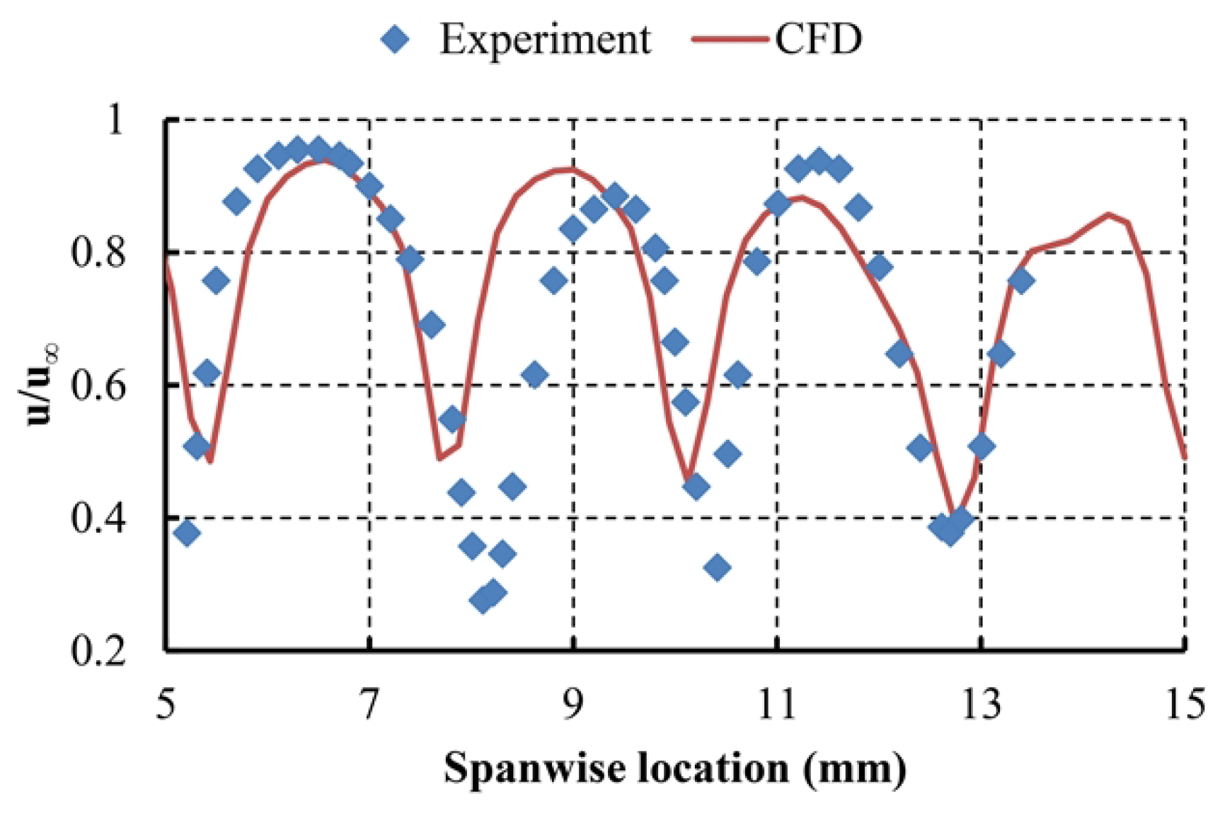
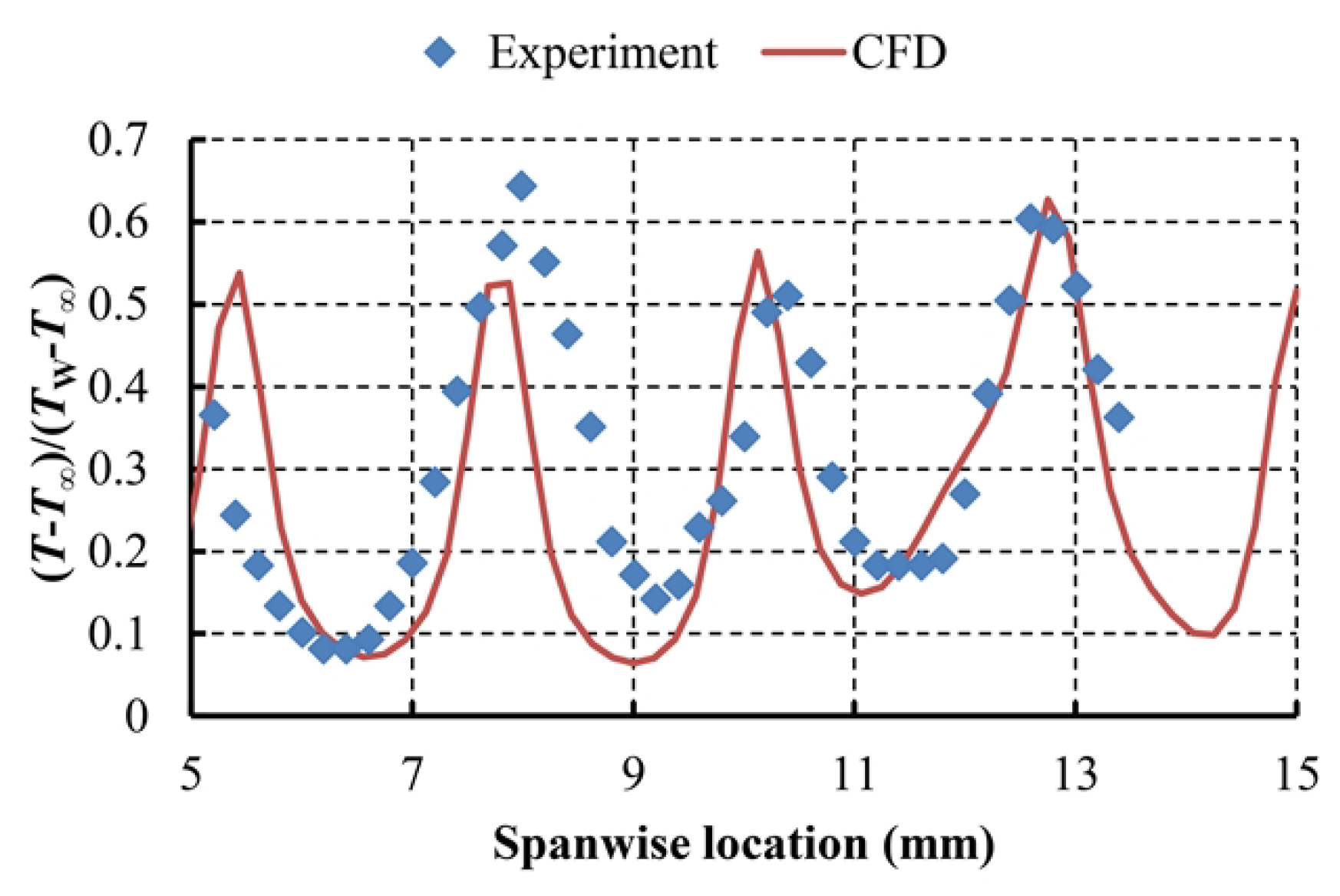
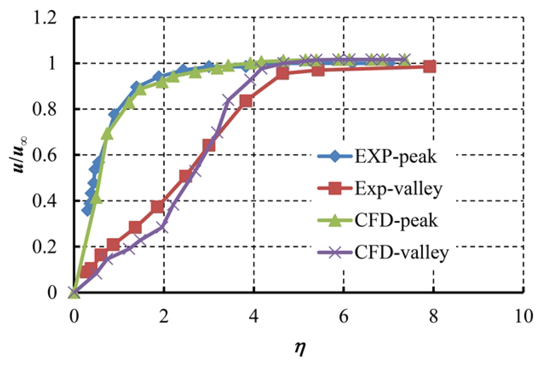
2.2.3. Comparison of Computational and Experimental Results

In the wind tunnel test, X velocity was $u_{\infty }=0.34$ m/s. Temperature difference between airflow and heated plate was $T_W-T_{\infty }=30$ K. Spanwise distribution of dimensionless X velocity and temperature with $x=295$ mm and $z=5$ mm was measured in experiment. Experimental and CFD result comparisons are shown in Figure 5 and Figure 6. Dimensionless X velocity is defined as follows:

$$\overline{u}=u/u_{\infty }$$

(10)

where $u$ is the X velocity of fluid, and $u_{\infty }$ is the free stream velocity. Dimensionless temperature is defined as follows:

$$\overline{T}=\left(T-T_{\infty }\right)/\left(T_W-T_{\infty }\right)$$

(11)

where $T$ is the fluid temperature, $T_{\infty }$ is the free stream temperature, and $T_{\infty }$ is the wall temperature.

From the comparisons, it can be seen that the CFD results are in good agreement with the experimental results. CFD can accurately calculate the peak value and corresponding spanwise position of velocity distribution and temperature distribution.

From Figure 5, it can be found that there are several velocity peaks and valleys. Figure 7 and Figure 8 show the comparisons of velocity and temperature distribution in the boundary layer of CFD and experimental results. The X-axis $\eta$ represents the dimensionless height above plate, which is defined as:

$$\eta =z{\left(u_{\infty }/\nu x\right)}^{1/2}$$

(12)

where $\nu$ is the kinematic viscosity.

Figure 7 and Figure 8 show that CFD can accurately calculate the velocity and temperature distributions in the boundary layer. Therefore, using this CFD method for subsequent research is appropriate.

3. Results and Discussion

In order to investigate the effects of airflow velocity, airflow temperature, and temperature difference, a set of cases was studied using the CFD method.

Table 1. Computation conditions for different cases.

Case No.	Airflow Velocity ${\mathit{u}}_{\mathit{\infty }}$ (m/s)	Airflow Temperature ${\mathit{T}}_{\mathit{\infty }}$ (K)	Temperature Difference ${\mathit{T}}_{\mathit{W}}-{\mathit{T}}_{\mathit{\infty }}$ (K)	Reynolds Number
Case 1	0.63	238	30	5.44 × 104
Case 2		288		3.95 × 104
Case 3		338		3.02 × 104
Case 4		238	60	4.91 × 104
Case 5		288		3.62 × 104
Case 6		338		2.81 × 104
Case 7	0.34	238	30	2.94 × 104
Case 8		288		2.13 × 104
Case 9		338		1.63 × 104
Case 10		238	60	2.65 × 104
Case 11		288		1.96 × 104
Case 12		338		1.52 × 104

provides the computation conditions for different cases. The Reynolds number is based on the unit length.

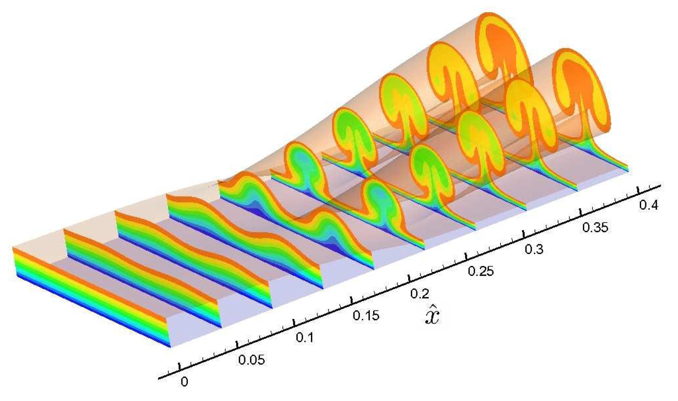
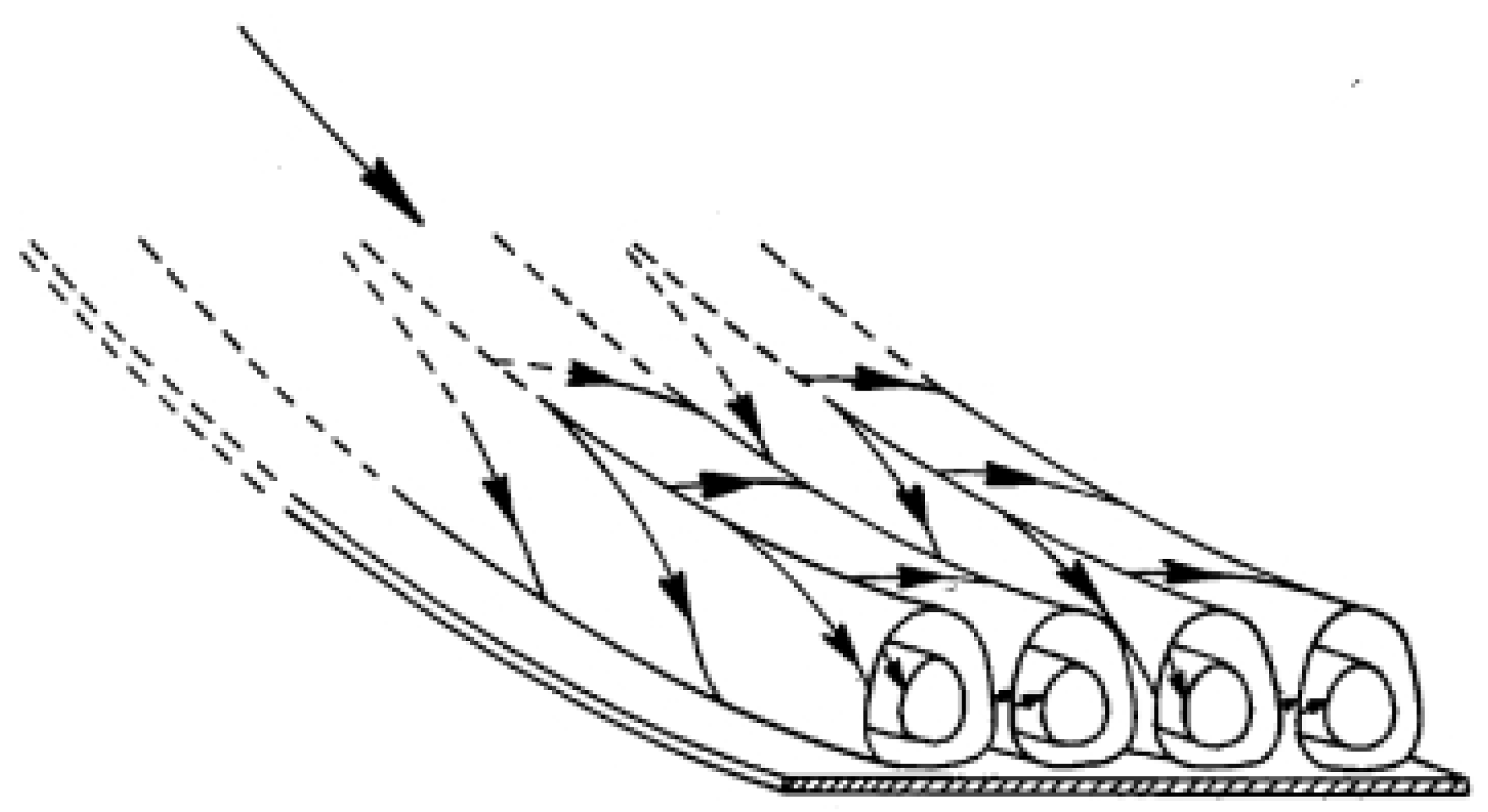
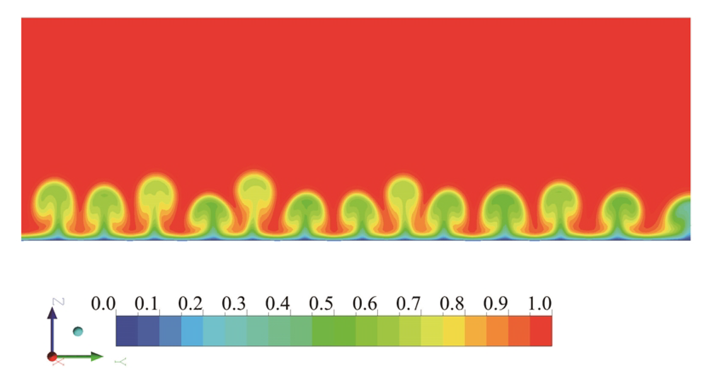
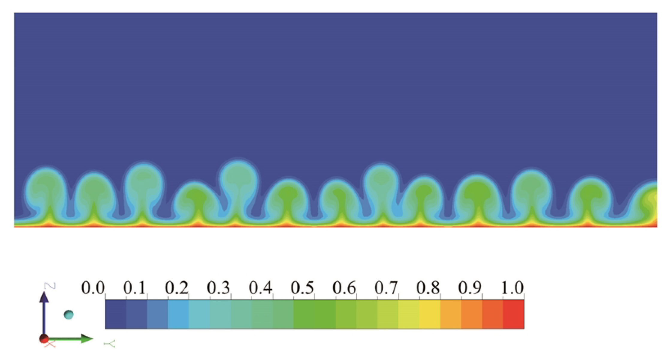
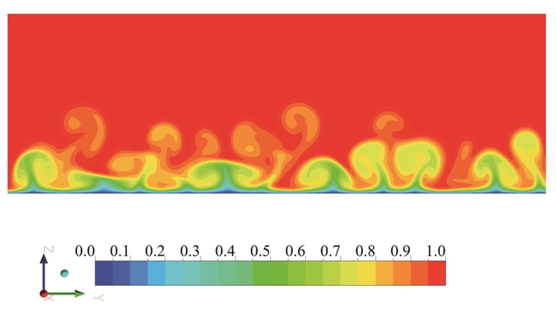
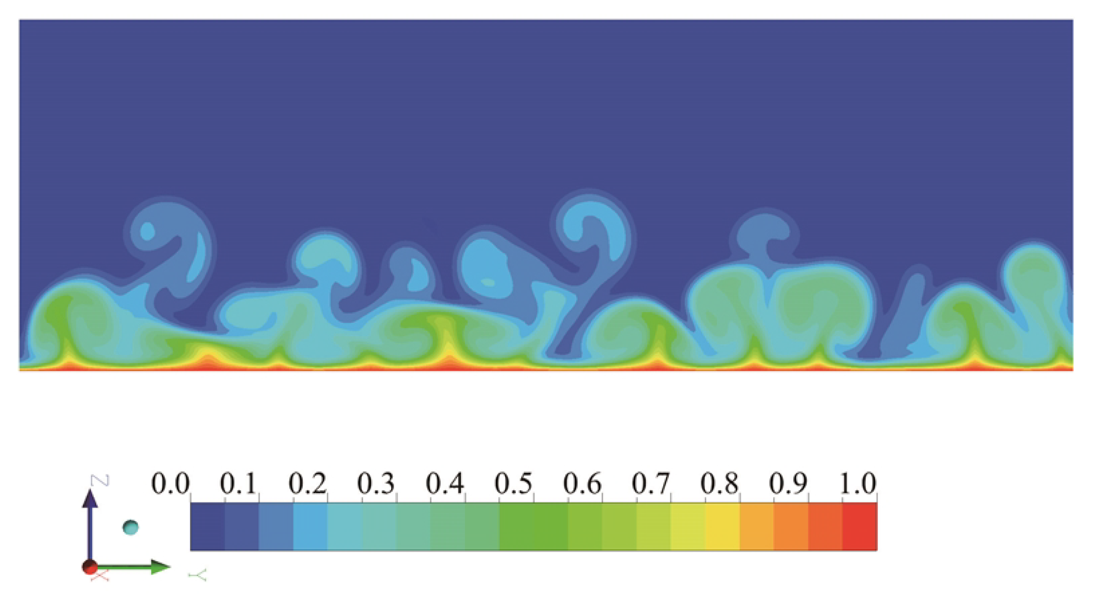
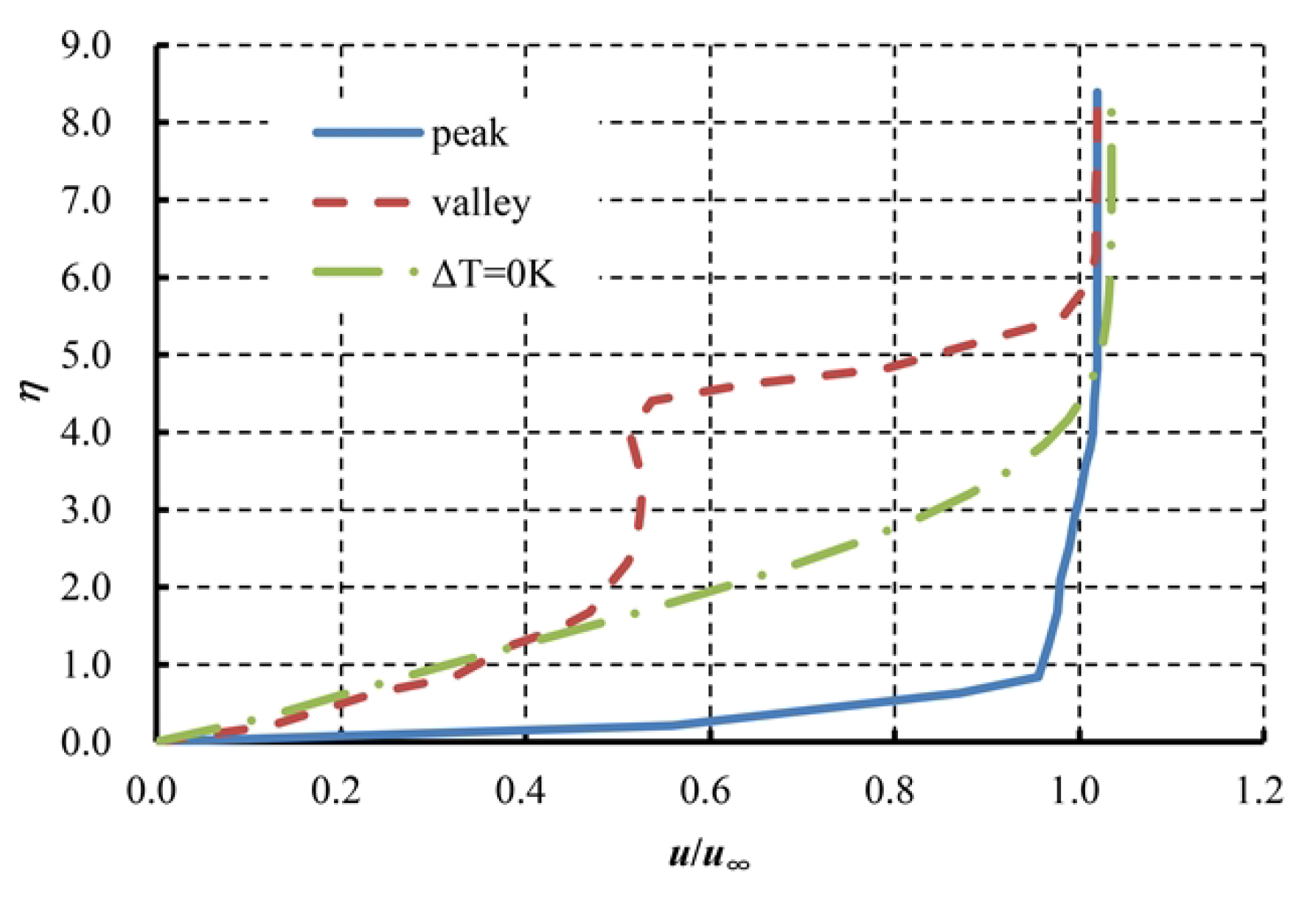
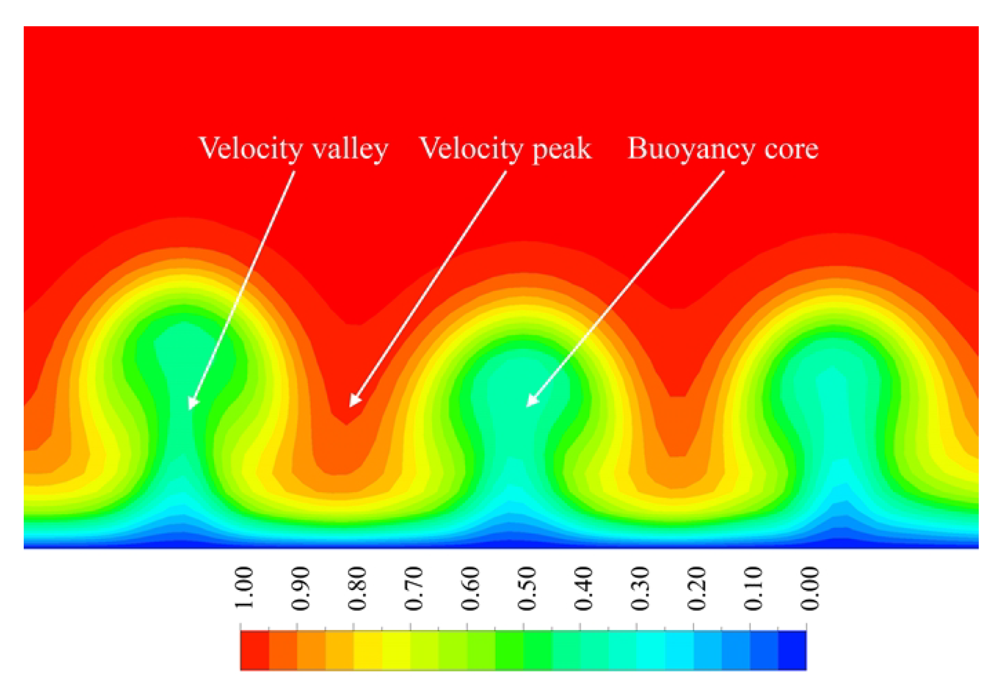
3.1. Flow Visualization

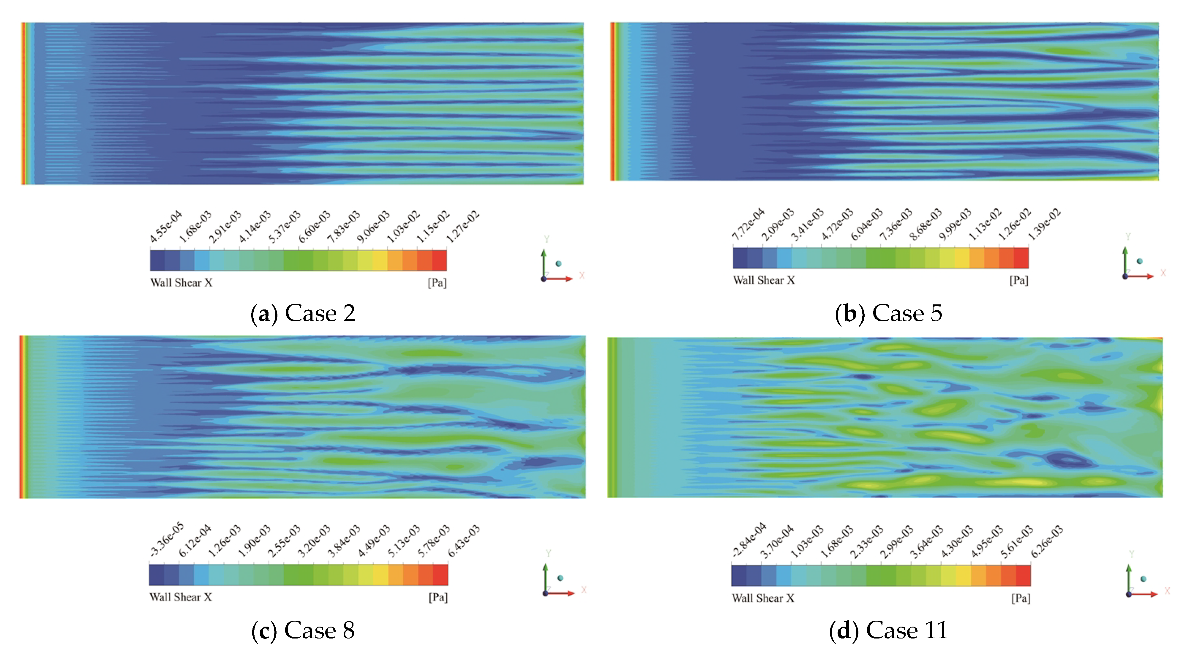
First, we take case 5 as an example to analyze the flow structure. Other cases in this study also have similar flow structures. Figure 9 shows the contour of the X-direction wall shear on the heated plate. There were several wall shear stripes along the flow direction. If the flat plate is not heated, the contour should be uniform. This indicates that the flow is no longer two-dimensional. There should be a three-dimensional flow structure above the heated plate.

As shown in Figure 9, the flow above the heated plate can be divided into three regions. At small downstream distances from the leading edge of the plate, the buoyancy effect was not obvious due to the gas just starting to heat up. This was a laminar forced convection region in which the Görtler vortex had not yet formed, and the flow remained two-dimensional.

As the flow continued to develop downstream, vortices began to appear when a critical distance was reached. Mushroom-like flow structures began to appear across the heated plate, forming a three-dimensional flow. As the flow further developed, the Görtler vortices gradually became stable, forming stable vortices pairs whose axes were in the streamwise direction, one rolling clockwise and another counterclockwise with a plume-like flow in the center. Figure 10 and Figure 11 show the dimensionless X-direction velocity $\overline{u}$ and temperature $\overline{T}$ contours in the y–z plane at a distance of 0.6 m from the leading edge of the flat plate.

After the stable region, vortices began to twist and merge until they broke down, forming an unstable vortex region of several cells created from the growth of the individual vortices. Downstream of this region, the cells started mixing with each other in a random fashion, and the flow developed slowly into a two-dimensional, fully developed turbulent flow. Figure 12 and Figure 13 show the dimensionless X-direction velocity $\overline{u}$ and temperature $\overline{T}$ contours in the y–z plane at a distance of 0.9 m from the leading edge of the flat plate.

Figure 14 shows the X-direction wall shear contour on the plate under other conditions. As shown in the figures, they had similar flow structures, as shown in Figure 9. It also could be found that, with the increased temperature difference or decreased flow velocity, Görtler vortices intensities increased and broke down earlier.

3.2. Wall Shear

The existence of the Görtler vortex led to a change in the velocity distribution in the boundary layer and affected the magnitude of the wall shear stress. Figure 15 shows the comparison of wall shear stress under different conditions with an inflow velocity of 0.63 m/s. As shown in the figure, the distribution of shear stress at the valley position was closer to that of an unheated plate. However, at the peak position, the shear stress rapidly increased. The growth rate is much higher than that of an unheated plate.

The reason for this phenomenon is that the counter-rotating Görtler vortex pair induces a negative z-direction velocity at the peak position, which increases the momentum exchange inside and outside the boundary layer, making the velocity distribution closer to the turbulent boundary layer. At the valley position, under the influence of buoyancy, a positive z-direction velocity is generated, which inhibits momentum exchange, and the velocity distribution is closer to the laminar boundary layer.

Figure 15 also shows stark differences in the wall shear in the peaks between the 30 K and 60 K temperature difference cases. Due to the length of the flat plate being only about 1 m, when the temperature difference was 30 K, by the end of the plate, the Görtler vortex was still in a stable development stage and did not break down. The flow was in a transitional stage from laminar to turbulent flow. When the temperature difference was 60 K, the Görtler vortex had already broken above the flat plate. The flow transitioned to complete turbulence. This phenomenon can be seen by comparing Figure 14a,b. When the flow develops into full turbulence, the friction coefficient decreases with the increased Reynolds number. Therefore, the wall shear stress curve corresponding to the temperature difference of 60 K in Figure 15 shows a trend of first increasing and then decreasing. For the 30 K temperature difference curve, the shear stress is always increasing because the flow is in the transition process. If the length of the plate further increases, it can be reasonably expected that the curve will also show a trend of first increasing and then decreasing.

The velocity distribution comparison in the boundary layer with $u_{\infty }=0.63$ m/s is shown in Figure 16. As seen from the figure, at the valley position and close to the wall, the velocity distribution was closer to the laminar flow velocity pattern above the adiabatic wall. Therefore, the wall shear stress was relatively small. At the peak, the velocity gradient near the wall was much greater than that of the laminar boundary layer, resulting in a rapid increase in shear stress.

We also found that while the boundary closely resembled a laminar boundary layer in the valley up to a certain point, there was a sharp departure afterward. The reason for this phenomenon can be seen in Figure 17. Görtler vortices have a periodic mushroom-like flow structure. Between the two “mushrooms” is the velocity peak. In the central part of the mushroom flow structure, the flow is driven by buoyancy mostly and is the buoyancy core of the Görtler vortex. At this position, the flow has a large z-direction velocity, and the height of the boundary layer increases rapidly, resulting in an insignificant increase in X-direction velocity with height. This results in the velocity distribution shown in Figure 16.

The Görtler vortex led to an earlier transition of the plate flow in some areas, and the wall shear stress was greater, which increased the viscous friction drag coefficient of the plate. For the case where the incoming velocity was 0.63 m/s, the viscous drag coefficient $C_{Df}=0.00468$ when the temperature difference is 0 K. When the temperature difference is 30 K, the viscous drag coefficient $C_{Df}=0.01017$. When the temperature difference increased to 60 K, the viscous drag coefficient also increased to $C_{Df}=0.01214$, almost three times that of the 0 K temperature difference state.

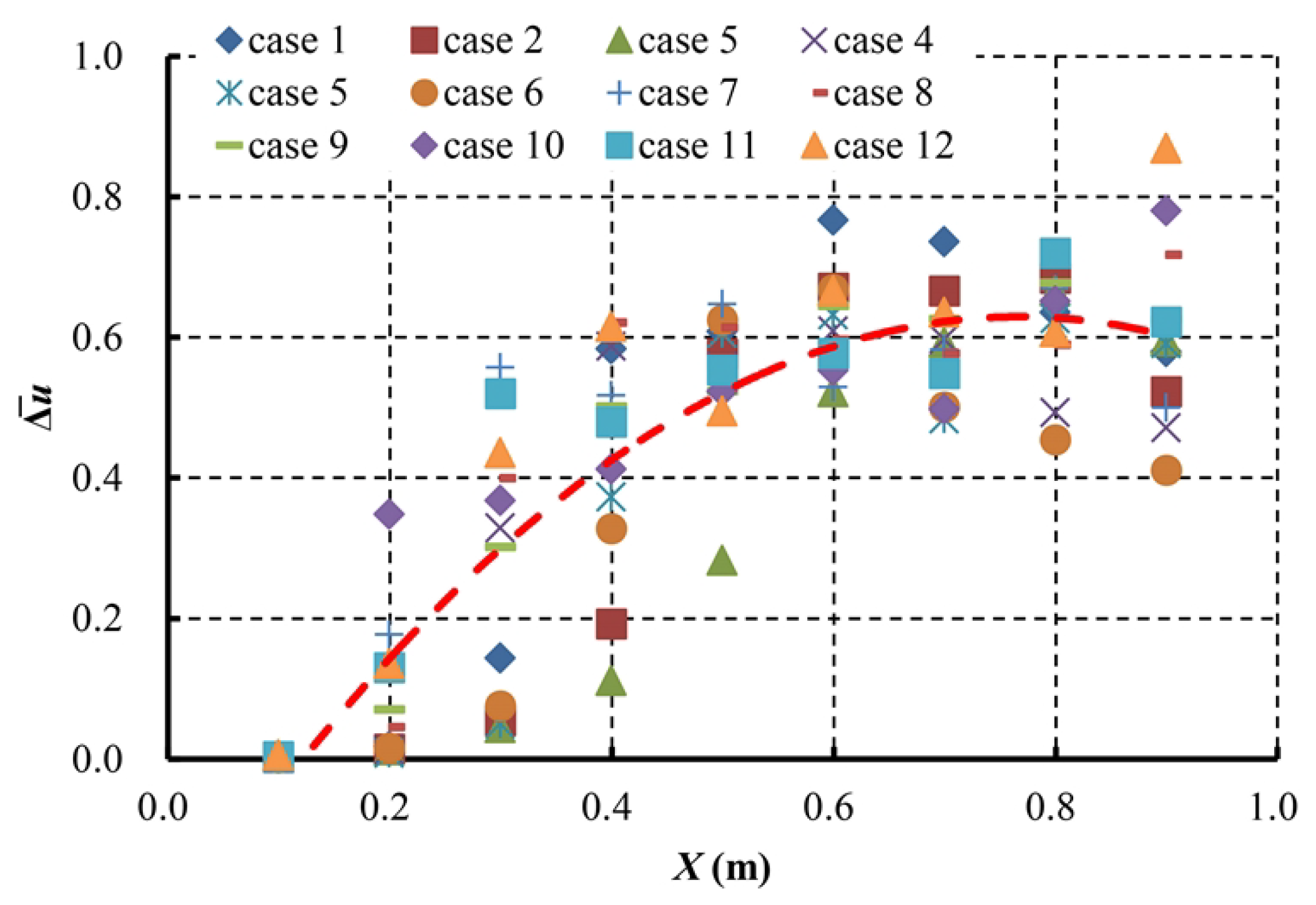
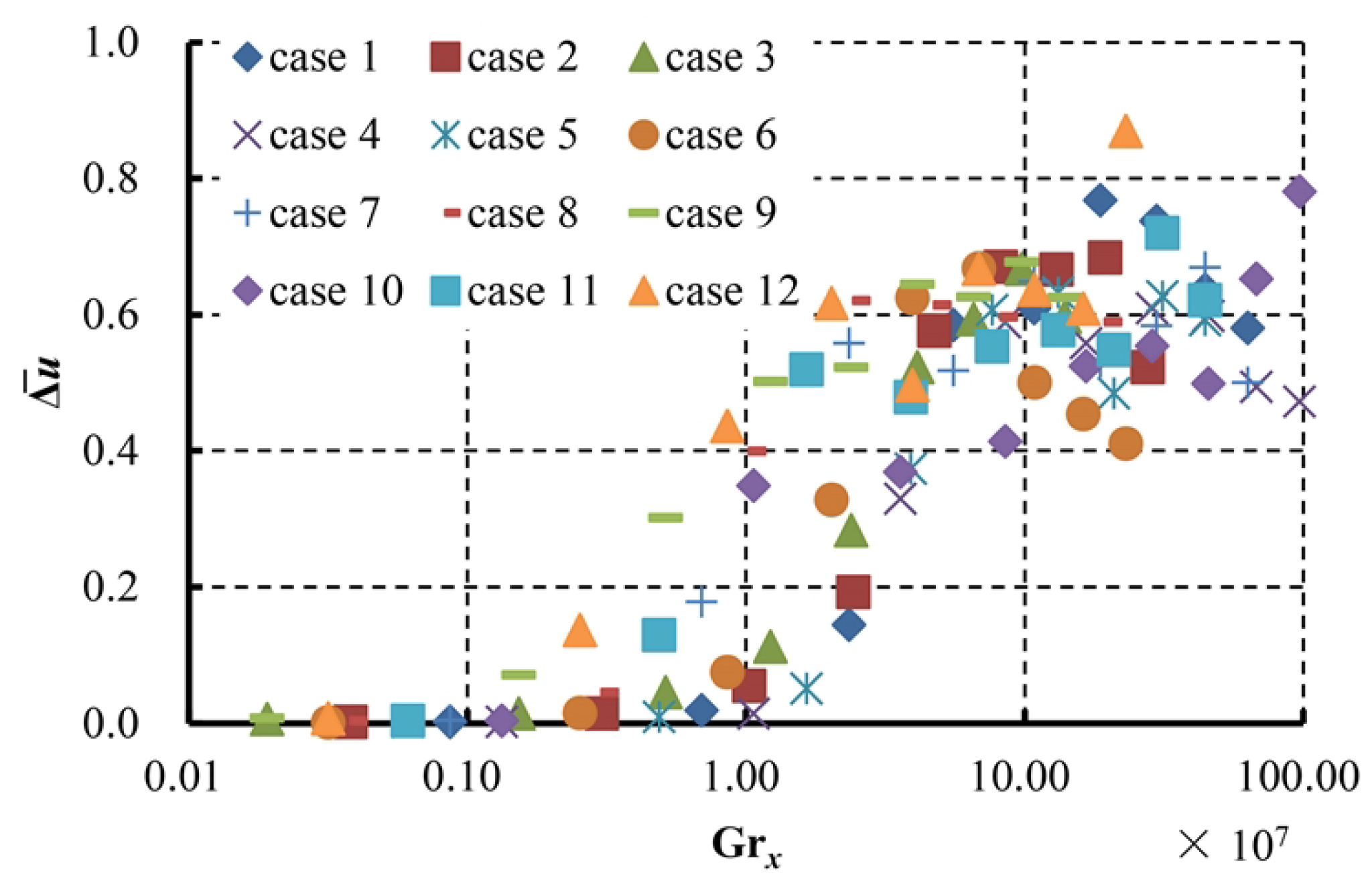
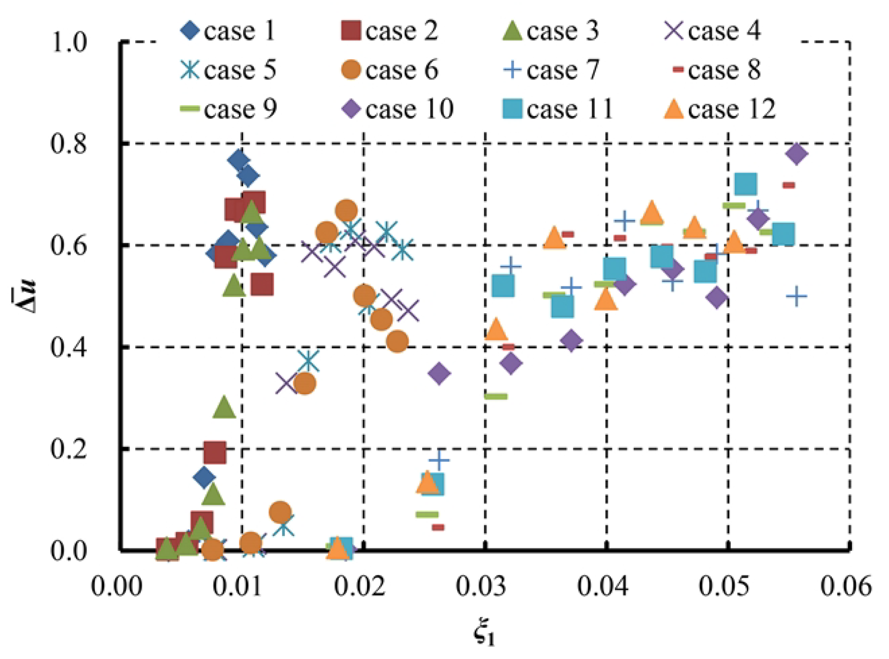
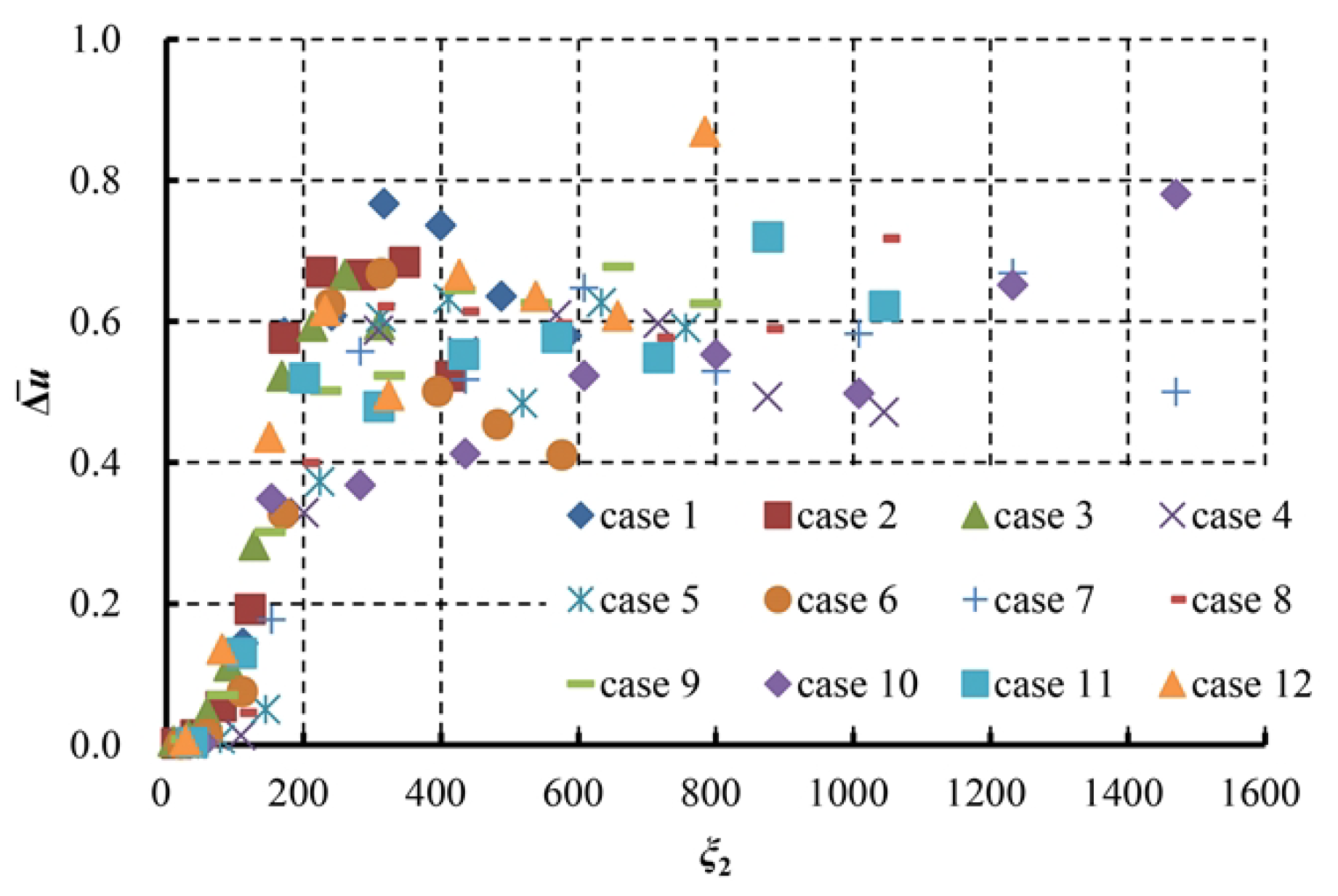
3.3. Buoyancy Parameter

For an adiabatic flat plate, the flow state mainly depends on the local Reynolds number, which is defined as follows:

$${\mathrm{Re}}_x=u_{\infty }x/\nu$$

(13)

For buoyancy-driven flow, the flow state mainly depends on the local Grashof number, which is defined as follows:

$${\mathrm{Gr}}_x=g\beta \left(T_W-T_{\infty }\right)x^3/{\nu }^2$$

(14)

where, $g$ is gravitational acceleration, and $\beta$ is a volumetric coefficient of thermal expansion.

However, there is a lack of reasonable buoyancy parameters for the generation and fragmentation of buoyancy-driven Görtler vortices. In order to propose a reasonable buoyancy parameter, it is first necessary to define a parameter that represents the strength of Görtler vortices. According to the results in Section 3.1, the presence of Görtler vortices can cause fluctuations in the x-velocity along the spanwise direction. Therefore, the fluctuation value of x-velocity can be used as a reasonable parameter to evaluate the strength of Görtler vortices, which is defined as follows:

$$\overline{\Delta u}=\frac{u_{\max }-u_{\min }}{u_{\infty }}$$

(15)

where $u_{\max }$ is the maximum value of the x-velocity spanwise at some X location 5 mm above the plate. $u_{\min }$ is the minimum value of the x-velocity spanwise at some X location 5 mm above the plate. As shown in Figure 18, the value of $\overline{\Delta u}$ is very small near the leading edge of the plate, indicating that the Görtler vortex has not formed and the flow is two-dimensional. As X increases, $\overline{\Delta u}$ rapidly increases. This indicates that the buoyancy-induced generation of Görtler vortices transforms two-dimensional flow into three-dimensional flow. With the increase in X, $\overline{\Delta u}$ gradually increased, and the strength of the Görtler vortex steadily increased. When X reached a critical value, $\overline{\Delta u}$ began to decrease. This is because the Görtler vortices begin to break down, and the flow gradually transforms into a completely turbulent flow, regaining two-dimensional characteristics.

Figure 19 and Figure 20 show the relationship of $\overline{\Delta u}$ with ${\mathrm{Re}}_x$ and ${\mathrm{Gr}}_x$. We found no obvious pattern between $\overline{\Delta u}$ and ${\mathrm{Re}}_x$, ${\mathrm{Gr}}_x$. This indicates that parameters ${\mathrm{Re}}_x$ and ${\mathrm{Gr}}_x$ cannot independently determine the flow state of the Görtler vortex.

As can be seen from the figure, under different calculation conditions, the X position at which the $\overline{\Delta u}$ value reaches its maximum value is different. Since the buoyancy-driven Görtler vortex is related to both the Reynolds and Grashof numbers, it can be reasonably predicted that the buoyancy parameters should be a combination of the two. Two combined buoyancy parameters are investigated in the present research. They are defined as follows:

$${\xi }_1={\mathrm{Gr}}_x/{\mathrm{Re}}_x^{2.5}$$

(16)

$${\xi }_2={\mathrm{Gr}}_x/{\mathrm{Re}}_x^{1.5}$$

(17)

Figure 21 shows the calculation results of $\overline{\Delta u}$ and ${\xi }_1$ under different conditions. As shown in the figure, $\overline{\Delta u}$ first increased and then decreased as ${\xi }_1$ increased, but the range of ${\xi }_1$ values corresponding to the maximum value of $\overline{\Delta u}$ varied greatly. This indicates that ${\xi }_1$ has little reference significance for predicting the development status of Görtler vortices and is not a suitable buoyancy parameter.

Figure 22 shows the calculation results of $\overline{\Delta u}$ and ${\xi }_2$ under different conditions. From the figure, it can be seen that before $\overline{\Delta u}$ reached its maximum value, the variation pattern of $\overline{\Delta u}$ with ${\xi }_2$ remained basically consistent under different calculation conditions. When $\overline{\Delta u}$ reached its maximum value, the corresponding ${\xi }_2$ was also basically the same. This indicates that ${\xi }_2$, as a buoyancy parameter, has high rationality for describing buoyancy-driven Görtler vortex flow.

Figure 23 shows the calculation results of $\overline{\Delta u}$ and ${\xi }_2$ before taking the maximum value of ${\xi }_2$ in logarithmic coordinates. As shown in the figure, when the ${\xi }_2$ value is 200, $\overline{\Delta u}$ reaches its maximum value. Therefore, ${\xi }_2=200$ can serve as a criterion for the complete development of buoyancy-driven Görtler vortices. If $\overline{\Delta u}=0.1$ is used as the criterion for the start of the Görtler vortex, then ${\xi }_2=100$ can be a good basis.

4. Conclusions

This study conducted 12 cases of CFD calculations with three different inflow temperatures, two inflow velocities, and two temperature differences on a flat plate flow. The results showed that when the temperature of the flat plate was higher than the inlet temperature, buoyancy would generate Görtler vortices above the flat plate. The most significant feature of buoyancy-driven Görtler vortices is the stable vortex pairs, whose axes are in the streamwise direction, one rolling clockwise and another counterclockwise with a plume-like flow in the center.

The counter-rotating Görtler vortex pair induces a negative z-direction velocity at the peak position, which increases the momentum exchange inside and outside the boundary layer, making the transition occur earlier and changing the velocity distribution in the boundary layer. At the peak position, the velocity distribution is closer to the turbulent boundary layer. The increase in velocity gradient near the wall leads to an increase in the drag coefficient. When the temperature difference is 60 K, the drag coefficient is almost three times that when the temperature difference is 0 K.

The flow state of the heated plate is related to both the Reynolds number and Grashof number. Therefore, the simple Reynolds number and Grashof number can not be used as the basis for judging the flow state alone. By analyzing the calculation results, the combination parameter ${\xi }_2={\mathrm{Gr}}_x/{\mathrm{Re}}_x^{1.5}$ can better determine whether the buoyancy-driven Görtler vortex is fully developed. According to existing calculation results, ${\xi }_2=100$ indicates the beginning of buoyancy-driven Görtler vortices, while ${\xi }_2=200$ indicates the complete development of buoyancy-driven Görtler vortices.

Although the Reynolds number studied in this paper is different from that of the solar UAV, it can be reasonably assumed that the temperature difference between the solar cell and the atmosphere will also change the flow characteristics of the UAV wing, change the position of laminar transition, and lead to increased drag. Therefore, studying the buoyancy-driven Görtler vortex has a high reference value for the aerodynamic design of solar UAVs.

This study focuses on flat plate flow and does not consider the influence of the pressure gradient. In the future, further consideration needs to be given to the impact of the pressure gradient on the stability of buoyancy-driven Görtler vortices in order to make the relevant conclusions more in line with the actual situation.

References

1. Ma, D.L.; Zhang, L.; Yang, M.Q.; Xia, X.; Wang, S. Review of Key Technologies of Ultra-Long-Endurance Solar Powered Unmanned Aerial Vehicle. Acta Aeronaut. Astronaut. Sin. 2020, 41, 623418. (In Chinese) [Google Scholar] [CrossRef]
2. Lun, Y.; Yao, P.; Wang, Y. Trajectory Optimization of SUAV for Marine Vessels Communication Relay Mission. IEEE Syst. J. 2020, 14, 5014–5024. [Google Scholar] [CrossRef]
3. Noll, T.E.; Ishmael, S.D.; Henwood, B.; Perez-Davis, M.E.; Tiffany, G.C.; Madura, J.; Gaier, M.; Brown, J.M.; Wierzbanowski, T. Technical Findings, Lessons Learned, and Recommendations Resulting from the Helios Prototype Vehicle Mishap. In Proceedings of the NATO/RTO AVT-145 Workshop on Design Concepts, Processes and Criteria for UAV Structural Integrity, Florence, Italy, 1 January 2007. [Google Scholar]
4. Rapinett, A. Zephyr: A High Altitude Long Endurance Unmanned Air Vehicle. Master’s Thesis, University of Surrey, Guildford Surrey, UK, 2009. [Google Scholar]
5. Qian, Y. Aerodynamics, 1st ed.; Beihang University Press: Beijing, China, 2004; pp. 15–25. (In Chinese) [Google Scholar]
6. Vinnichenko, N.A.; Uvarov, A.V.; Znamenskaya, I.A.; Ay, H.; Wang, T.-H. Solar car aerodynamic design for optimal cooling and high efficiency. Sol. Energy 2014, 103, 183–190. [Google Scholar] [CrossRef]
7. Zhang, J. Preliminary Study and Experiments on Energy Management of Solar Powered Aircraft. Master’s Thesis, Tsinghua University, Beijing, China, 2005. (In Chinese). [Google Scholar]
8. Natarajan, S.K.; Mallick, T.K.; Katz, M.; Weingaertner, S. Numerical investigations of solar cell temperature for photovoltaic concentrator system with and without passive cooling arrangements. Int. J. Therm. Sci. 2011, 50, 2514–2521. [Google Scholar] [CrossRef]
9. Görtler, H. On the Three-Dimensional Instability of Laminar Boundary Layers on Concave Walls; National Advisory Commitee for Aeronautics: Edwards, CA, USA, 1954.
10. Floryan, J.M.; Saric, W.S. Stability of Gortler Vortices in Boundary Layers. AIAA J. 1982, 20, 316–324. [Google Scholar] [CrossRef]
11. Mitsudharmadi, H.; Winoto, S.H.; Shah, D.A. Development of most amplified wavelength Görtler vortices. Phys. Fluids 2006, 18, 14101. [Google Scholar] [CrossRef]
12. Mitsudharmadi, H.; Winoto, S.H.; Shah, D.A. Secondary instability in forced wavelength Görtler vortices. Phys. Fluids 2005, 17, 74101–74104. [Google Scholar] [CrossRef]
13. Mitsudharmadi, H.; Winoto, S.H.; Shah, D.A. Splitting and merging of Görtler vortices. Phys. Fluids 2005, 17, 124101–124102. [Google Scholar] [CrossRef]
14. Winoto, S.H.; Mitsudharmadi, H.; Shah, D.A. Visualizing Görtler vortices. J. Vis. 2005, 8, 315–322. [Google Scholar] [CrossRef]
15. Tandiono; Winoto, S.H.; Shah, D.A. On the linear and nonlinear development of Görtler vortices. Phys. Fluids 2008, 20, 94101–94103. [Google Scholar] [CrossRef]
16. Tandiono; Winoto, S.H.; Shah, D.A. Wall shear stress in Görtler vortex boundary layer flow. Phys. Fluids 2009, 21, 84101–84106. [Google Scholar] [CrossRef]
17. Tandiono, T.; Winoto, S.H.; Shah, D.A. Spanwise Velocity Component in Nonlinear Region of Görtler Vortices. Phys. Fluids 2013, 25, 104101–104104. [Google Scholar] [CrossRef]
18. Rogenski, J.K.; de Souza, L.F.; Floryan, J.M. Influence of Pressure Gradients on the Evolution of the Görtler Instability. AIAA J. 2016, 54, 2916–2921. [Google Scholar] [CrossRef]
19. Kahawita, R.; Meroney, R. The Influence of Heating on the Stability of Laminar Boundary Layers Along Concave Curved Walls. J. Appl. Mech. 1977, 44, 11–17. [Google Scholar] [CrossRef]
20. Imura, H.; Gilpin, R.R.; Cheng, K.C. An Experimental Investigation of Heat Transfer and Buoyancy Induced Transition from Laminar Forced Convection to Turbulent Free Convection over a Horizontal Isothermally Heated Plate. J. Heat Transf. 1978, 100, 429–434. [Google Scholar] [CrossRef]
21. Moutsoglou, A.; Chen, T.S.; Cheng, K.C. Vortex Instability of Mixed Convection Flow over a Horizontal Flat Plate. J. Heat Transf. 1981, 103, 257–261. [Google Scholar] [CrossRef]
22. Momayez, L.; Dupont, P.; Peerhossaini, H. Effects of vortex organization on heat transfer enhancement by Görtler instability. Int. J. Therm. Sci. 2004, 43, 753–760. [Google Scholar] [CrossRef]
23. Wu, X.; Moin, P. Transitional and turbulent boundary layer with heat transfer. Phys. Fluids 2010, 22, 85101–85105. [Google Scholar] [CrossRef]
24. Menter, F.R.; Kuntz, M.; Langtry, R. Ten Years of Industrial Experience with the SST Turbulence Model. In Proceedings of the 4th International Symposium on Turbulence, Heat and Mass Transfer, Antalya, Turkey, 12–17 October 2003. [Google Scholar]
25. Moharreri, S.S.; Armaly, B.F.; Chen, T.S. Measurements in the Transition Vortex Flow Regime of Mixed Convection Above a Horizontal Heated Plate. J. Heat Transf. 1988, 110, 358–365. [Google Scholar] [CrossRef]
Figure 1. Diagram of buoyancy-driven Görtler vortices.
Aerospace 10 00685 g001
Figure 2. Diagram of Görtler vortices over a concave surface.
Aerospace 10 00685 g002
Figure 3. The heated aluminum plate and axis.
Aerospace 10 00685 g003
Figure 4. Mesh around heated plate.
Aerospace 10 00685 g004
Figure 5. Comparison of velocity distribution.
Aerospace 10 00685 g005
Figure 6. Comparison of temperature distribution.
Aerospace 10 00685 g006
Figure 7. Comparison of velocity distributions in boundary layer.
Aerospace 10 00685 g007
Figure 8. Comparison of temperature distributions in boundary layer.
Aerospace 10 00685 g008
Figure 9. Contour of X-direction wall shear on heated plate.
Aerospace 10 00685 g009
Figure 10. Contour of dimensionless velocity u ¯ with x = 0.6 m.
Aerospace 10 00685 g010
Figure 11. Contour of dimensionless temperature T ¯ with x = 0.6 m.
Aerospace 10 00685 g011
Figure 12. Contour of dimensionless velocity u ¯ with x = 0.9 m.
Aerospace 10 00685 g012
Figure 13. Contour of dimensionless temperature T ¯ with x = 0.6 m.
Aerospace 10 00685 g013
Figure 14. Contour of X-direction wall shear of different cases.
Aerospace 10 00685 g014
Figure 15. Wall shear comparison of different conditions.
Aerospace 10 00685 g015
Figure 16. Comparison of velocity distribution in boundary layer.
Aerospace 10 00685 g016
Figure 17. Mushroom-like Görtler vortex structure.
Aerospace 10 00685 g017
Figure 18. Relationship of x-velocity fluctuation and X position (dashed line represents the trend line of the average value at each position).
Aerospace 10 00685 g018
Figure 19. Relationship of x-velocity fluctuation and Rex.
Aerospace 10 00685 g019
Figure 20. Relationship of x-velocity fluctuation and Grx.
Aerospace 10 00685 g020
Figure 21. Relationship of x-velocity fluctuation and buoyancy parameter ξ 1 .
Aerospace 10 00685 g021
Figure 22. Relationship of x-velocity fluctuation and buoyancy parameter ξ 2 .
Aerospace 10 00685 g022
Figure 23. Calculation results of Δ u ¯ and ξ 2 .
Aerospace 10 00685 g023