Design and Experimental Validation of an Adaptive Multi-Layer Neural Network Observer-Based Fast Terminal Sliding Mode Control for Quadrotor System

Abstract

This study considers the numerical design and practical implementation of a new multi-layer neural network observer-based control design technique for unmanned aerial vehicles systems. Initially, an adaptive multi-layer neural network-based Luenberger observer is designed for state estimation by employing a modified back-propagation algorithm. The proposed observer’s adaptive nature aids in mitigating the impact of noise, disturbance, and parameter variations, which are usually not considered by conventional observers. Based on the observed states, a nonlinear dynamic inversion-based fast terminal sliding mode controller is designed to attain the desired attitude and position tracking control. This is done by employing a two-loop control structure. Numerical simulations are conducted to demonstrate the effectiveness of the proposed scheme in the presence of disturbance, parameter uncertainty, and noise. The numerical results are compared with current approaches, demonstrating the superiority of the proposed method. In order to assess the practical effectiveness of the proposed method, hardware-in-loop simulations are conducted by utilizing a Pixhawk 6X flight controller that interfaces with the mission planner software. Finally, experiments are conducted on a real F450 quadrotor in a secured laboratory environment, demonstrating stability and good tracking performance of the proposed MLNN observer-based SMC control scheme.

1. Introduction

Recently, unmanned aerial vehicles (UAVs) gained considerable attention among engineers and researchers, with applications in several industries such as environmental monitoring, disaster response, precision agriculture, infrastructure inspection, and numerous other domestic applications [1,2]. Recent technological advancements in UAVs have enabled cost-effective autonomous navigation [3]. Controlling UAVs poses a greater challenge due to the presence of adverse forces like aerodynamic factors (such as wind gusts) and sensor noise, which can potentially cause instability or vehicle crash. Hence, addressing these issues is crucial for ensuring safe navigation.

In the existing work, a variety of control algorithms and architecture have been presented to improve the tracking accuracy of UAV systems. The strategies encompass adaptive control [4], reinforcement learning [5], data-driven based fault-tolerant control [6], fuzzy fractional PID controller [7], and adaptive neural network based control [8]. Furthermore, studies have explored ways to enhance control strategies for accurately following quadrotor flight paths under the influence of disturbances. Some recent control techniques include disturbance observer based H∞ control proposed in [9], disturbance observer-based control for intense maneuvering [10], a non-singular finite-time tracking controller using disturbance observers [11], robust backstepping sliding mode control [12], adaptive finite-time backstepping control which estimates disturbance [13], linear quadratic controllers with integral action [14], Fast Terminal Sliding Mode Controller (FTSMC) [15], and adaptive fuzzy control integrated with finite-time control methods [16].

To develop an efficient control system for UAVs, it is crucial to have accurate understanding of the plant states in order to improve control and navigation. While it is possible to use suitable sensors to collect this data, their expensive price and susceptibility to sensor noise and external influences make this method unfeasible in some situations. To solve this problem, various observer- schemes are proposed for UAV systems, such as Kalman filters based state estimation [17,18,19], sliding mode observers [20,21], and high-gain observers [22,23,24]. Nevertheless, they come with certain limitations. The classical Kalman filter requires the complete and accurate dynamics of the system, whereas the Extended Kalman Filter (EKF) and Unscented Kalman Filter (UKF) extends the Kalman filter to handle non-linearity—through linearization or unscented transforms. While classical Kalman filters rely on the accurate system model to provide precise state estimates, they can exhibit high susceptibility to noise and parameter variations. On the other hand, sliding mode observers (SMOs) and high-gain observers (HGOs) are robust to model uncertainties and require a general model structure. However, SMO can suffer from chattering, which introduces high-frequency oscillations, while HGOs are sensitive to noise and require precise gain tuning to prevent instability or degraded performance.

Neural network (NN)-based methods have emerged as potential solutions to overcome the constraints of traditional observers. These methods have become more important in UAV applications [25,26], which demand extremely reliable control and state estimation strategies. In recent years, several NN-observer-based methods have been proposed. For example, the authors in [27] designed fuzzy model predictive control utilizing an NN observer for a constrained hypersonic vehicle. The work in [28] presented a disturbance observer employing a Radial Basic Neural Network (RBFNN) for estimating unknown disturbances for tracking control of multiple UAVs, ensuring finite-time convergence and distributed coordination. Similarly, [29], introduces a disturbance observer based on RBFNN for controlling the attitude and altitude of a UAV amidst disturbances and model uncertainties. In [30], an SMO-based NN method is introduced for a quadcopter to mitigate the impacts of bounded disturbances. In [31], an intelligent sensor scheme based on NN is proposed for attitude estimation within a Global Positioning System (GPS) navigation model, which enhances navigation accuracy by compensating for delay-dependent errors. In [32], a Single Hidden Layer Neural Network (SHLNN)-based observer is suggested for a quadrotor UAV, incorporating a sigmoid activation function to enhance robustness against measurement noise. To address disturbances and uncertainty, a controller using an NN observer is proposed for a missile proposed in [33] holding worthwhile results. Additionally, [34] introduces a multi-layer neural network-based observer for estimating the states of an induction motor. In [35] a disturbance observer is combined with a multi-layer exponential sliding mode controller to address disturbances and parameter uncertainties encountered in a UAV. In [36], a deep learning-based Kalman filter for state estimation in multi-rotor UAVs is proposed and evaluated under the influence of noise. In [37], a single-layer neural network-based observer for a UAV using a back-propagation weight update law is used to eliminate disturbances effects. The work in [38] introduces a back-propagation-based attitude control of a quadrotor, with the study focusing solely on one varying parameter, namely mass variation, in their simulation results. The study in [39] integrates an adaptive neural network and an extended state observer to handle system uncertainties and external disturbances. The proposed observer scheme employs a SHLNN to estimate the disturbances.

Although many control techniques have been designed and tested, most of these approaches are primarily validated through numerical simulations rather than actual real-world applications. This gap emphasizes the necessity for more actual testing and validation in order to connect theoretical modes and operational performance, ensuring the reliability and effectiveness of quadrotor systems in diverse applications. Some recent work on real-time implementation of control algorithms on UAV based on full state feedback includes the implementation of second-order SMC in [40], integral backstepping-based SMC in [41], super-twisting SMC [42,43], adaptive PID control in [44], and model predictive control in [45]. The study in [46] investigates three nonlinear control methods: an existing strategy, Nonlinear Dynamic Inversion (NDI), and Incremental NDI (INDI) for stabilizing a tail-sitter UAV during hover. These were simulated and validated using Hardware-in-the-Loop (HITL) and experimental flight test results. Despite the mentioned scheme has been successfully deployed. However, there is still room for investigation specifically in the presence of unmeasured system states, measurement noise, and perturbation.

This research introduces an adaptive multi-layer neural network (MLNN) observer-based fast terminal SMC scheme for quadrotor UAVs assuming that only the positions of the plant are measured. Initially, the adaptive MLNN observer is employed for estimating the system’s states accurately. Subsequently, the estimated state information is utilized by the nonlinear dynamic inversion (NDI) based fast terminal SMC law to enhance system robustness against unmodeled dynamics and perturbation. The Lyapunov stability proof of the proposed MLNN observer is also provided, which is an extension of the Lyapunov proof for a single-layer NN proposed in [34]. To show the practical applicability of the suggested technique, hardware-in-loop simulations are performed using Pixhawk 6X flight controller and mission planner software. Finally, tests are performed on real quadrotor F450 system to show the efficacy of the suggested scheme. The key contributions of the proposed method are detailed below:

• In comparison to the state observers cited in [9,17,22], the designed MLNN observer can estimate the system state information without requiring precise knowledge of the system dynamics and ensures finite-time convergence.
• The NDI-based fast terminal SMC method offers significant benefits in terms of robustness, convergence speed, handling nonlinear dynamics, computational efficiency, and reduced chattering.
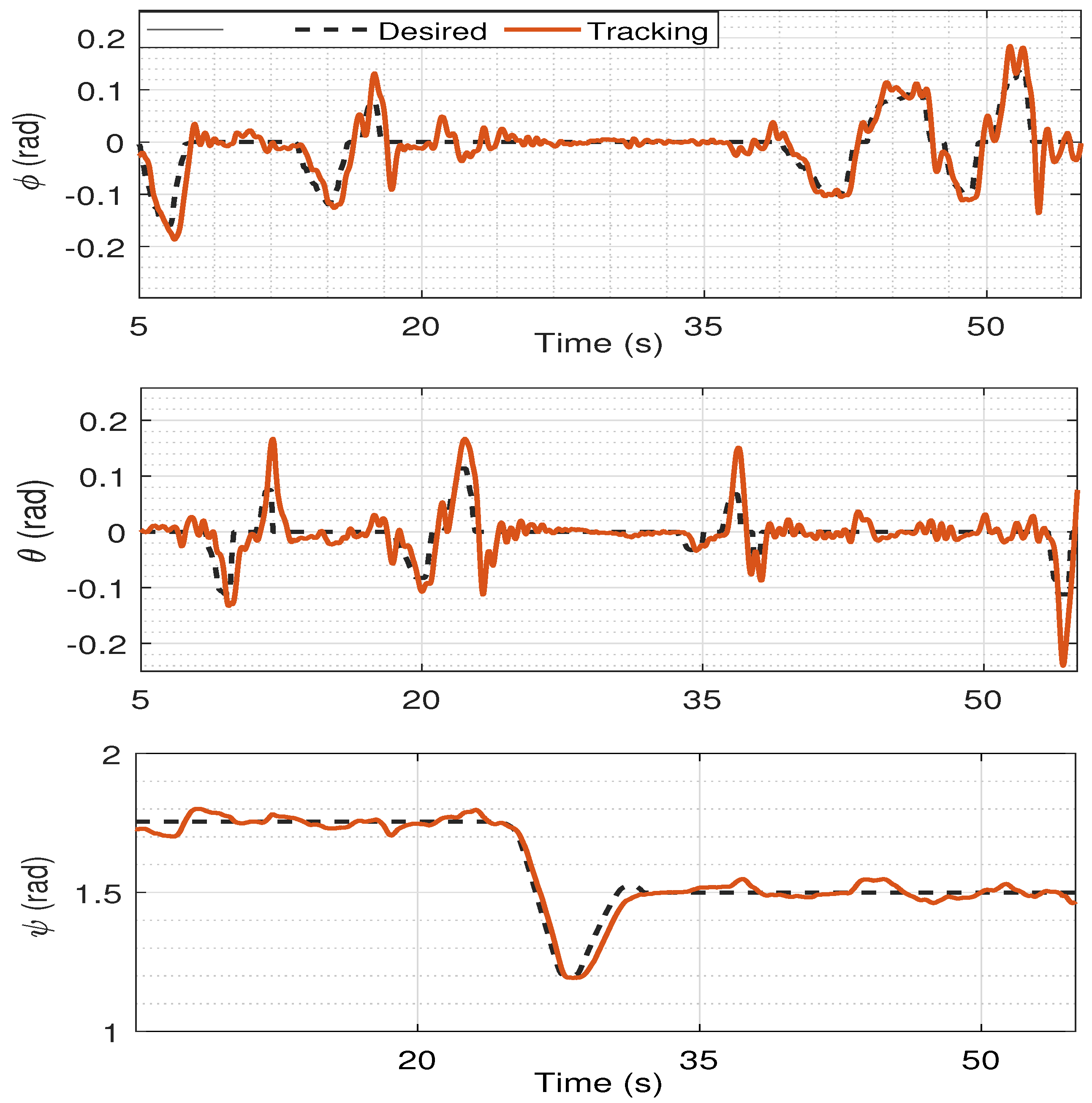
• The hardware-in-loop simulation (HILS) results using Pixhawk 6X flight controller demonstrate good performance of the proposed scheme. In addition, flight tests performed on a real quadrotor demonstrate commendable tracking accuracy.

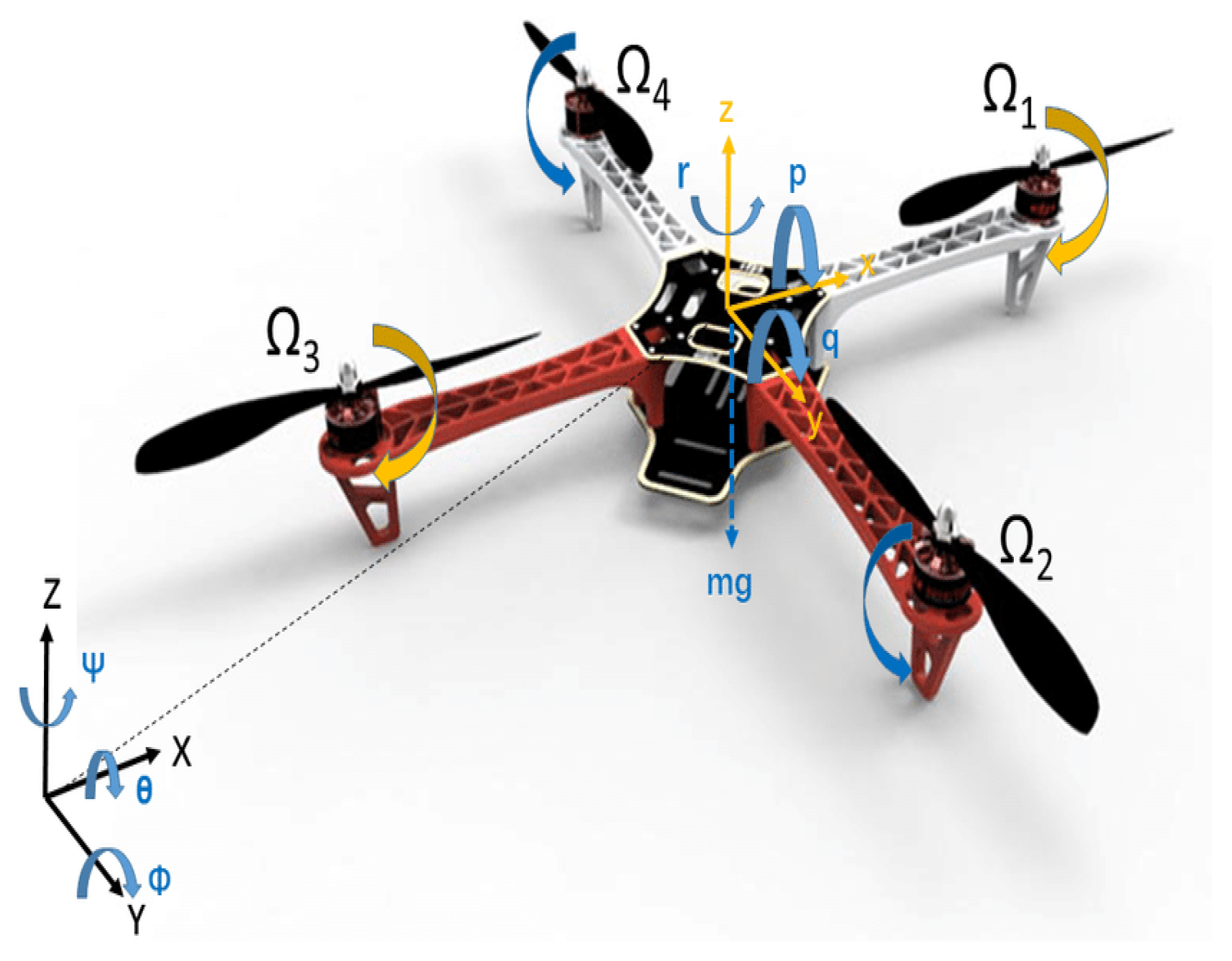
2. Dynamics of Quadrotor UAV

A quadrotor possesses six DOF but is equipped with only four propellers, rendering it an under-actuated system. The assumptions outlined for the quadrotor in this study are taken from [47]. A quadrotor UAV encompasses twelve states, namely, [$x, y, z, \dot{x}, \dot{y}, \dot{z}, \varphi , \theta , \psi , p, q, r]$, where $x, y$, and z represent the translational positions, while $\varphi , \theta$ and $\psi$, denote the roll, ptich and yaw angles, and $p, q$ and r, are their angular velocities Figure 1 shows the structure of an F450 quadrotor.

Its nonlinear equations consists of a rigid body kinematic, dynamic, control effectiveness and propulsor model as follows.

2.1. Kinematic Model

Lets $p_e={\left[\begin{array}{ccc}x& y& z\end{array}\right]}^T$ be the position vector and $v_e={\left[\begin{array}{ccc}\dot{x}& \dot{y}& \dot{z}\end{array}\right]}^T$ denotes the velocity vector in an inertial frame:

$${\dot{p}}_e=v_e$$

(1)

Similarly, ${\mathrm{\Theta }}_b={\left[\begin{array}{ccc}\varphi & \theta & \psi \end{array}\right]}^T$ denotes the attitude vector and ${\omega }_b={\left[\begin{array}{ccc}p& q& r\end{array}\right]}^T$ represents the velocity vector in body fixed frame. The relationship between attitude rate and angular velocities is given as

$${\dot{\mathrm{\Theta }}}_b=R_W{\omega }_b$$

(2)

where

$$R_w=\left[\begin{array}{ccc}1& S_{\varphi }{T}_{\theta }& C_{\varphi }{T}_{\theta }\\ 0& C_{\varphi }& -S_{\varphi }\\ 0& {\displaystyle \frac{S_{\varphi }}{C_{\theta }}}& {\displaystyle \frac{C_{\varphi }}{C_{\theta }}}\end{array}\right]$$

(3)

where $\varphi , \theta$ and $\psi$ denote the roll, pitch and yaw angle, and $p, q$ and r represents their angular rates.

2.2. Dynamics Model of Quadrotor System

The position dynamics is represented as:

$${\dot{v}}_e=m{G}_e+R_e(T_e+F_{de})$$

(4)

where $G_e={[0,0,-g]}^T, T_e={[0,0,T_1]}^T$, $T_1$ represents the total thrust developed by the propellers and is unidirectional, $F_{de}$ is the vector representation of aerodynamic forces in the Earth frame and $R_e$ denotes the rotational matrix that transform vector from body frame to Earth frame and is defined as follows:

$$R_e=\left[\begin{array}{ccc}{C}_{\theta }{C}_{\psi }& S_{\varphi }{S}_{\theta }{C}_{\psi }-C_{\varphi }{S}_{\psi }& C_{\varphi }{S}_{\theta }{C}_{\psi }+S_{\varphi }{S}_{\psi }\\ C_{\theta }{S}_{\psi }& S_{\varphi }{S}_{\theta }{S}_{\psi }+C_{\varphi }{C}_{\psi }& C_{\varphi }{S}_{\theta }{S}_{\psi }-S_{\varphi }{C}_{\psi }\\ -S_{\theta }& S_{\varphi }{C}_{\theta }& C_{\varphi }{C}_{\theta }\end{array}\right]$$

(5)

The attitude dynamics of the quadrotor system in the body-axes frame are defined as follows:

$$I·{\omega }_b=-{\omega }_b\times (I·{\omega }_b)+{\tau }_g+{\tau }_b+M_d$$

(6)

where ${\tau }_b={[{\tau }_2,{\tau }_3,{\tau }_4]}^T$ denotes the moments generated by propeller, and $I=diag(I_{p_x},I_{p_y},I_{p_z})$ denotes the moment of inertia matrix, $M_d$ defines the aerodynamics torque, and ${\tau }_g$ denotes the gyroscopic torque generated by rotating propellers can be expressed as

$${\tau }_g=I_r({\mathsf{\Omega }}_r\times {\omega }_b)$$

(7)

The term ${\mathsf{\Omega }}_r$ denotes the residual speed of rotors, defined as

$${\mathsf{\Omega }}_r=-{\mathsf{\Omega }}_1+{\mathsf{\Omega }}_2-{\mathsf{\Omega }}_3+{\mathsf{\Omega }}_4$$

(8)

where, ${\mathsf{\Omega }}_1^2, {\mathsf{\Omega }}_2^2, {\mathsf{\Omega }}_3^2$, and ${\mathsf{\Omega }}_4^2$ speed of rotors 1, 2, 3 and 4 respectively.

2.3. Thrust and Moment Model

The relationship between input torque and angular speed of individual propellers are described as under:

$$\left[\begin{array}{c}T\\ {\tau }_2\\ {\tau }_3\\ {\tau }_4\end{array}\right]=\left[\begin{array}{cccc}b& b& b& b\\ -bl& -bl& bl& bl\\ bl& -bl& -bl& bl\\ d& -d& d& -d\end{array}\right]\left[\begin{array}{c}{\mathsf{\Omega }}_1^2\\ {\mathsf{\Omega }}_2^2\\ {\mathsf{\Omega }}_3^2\\ {\mathsf{\Omega }}_4^2\end{array}\right]$$

(9)

To facilitate the controller design, a small angle approximation is considered. By redefining the state variables

$$\begin{array}{c}\hfill x_1=x,x_2=\dot{x},x_3=y,x_4=\dot{y}\\ \hfill x_5=z,x_6=\dot{z},x_7=\varphi ,x_8=p,\\ \hfill x_9=\theta ,x_{10}=q,x_{11}=\psi ,x_{12}=r,\end{array}$$

(10)

The state space form of UAV becomes:

$$\left\{\begin{array}{c}{\dot{x}}_1=x_2\\ {\dot{x}}_2=(C{x}_{7}C{x}_{9}C{x}_{11}+S{x}_{7}S{x}_{11}){\displaystyle \frac{T_1}{m}}\\ {\dot{x}}_3=x_4\\ {\dot{x}}_4=(C{x}_{7}S{x}_{9}S{x}_{11}-S{x}_{7}C{x}_{11}){\displaystyle \frac{T_1}{m}}\\ {\dot{x}}_5=x_6\\ {\dot{x}}_6=-g+\left(C{x}_{7}C{x}_9\right){\displaystyle \frac{T_1}{m}}\end{array}\right.$$

(11)

$$\left\{\begin{array}{c}{\dot{x}}_7=x_8\\ {\dot{x}}_8=x_{10}{x}_{11}\left({\displaystyle \frac{I_{p_y}-I_{p_z}}{I_{p_x}}}\right)-{\displaystyle \frac{I_{p_r}}{I_{p_x}}}{x}_{10}{\mathsf{\Omega }}_r+{\displaystyle \frac{{\tau }_2}{I_{p_x}}}\\ {\dot{x}}_9=x_{10}\\ {\dot{x}}_{10}=x_8{x}_{12}\left({\displaystyle \frac{I_{p_z}-I_{p_x}}{I_{p_y}}}\right)-{\displaystyle \frac{I_{p_r}}{I_{p_y}}}{x}_8{\mathsf{\Omega }}_r+{\displaystyle \frac{{\tau }_3}{I_{p_y}}}\\ {\dot{x}}_{11}=x_{12}\\ {\dot{x}}_{12}=x_8{x}_{10}\left({\displaystyle \frac{I_{p_x}-I_{p_y}}{I_{p_z}}}\right)+{\displaystyle \frac{{\tau }_4}{I_{p_z}}}\end{array}\right.$$

(12)

The parameters of the quadrotor F450 are given in

Table 1. Parameter values.

Parameters	Magnitudes	Details
$I_{p_x}$	2.11 × ${10}^{-2}$ kgm2	Inertia along X-axis
$I_{p_y}$	2.19 × ${10}^{-2}$ kgm2	Inertia along Y-axis
$I_{p_z}$	3.66 × ${10}^{-2}$ kgm2	Inertia along Z-axis
$I_{p_r}$	1.28 × ${10}^{-4}$ kgm2	Inertia of Rotor
b	1.105 × ${10}^{-5}$ Ns2	Thrust coefficient
d	7.3 × ${10}^{-2}$ ms2	Coefficient of drag
m	1.4 kg	Mass
l	2.25 × ${10}^{-1}$ m	Arm length

and are taken from [48].

Remark 1.

In this paper, all the parameters given in Table 1 are known, and the measurements of the linear positions and Euler angles are assumed to be available. The goal is to develop such a control law that ensures that linear coordinates and yaw angle accurately track the desired positions.

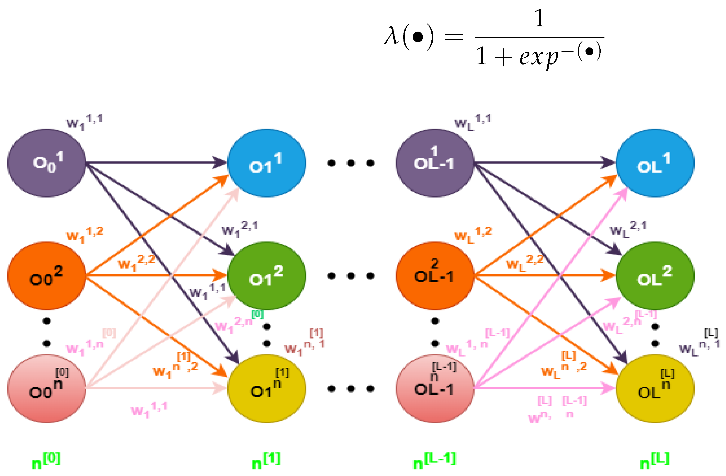
2.4. A Multi-Layer Neural Network Architecture

In Figure 2, a common structure of an MLNN is depicted consisting of L layers where $o_0=\left[\begin{array}{cccc}{o}_0^1& o_0^2& \dots & o_0^{n^{\left[0\right]}}\end{array}\right]$ is input layer, $o_L=\left[\begin{array}{cccc}{o}_L^1& o_L^2& \dots & o_L^{n^{\left[L\right]}}\end{array}\right]$ is output layer, and $o_i=\left[\begin{array}{cccc}{o}_i^1& o_i^2& \dots & o_i^{n^{\left[1\right]}}\end{array}\right]$ is the hidden layer. $n^{\left[i\right]}$ are the units in the $i^{th}$ layer, for $i=1,2,\dots L$. Each layer $o_{1,\cdots L}$ is expressed in the following form:

$$o_i=\lambda \left(W_{p_i}{o}_{i-1}+b_{p_i}\right)$$

(13)

where $W_{p_i}$, and $b_{p_i}$ are the weights and bias values for the MLNN layers, and $\lambda (•)$ represents the sigmoid activation function:

$$\begin{array}{c}\hfill \lambda (•)={\displaystyle \frac{1}{1+ex{p}^{-(•)}}}\end{array}$$

3. Proposed Method

The overall control strategy is illustrated in Figure 3. In this work, we utilize a dual-loop control architecture to achieve the target x-y translation and altitude control of UAV system. The outer-loop tracks the x and y position by providing the desired roll ${\varphi }_d$ and pitch ${\theta }_d$ commands to the inner-loop, where the inner-loop tracks the altitude, ${\varphi }_d, {\theta }_d$, and ${\psi }_d$ inputs by generating control inputs $T_1, {\tau }_2, {\tau }_3$ and ${\tau }_4$.

3.1. Multi-Layer Neural Network-Based Luenberger Observer Design

This section proposes an adaptive MLNN-based Luenberger observer for the quadrotor system to estimate the unknown system states $p, q$, and r in the attitude dynamic system. The attitude dynamics of the quadrotor system, given in (11), can be written to the form

$$\begin{array}{}{\dot{x}}_p\left(t\right)=A_p{x}_p\left(t\right)+G_p(x_p,u_p,d_p)\\ y_p\left(t\right)=C_p{x}_p\left(t\right)\end{array}$$

(14)

where $x_p\left(t\right)=col(x_7,x_8,x_9,x_{10},x_{11},x_{12})\in {\mathbb{R}}^6$, $u_p\left(t\right)={({\tau }_2,{\tau }_3,{\tau }_4)}^T\in {\mathbb{R}}^3$, $d_p\left(t\right)={\mathsf{\Omega }}_r\in {\mathbb{R}}^1$ and $y_p\left(t\right)\in {\mathbb{R}}^3$ are the states, input, disturbance, and output vectors respectively. In (14), $A_p=\left[\begin{array}{cc}{0}_3& I_3\\ 0_3& 0_3\end{array}\right]$ denotes system matrix, $G_p(x_p,u_p,d_p)=col\left(x_{10}{x}_{11}\left({\displaystyle \frac{I_{p_y}-I_{p_z}}{I_{p_x}}}\right)-{\displaystyle \frac{I_{p_r}}{I_{p_x}}}{x}_{10}{\mathsf{\Omega }}_r+{\displaystyle \frac{{\tau }_{\varphi }}{I_{p_x}}},x_8{x}_{12}\left({\displaystyle \frac{I_{p_z}-I_{p_x}}{I_{p_y}}}\right)-{\displaystyle \frac{I_{p_r}}{I_{p_y}}}{x}_8{\mathsf{\Omega }}_r+{\displaystyle \frac{{\tau }_{\theta }}{I_{p_y}}},x_8{x}_{10}\left({\displaystyle \frac{I_{p_x}-I_{p_y}}{I_{p_z}}}\right)+{\displaystyle \frac{{\tau }_{\psi }}{I_{p_z}}}\right)$ represents a nonlinear function contain unknown states which is to be estimated by the MLNN observer and $C_p=\left[\begin{array}{cc}{I}_3& 0_{3\times 3}\end{array}\right]$ denotes output matrix respectively. By following the results of Kolmogorov theorem, a non-linear function $G_p(x,u,d)$ is described in terms of activation function and ideal weights [37]:

$$\begin{array}{cc}\hfill G_p(x_p,u_p,d_p)& \hfill =W_L{\lambda }^0(W_{p_{L-1}},\dots W_{p_1},b_{p_{L-1}},\dots b_{p_1},o_0)+b_{p_L}+\aleph \left(x_p\right)\hfill \end{array}$$

(15)

where $\aleph \left(x_p\right)$ is an neural network approximation error satisfying $∥\aleph \left(x_p\right))∥\le {\aleph }_N$, where ${\aleph }_N$ is a positive number. An assumptions considered for designing the observer-based controller is that since the pair $(A_p,C_p)$ is observable (rank(obsv($A_p,C_p$)) = 6), the proposed NN-based Luenberger observer structure for attitude dynamic system (11) is given as [37]:

$$\begin{array}{cc}\hfill {\dot{\widehat{x}}}_p\left(t\right)& =A_p{\widehat{x}}_p\left(t\right)+{\mathbb{L}}_M\left(y_p\left(t\right)-{\widehat{y}}_p\left(t\right)\right)+{\widehat{G}}_p({\widehat{x}}_p,u_p,d_p)\hfill \\ \hfill {\widehat{G}}_p({\widehat{x}}_p,u_p,d_p)& ={\widehat{W}}_{p_L}{\lambda }^0\left({\widehat{W}}_{p_{L-1}},\cdots {\widehat{W}}_{p_1},{\widehat{b}}_{p_{L-1}},\cdots ,{\widehat{b}}_{p_1},{\widehat{o}}_0\right)+{\widehat{b}}_{p_L}\hfill \\ \hfill {\widehat{y}}_p\left(t\right)& =C_p{\widehat{x}}_p\left(t\right)\hfill \end{array}$$

(16)

where ${\widehat{x}}_p\left(t\right)$ represents the estimate of $x_p\left(t\right)$, ${\widehat{y}}_p\left(t\right)$ denote the estimated output, ${\mathbb{L}}_M\in {\mathbb{R}}^{6\times 3}$ represents the observer gain and ${\widehat{G}}_p({\widehat{x}}_p,u_p,d_p)$ is the unknown function to be estimated by the MLNN observer, whereas ${\widehat{W}}_{p_i}$ and ${\widehat{b}}_{p_i}$ define the NN-based learned weight matrices and bias vectors respectively shown in Figure 2. The error is $e_p\left(t\right)=x_p\left(t\right)-{\widehat{x}}_p\left(t\right)$, and its derivative ${\dot{e}}_p\left(t\right)$ after substituting (11) and (16) and adding and subtracting the term $\left[{\widehat{W}}_{p_L}{\lambda }^0\left({\widehat{W}}_{p_{L-1}},\cdots {\widehat{W}}_{p_1},{\widehat{b}}_{p_{L-1}},\cdots ,{\widehat{b}}_{p_1},{\widehat{o}}_0\right)\right]$ is obtained as

$$\begin{array}{cc}\hfill {\dot{e}}_p\left(t\right)=& \hfill H_p{e}_p\left(t\right)+e_{p_{b_L}}+\mathsf{{\rm Y}}\left(t\right)+\left[e_{w_{p_L}}{\lambda }^0\left({\widehat{W}}_{p_{L-1}},\cdots {\widehat{W}}_{p_1},{\widehat{b}}_{p_{L-1}},\cdots {\widehat{b}}_1,{\widehat{o}}_0\right)\right]\hfill \end{array}$$

(17)

where $e_{W_{p_L}}=W_{p_L-{\widehat{W}}_{p_L}},e_{p_{b_L}}=b_{p_L}-{\widehat{b}}_{p_L},H_p=A_p-{\mathbb{L}}_M{C}_p$ and $\mathsf{{\rm Y}}\left(t\right)$ denotes a bounded disturbance which ensures $∥\mathsf{{\rm Y}}∥\le \overline{\mathsf{{\rm Y}}}$, for a positive constant $\overline{\mathsf{{\rm Y}}}$, given as:

$\mathsf{{\rm Y}}\left(t\right)=W_{p_L}\left[{\lambda }^0\left(W_{p_{L-1}},\cdots ,W_{p_1},b_{p_{L-1}},\cdots b_{p_1},o_0\right)-{\lambda }^0\left({\widehat{W}}_{p_{L-1}},\cdots {\widehat{W}}_{p_1},{\widehat{b}}_{p_{L-1}},\cdots {\widehat{b}}_{p_1},{\widehat{o}}_0\right)\right]+$$\aleph \left(x_p\right)$. This study utilizes the following cost function.

$$\begin{array}{c}\hfill {\chi }_p={\displaystyle \frac{1}{2}}{e}_y^T{e}_y\end{array}$$

(18)

By employing the chain rule on (18) we get:

$$\begin{array}{c}\hfill {\displaystyle \frac{𝜕{\chi }_p}{𝜕{\widehat{W}}_{p_i}}}=diag{\left({\displaystyle \frac{𝜕C_p}{𝜕{\widehat{o}}_i}}\right)}^T{\displaystyle \frac{𝜕{\widehat{o}}_i}{𝜕{\widehat{o}}_i}}\end{array}$$

(19)

where ${\displaystyle \frac{𝜕{\chi }_p}{𝜕{\widehat{o}}_i}}={\displaystyle \frac{𝜕{\chi }_p}{𝜕e_y}}{\displaystyle \frac{𝜕e_y}{𝜕e_p}}{\displaystyle \frac{𝜕e_p}{𝜕{\widehat{o}}_L}}{\displaystyle \frac{𝜕{\widehat{o}}_L}{𝜕{\widehat{o}}_{L-1}}}{\displaystyle \frac{𝜕{\widehat{o}}_{L-1}}{𝜕{\widehat{o}}_{L-2}}}\dots {\displaystyle \frac{𝜕{\widehat{o}}_{i+1}}{𝜕{\widehat{o}}_i}}$, ${\displaystyle \frac{𝜕{\chi }_p}{𝜕e_y}}=e_y^T,{\displaystyle \frac{𝜕e_y}{𝜕e_p}}=C_p$ and ${\displaystyle \frac{𝜕e_p}{𝜕{\widehat{o}}_L}}=H_p^{-1}.$ For $e_y\left(t\right)=C_p{e}_p\left(t\right)$, after putting ${\displaystyle \frac{𝜕{\chi }_p}{𝜕e_y}}$,${\displaystyle \frac{𝜕e_y}{𝜕e_p}}$,${\displaystyle \frac{𝜕e_p}{𝜕{\widehat{o}}_L}}$ in (19), we obtain:

$$\begin{array}{c}\hfill {\displaystyle \frac{𝜕{\chi }_p}{𝜕{\widehat{W}}_{p_i}}}=diag{\left(e_p^T{C}_p^T{C}_p{H}_p^{-1}{\displaystyle \frac{𝜕{\widehat{o}}_L}{𝜕{\widehat{o}}_{L-1}}}{\displaystyle \frac{𝜕{\widehat{o}}_{L-1}}{𝜕{\widehat{o}}_{L-2}}}{\displaystyle \frac{𝜕{\widehat{o}}_{i+1}}{𝜕{\widehat{o}}_i}}\right)}^T{\displaystyle \frac{𝜕{\widehat{o}}_i}{𝜕{\widehat{W}}_{p_i}}}\end{array}$$

(20)

where

$$\begin{array}{cc}\hfill {\displaystyle \frac{𝜕{\widehat{o}}_L}{𝜕{\widehat{o}}_{L-1}}}& ={\widehat{W}}_{p_L}\hfill \\ \hfill {\displaystyle \frac{𝜕{\widehat{o}}_i}{𝜕{\widehat{W}}_{p_i}}}& ={\lambda }^{\prime }\left({\widehat{W}}_{p-i}{\widehat{o}}_{i-1}+{\widehat{b}}_{p_i}\right){\widehat{o}}_{i-1}^T\hfill \end{array}$$

3.2. Multi-Layer Neural Network Weight Update Law

This work employs a weight-tuning strategy that combines a modified back-propagation algorithm with gradient scaling, as detailed in references [34,37].

$$\begin{array}{cc}\hfill {\dot{\widehat{W}}}_{p_i}=& {\displaystyle \frac{-{\vartheta }_i}{{\prod }_{j=i+1}^{L-1}\parallel {\widehat{W}}_{p_j}+\varsigma \parallel }}{\displaystyle \frac{𝜕{\chi }_p}{𝜕{\widehat{W}}_{p_i}}}-\mathsf{{\rm Y}}\parallel e_p\parallel {\widehat{W}}_{p_i}\hfill \\ \hfill {\dot{\widehat{b}}}_{p_i}=& {\displaystyle \frac{-{\mu }_i\parallel {\widehat{b}}_{p_L}\parallel }{{\prod }_{j=i+1}^L\parallel {\widehat{W}}_{p_j}+\varsigma \parallel }}{\displaystyle \frac{𝜕{\chi }_p}{𝜕{\widehat{b}}_{p_i}}}-\mathsf{{\rm Y}}\parallel e\parallel {\widehat{b}}_{j_i}\hfill \end{array}$$

(21)

where ${\vartheta }_{i\cdots L}$, and ${\mu }_{i\cdots L}$ represent the learning rates, while $\mathsf{{\rm Y}}$ is a positive constant. Inserting (20) in (21):

$$\begin{array}{cc}\hfill {\dot{\widehat{W}}}_{p_i}& ={\displaystyle \frac{-{\vartheta }_i}{{\prod }_{j=i+1}^{L-1}\parallel {\widehat{W}}_{p_j}+\varsigma \parallel }}diag({{\displaystyle \frac{𝜕{\chi }_p}{𝜕{\widehat{o}}_i}}}^T)\acute{\lambda }(W_{p_i}{o}_{i-1}+b_{p_i})o_{i-1}^T\hfill \\ & -\mathsf{{\rm Y}}\parallel e_p\parallel {\widehat{W}}_{p_i}\hfill \\ \hfill {\dot{\widehat{b}}}_{p_i}& ={\displaystyle \frac{-{\mu }_i\parallel {\widehat{b}}_{p_L}}{{\prod }_{j=i+1}^L\parallel {\widehat{W}}_{p_j}+\varsigma \parallel }}diag({{\displaystyle \frac{𝜕{\chi }_p}{𝜕{\widehat{o}}_{p_i}}}}^T)\acute{\lambda }(W_{p_{L-1}}{o}_{L-2}+b_{p_{L-1}})\hfill \\ & -\mathsf{{\rm Y}}\parallel e_p\parallel {\widehat{b}}_{p_i}\hfill \end{array}$$

(22)

where $\varsigma$ is chosen to be smaller. Consequently, the output layer’s adaptive law is derived as

$$\begin{array}{c}\hfill {\dot{\widehat{W}}}_{p_L}=diag{\left(e_p^T{T}_L\right)}^T{o}_{L-1}^T-\mathsf{{\rm Y}}\parallel e_p\parallel {\widehat{W}}_{p_L}\end{array}$$

(23)

Theorem 1.

Suppose $P_o$ is a positive definite, while $Q_o$ is another matrix, satisfying the equality:

$$H_p^T{P}_o+P_o{H}_p=-Q_o$$

(24)

then the error (17) remains within bounds if the subsequent condition is fulfilled:

$$\begin{array}{c}\hfill ∥e_p∥>{\displaystyle \frac{2\left(\genfrac{}{}{0pt}{}{∥\mathbb{P}∥{\lambda }^{\prime }+{\sum }_{i=1}^{L-1}\left(\frac{\mathsf{{\rm Y}}}{L-1}-{\mathsf{{\rm Y}}}_i^2\right){\mathsf{{\rm Y}}}_{2i}^2+{\sum }_{i=1}^{L-1}\left(\mathsf{{\rm Y}}-1\right){\mathsf{{\rm Y}}}_{3i}^2}{+{\sum }_{i=1}^{L-1}\left(\frac{\mathsf{{\rm Y}}}{L-1}-{\varrho }_{2i}^2\right)-{\sum }_{i=1}^{L-1}\left(\mathsf{{\rm Y}}-1\right){\varrho }_{3i}^2}\right)}{{\zeta }_{min}\left(\mathbb{Q}\right)}}\end{array}$$

(25)

Proof. 

To establish the proposed MLNN-observer’s stability, we extend the single-layer neural network architecture [34,37] to a multi-layer with the modified back-propagation weight update rule. In Appendix A, the proof of this theorem is provided. □

Remark 2.

This study develops an MLNN-based observer (16) to predict the internal states of the quadrotor, such as angular rates. The observer error dynamics (17) is stable if the conditions given in (24)–(25) are satisfied.

3.3. NDI Based Fast Terminal SMC Law

This section proposes an NDI-based fast terminal SMC law to attain the position and attitude-tracking control of a UAV. Since the attitude dynamic system depends on the estimated states obtained from the MLNN observer, we first consider the detailed formulation of the attitude dynamic control law. Meanwhile, the other control laws are designed along similar lines. The proposed control law is designed in two steps. First, the NDI controller is developed to cancel the nonlinearities without considering the disturbance effect. Then, the adaptive fast terminal SMC law is integrated, which provides robustness against disturbance/uncertainty. Therefore, NDI-based fast terminal SMC control law can be written in the following form:

$$u_p\left(t\right)=u_{p_n}\left(t\right)+u_{p_l}\left(t\right)$$

(26)

where $u_{p_l}\left(t\right)$ is the NDI component of the control law without considering disturbances, and $u_{p_n}\left(t\right)$ denotes the fast terminal SMC component, which is the adaptive part to deal with disturbances. According to (11), the attitude dynamics of the quadrotor are affine in input. Since, the attitude angle states are available at the output, the output dynamics of the attitude subsystem (14) can also be written into the form

$$\begin{array}{c}\hfill {\dot{y}}_p\left(t\right)=C_p{A}_p{x}_p+C_p{B}_p{u}_p+C_p{G}_p(x_p,t)+C_p{D}_p{d}_p\left(t\right)\end{array}$$

(27)

where $B_p={\left[0_{3\times 3}diag(1/I_{p_x},1/I_{p_y},1/I_{p_z})\right]}^T$, $C_p=\left[I_{3\times 3}{0}_{3\times 3}\right]$, $D_p=col(0_{3\times 3},{\displaystyle \frac{I_{p_r}}{I_{p_x}}}{x}_{10},{\displaystyle \frac{I_{p_r}}{I_{p_y}}}{x}_8,0)$ and $d_p\left(t\right)={\mathsf{\Omega }}_r.$

3.3.1. NDI Control Law

The attitude dynamics of the quadrotor (12), after neglecting the effect of disturbance/uncertainty, can be written as

$$\begin{array}{c}\hfill {\dot{y}}_p\left(t\right)=C_p{A}_p{x}_p+C_p{B}_p{u}_p+C_p{G}_p(x_p,t)\end{array}$$

(28)

Define the desired attitude states $y_{p_d}\in {[{\varphi }_d,{\theta }_d,{\psi }_d]}^T$ and its derivatives ${\dot{y}}_d$. The control input is then designed as

$$u_{p_n}=-{\left(C_p{B}_p\right)}^{-1}(C_p{A}_p{x}_p+C_p{G}_p({\widehat{x}}_p,t)+{\dot{y}}_d)$$

(29)

where ${\widehat{x}}_p$ denotes the estimated state acquired from the MLNN observer and ${\dot{y}}_d$ denotes the desired dynamics defined as

$${\dot{y}}_d=k_p{e}_y+k_i\int e_{y}dt$$

(30)

where $e_y=y_d-y$ denotes tracking error, $k_p=diag(k_{p_{\varphi }},k_{p_{\theta }},k_{p_{\psi }})$ and $k_i=diag(k_{i_{\varphi }},k_{i_{\theta }},k_{i_{\psi }})$ are NDI controller parameter that determine the desired attitude dynamics.

3.3.2. Fast Terminal SMC Law

The next step is integrating fast terminal SMC law to enhance system robustness. Therefore, the fast terminal SMC law $u_{p_S}\left(t\right)$ is defined as

$$u_{p_s}\left(t\right)=-{\mathcal{K}}_{f}sign\left(s_p\right)-{\eta }_f{s}_p^{{\beta }_f}$$

(31)

where ${\mathcal{K}}_f=diag({\kappa }_{f_{\varphi }},{\kappa }_{f_{\theta }},{\kappa }_{f_{\psi }})$, ${\eta }_f=diag({\eta }_{f_{\varphi }},{\eta }_{f_{\theta }},{\eta }_{f_{\psi }})$ are the sliding gains and $0<{\beta }_f<1$ is fast terminal SMC design parameters, $s_p\left(t\right)\in {\Re }^{3\times 1}$ denotes the sliding surface defined as

$$s_p\left(t\right)=e_y\left(t\right)+{\lambda }_f{e}_y^{{\alpha }_f}\left(t\right)$$

(32)

where ${\lambda }_f>0$ and $0<{\alpha }_f<1$ are design parameters.

Remark 3.

The parameters ${\lambda }_f$ and ${\eta }_f$ of fast terminal SMC law play crucial roles in determining the effectiveness and robustness of the controller design. The parameter ${\lambda }_f$ influences on convergence rate and transient response while ${\eta }_f$ impacts robustness and steady-state error. Achieving an optimal balance between control effort, robustness and swift response in the control system requires precise tuning of these parameters.

3.4. The Stability Analysis

Substitute the control law (26)–(31) into the system dynamics (27), we get

$${\dot{e}}_y\left(t\right)=-{\mathcal{K}}_{f}sign\left(s_p\right)-{\eta }_f{s}_p^{{\beta }_f}+{\dot{y}}_d+C_p(G_p(x_p,t)-{\widehat{G}}_p({\widehat{x}}_p,t))+C_p{D}_p{d}_p\left(t\right)$$

(33)

The derivative of switching function (32) after substituting the (33) is obtained as

$$\begin{array}{c}\hfill {\dot{s}}_p=\left(-{\mathcal{K}}_{f}sign\left(s_p\right)-{\eta }_f{s}_p^{{\beta }_f}+{\dot{y}}_d+C_p(G_p(x_p,t)-{\widehat{G}}_p({\widehat{x}}_p,t))+C_p{D}_p{d}_p\left(t\right)\right)\\ \hfill (1+{\lambda }_f{\alpha }_f{e}_y^{{\alpha }_f-1})\end{array}$$

(34)

To prove system stability, define the Lyapunov function as

$$V_p={\displaystyle \frac{1}{2}}{s}_p^T\left(t\right)s_p\left(t\right)$$

(35)

Taking the time derivative of Lyapunov function and substitute (34), we get

$$\begin{array}{cc}\hfill {\dot{V}}_p=& s_p^T\left(-{\mathcal{K}}_{f}sign\left(s_p\right)-{\eta }_f{s}_p^{{\beta }_f}+{\dot{y}}_d+C_p(G_p(x_p,t)-{\widehat{G}}_p({\widehat{x}}_p,t))+C_p{D}_p{d}_p\left(t\right)\right)\hfill \\ & (1+{\lambda }_f{\alpha }_f{e}_y^{{\alpha }_f-1})\hfill \end{array}$$

(36)

Assuming the nonlinear function $G_p(x_p,t)$ satisfies the Lipschitz condition than we can write [49,50]

$$C_p(G_p(x_p,t)-{\widehat{G}}_p({\widehat{x}}_p,t))\le L_f\parallel e_y\left(t\right)\parallel$$

(37)

where $L_f$ is Lipschitz constant. Utilizing (37), we get

$${\dot{V}}_p\le \parallel s_p^T\parallel \left(-{\mathcal{K}}_f-{\eta }_f\parallel s_p^{{\beta }_f}\parallel +\parallel {\dot{y}}_d\parallel +L_f\parallel e_y\left(t\right)\parallel +\parallel C_p{D}_p{d}_p\left(t\right)\parallel \right)(1+{\lambda }_f{\alpha }_f\parallel e_y^{{\alpha }_f-1}\parallel )$$

(38)

To ensure ${\dot{V}}_p<0$, the following conditions on $K_f$ and ${\eta }_f$ must be satisfied

$$K_f\ge {\displaystyle \frac{\parallel {\dot{y}}_d\parallel +L_f\parallel e_y\left(t\right)\parallel +\parallel C_p{D}_p{d}_p\left(t\right)\parallel }{1+{\lambda }_f{\alpha }_f\parallel e_y^{{\alpha }_f-1}\parallel }},{\eta }_f\ge 0$$

(39)

Hence, ${\dot{V}}_p<0$. This ensures the convergence of the sliding surface $s_p\left(t\right)$ to zero, thereby stabilizing the system despite disturbances.

Remark 4.

The final control law (26) is derived by incorporating the NDI control law (29) and fast terminal SMC law (31), provided that the sliding gains are chosen according to (39), and the estimated state information is obtained from (16).

The outer loop position control is achieved by generating the desired roll ${\varphi }_d$ and pitch commands ${\theta }_d$ commands to the inner loop subsystem. The control laws for outer loop is designed in similar way as

$$\begin{array}{c}\hfill u_x={\displaystyle \frac{m}{T_1}}({\dot{x}}_d-k_{x}sign\left(s_x\right)-{\eta }_x{s}_x^{{\beta }_x})\\ \hfill u_y={\displaystyle \frac{m}{T_1}}({\dot{y}}_d-k_{y}sign\left(s_y\right)-{\eta }_y{s}_y^{{\beta }_y})\\ \hfill T={\displaystyle \frac{m}{C{x}_{7}C{x}_9}}({\dot{z}}_d-k_{z}sign\left(s_z\right)-{\eta }_z{s}_z^{{\beta }_z})\end{array}$$

(40)

where $x_d, y_d$ and $z_d$ are the desired $x, y$ and z positions, $k_x, k_y, k_z$ and ${\eta }_x, {\eta }_y, {\eta }_z$ are the sliding gains, and $s_x, s_y, s_z$ are the sliding surfaces defined as:

$$\begin{array}{c}\hfill s_x=e_x+{\lambda }_{f_x}{e}_x^{{\alpha }_{f_x}}\left(t\right)\\ \hfill s_y=e_y+{\lambda }_{f_y}{e}_y^{{\alpha }_{f_y}}\left(t\right)\\ \hfill s_z=e_z+{\lambda }_{f_z}{e}_z^{{\alpha }_{f_z}}\left(t\right)\end{array}$$

here $e_x=x_d-x, e_y=y_d-y, e_z=z_d-z$. ${\varphi }_d$ and ${\theta }_d$ are the desired roll and pitch commands calculated as

$$\begin{array}{c}\hfill {\varphi }_d=si{n}^{-1}\left(u_{x}sin{\psi }_d-u_{y}cos{\psi }_d\right)\\ \hfill {\theta }_d=si{n}^{-1}\left({\displaystyle \frac{u_{x}sin{\psi }_d-u_{y}cos{\psi }_d}{cos{\varphi }_d}}\right)\end{array}$$

(41)

4. Parameter Setting and Results

This section discusses the efficacy of the scheme designed in the previous section by testing it on a nonlinear model of the quadrotor system. To validate the simulation results, HIL simulations are performed using Pixhawk 6X flight controller. Then, the experiments are conducted on real-time hardware setup of F450 in a constrained indoor environment.

4.1. Parameter Settings

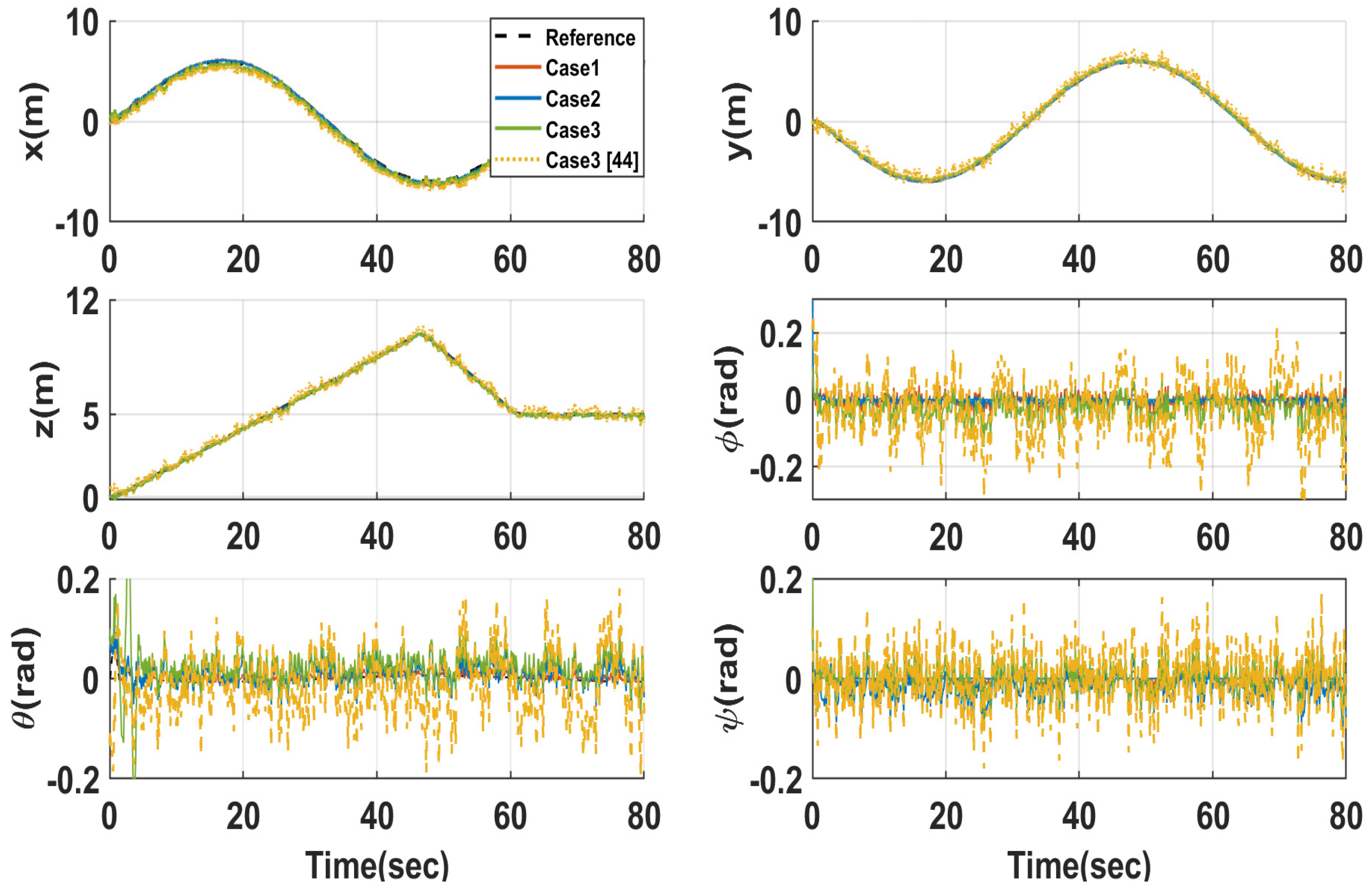
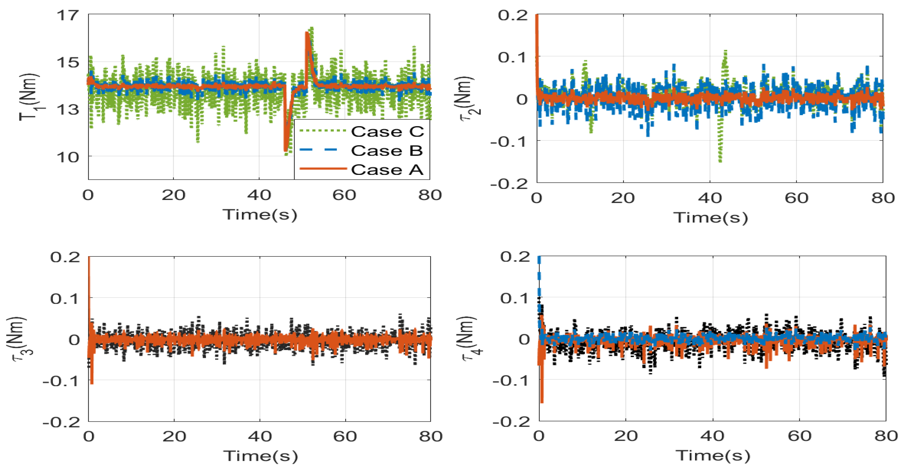
The MLNN observer is trained using data generated from the quadrotor UAV model. The inputs to the MLNN are $\varphi , \theta , \psi$, while the outputs are $\widehat{p}, \widehat{q}$, and $\widehat{r}$, as depicted in Figure 4. The neural network undergoes training using input-output data to approximate states closely resembling the actual ones. The neural network is structured with four hidden layers, each comprising 10, 12, 12, and 20 neurons, respectively, all employing a sigmoid activation function. The network’s initial weights and bias terms are set with small random values, and these weights are subsequently refined and adjusted using the modified back-propagation algorithm. During training, the input data is processed through the network’s layers, and the difference between predicted and actual outputs is calculated. This error is then propagated backward through the network to compute gradients, which guide the adjustment of weights and biases via a modified backpropagation algorithm. The network undergoes multiple iterations or epochs of this process, refining its parameters to minimize the error and improve predictive accuracy so that the estimated states closely resemble the actual ones, thus improving the network’s ability to make accurate predictions. After training, the trained MLNN model is placed in run-time simulations to estimate states and evaluate the observer’s performance. The controller and observer gains are given in

Table 2. Parameter values of controller/observer.

Gain	$k_{p_{\varphi }}$	$k_{p_{\theta }}$	$k_{p_{\psi }}$	$k_{p_x}$	$k_{p_y}$	$k_{p_z}$
Value	5	5	2.5	10	10	5
Gain	$k_{i_{\varphi }}$	$k_{i_{\theta }}$	$k_{i_{\psi }}$	$k_{i_x}$	$k_{i_y}$	$k_{i_z}$
Value	3.75	3.75	2.5	3.5	3.25	5
Gain	${\kappa }_{f_{\varphi }}$	${\kappa }_{f_{\theta }}$	${\kappa }_{f_{\psi }}$	${\kappa }_{f_x}$	${\kappa }_{f_y}$	${\kappa }_{f_z}$
Value	3	3	1.5	2.5	2.5	4
Gain	${\eta }_{f_{\varphi }}$	${\eta }_{f_{\theta }}$	${\eta }_{f_{\psi }}$	${\eta }_{f_x}$	${\eta }_{f_y}$	${\kappa }_{f_z}$
Value	0.5	0.5	1	0.25	0.25	0.01
Gain	$\gamma$	$\beta$	$\mathsf{{\rm Y}}$	${\lambda }_{f_x}$	${\lambda }_{f_y}$	${\lambda }_{f_z}$
Value	238	205	0.008	0.08	0.08	0.05

.

4.2. Results

This subsection initially evaluates the performance of the suggested scheme with numerical simulations on the nonlinear model (1)–(9). Then, HIL simulations are performed using Pixhawk 6X autopilot. Finally, real tests are performed on the F450 quadrotor system mounted on the frame for safe indoor environment.

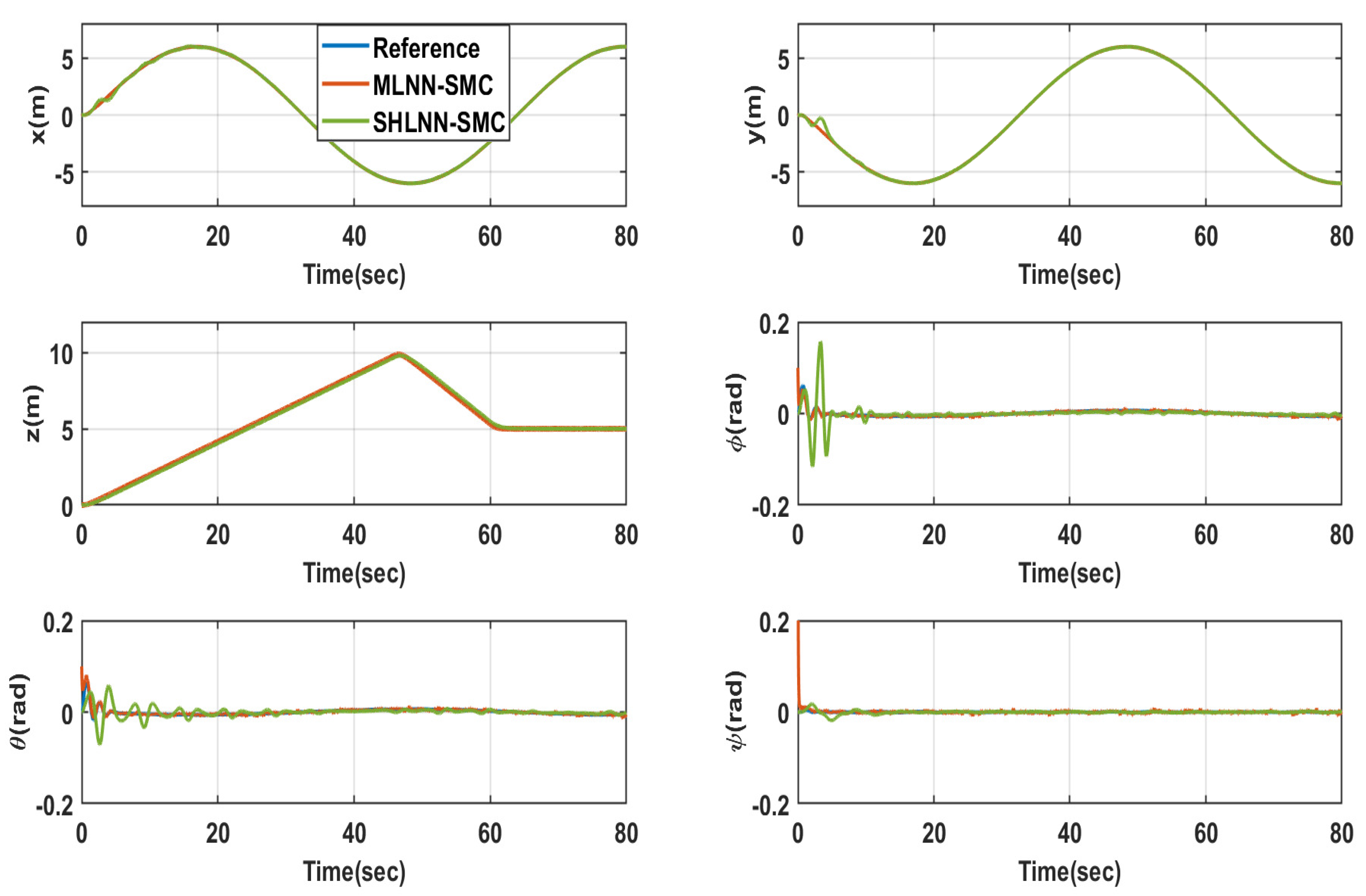
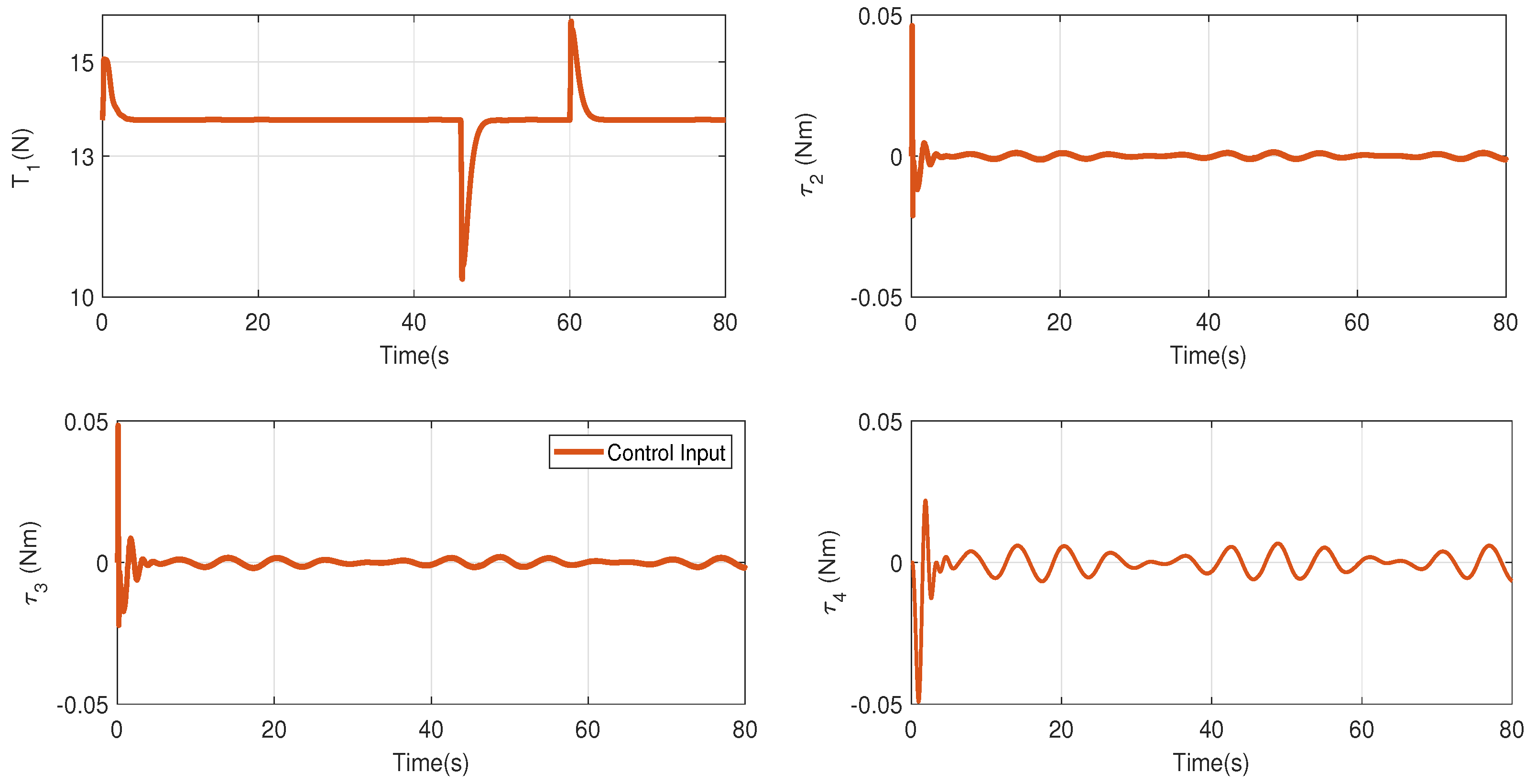
4.3. Numerical Simulations

In this subsection, the effectiveness of the proposed method is tested on a nonlinear model of aircraft given in (1)–(6). A sine and cosine function of amplitude 6 m is applied to desired x and y positions. The desired z position ramps up from 0 to 10 m over 50 s, reaching a height of 5 m at 60 s, and remains constant thereafter. Our trajectory represents a gradually ascending circular path, which is commonly used in realistic UAV applications to generate circular ascending flight patterns [51,52,53]. This data is used to train the neural network. The proposed method is tested by considering two different conditions; the first one is nominal scenarios, and the other considers the effect of disturbance and parameter variations. To evaluate the performance of the proposed scheme subject to parameter variation, a performance index is defined as

$$e_{MS{E}_i}={\displaystyle \frac{1}{t_f-t_i}}{\int }_{t_i}^{t_f}{e}_i{\left(t\right)}^{2}dt$$

where $e_{MS{E}_i}$ represents the mean square error and $e_i$ is the error between $i^{th}$ desired and state estimated by the proposed scheme.

4.3.1. Nominal Condition

In this subsection, the simulations are conducted without incorporating noise or wind gusts into the plant dynamics. The results depicted in Figure 5 illustrate the state tracking results of the proposed observer-based controller under nominal conditions. The comparison is made with the adaptive neural network extended state observer (ANNESO) employing a single hidden layer neural network architecture given in [39]. The simulation results showcase outstanding tracking performance for the $x, y$, and z positions and the attitude angles for the proposed scheme. The plots of control input are depicted in Figure 6, and the mean square error calculation in the nominal condition is given in

Table 3. Comaprison of mean square error values for nominal case.

Parameters	Proposed Scheme	[39]
$e_{MS{E}_x}$	3.3 × ${10}^{-6}$	6.2 × ${10}^{-6}$
$e_{MS{E}_y}$	2.5 × ${10}^{-6}$	4.3 × ${10}^{-6}$
$e_{MS{E}_z}$	2.01 × ${10}^{-6}$	3.3 × ${10}^{-6}$
$e_{MS{E}_{\varphi }}$	1.3 × ${10}^{-5}$	3.9 × ${10}^{-5}$
$e_{MS{E}_{\theta }}$	2.13 × ${10}^{-5}$	4.4 × ${10}^{-5}$
$e_{MS{E}_{\psi }}$	3.4 × ${10}^{-5}$	5.1 × ${10}^{-5}$

.

4.3.2. Results with Noise, Disturbance and Parameter Variations

To validate the performance of the proposed MLNN observer-based control scheme, we presented three different cases for parameter variation ($5\%$, $10\%$, and $15\%)$ and wind-gust condition (mean velocity of 4 m/s, 6 m/s and 8 m/s), For each case, the noise with a variance of $0.02$ and zero mean values is added to the $p, q, r$ and z states. Wind gusts effect using the Dryden wind gust model [54] are added into the non-linear plant equations.

Figure 7 and Figure 8 showcases the tracking of states and control input results respectively under noise, wind gust, and parameter variation across cases A, B, and C, respectively. Noise and external aerodynamic effects during flight can lead to variations in the parameters of UAVs, including mass, moments of inertia along the $x, y,$ and z axes, drag forces, and coefficient of thrust. The adaptive gains of the MLNN observer mitigate the impact of such factors, facilitating the estimation of trajectories that closely resemble the reference trajectories. Despite parameter variations in Case B and C causing slight deviations from the desired trajectory, the proposed adaptive MLNN effectively learns and rejects the nonlinearities. Additionally, the NDI-based Fast Terminal SMC incorporates robustness to further enhance performance. The comparison of the proposed scheme is made with an existing work presented in [44]. The results are compared considering only worst case scenario of parameters variations and disturbance presented in Case C. These simulation plots indicate that the proposed scheme exhibits less deviation and noise impact due to its adaptive nature, compared to [44]. The MSE values for the Cases A, B, and C are provided in

Table 4. MSE values under noise, disturbance, and parameter variations.

Parameters	Case A	Case B	Case C	Case C [44]
$e_{MS{E}_x}$	2.5 × ${10}^{-5}$	6.1 × ${10}^{-5}$	3.1 × ${10}^{-4}$	4.9 × ${10}^{-3}$
$e_{MS{E}_y}$	1.63 × ${10}^{-5}$	5.7 × ${10}^{-5}$	2.4 × ${10}^{-4}$	3.8 × ${10}^{-3}$
$e_{MS{E}_z}$	1.1 × ${10}^{-5}$	2.9 × ${10}^{-5}$	2.1 × ${10}^{-4}$	8.3 × ${10}^{-3}$
$e_{MS{E}_{\varphi }}$	8.3 × ${10}^{-5}$	2.3 × ${10}^{-4}$	5.2 × ${10}^{-4}$	7.3 × ${10}^{-3}$
$e_{MS{E}_{\theta }}$	9.13 × ${10}^{-5}$	3.5 × ${10}^{-4}$	9.8 × ${10}^{-3}$	4.13 × ${10}^{-2}$
$e_{MS{E}_{\psi }}$	2.35 × ${10}^{-4}$	4.2 × ${10}^{-4}$	6.7 × ${10}^{-4}$	3.4 × ${10}^{-3}$

. Additionally, the MSE comparison between the proposed scheme and [44] for Case C is also provided which clearly shows that the MSE values of the proposed scheme are lower than those of the scheme suggested in [44] which ensure better tracking accuracy.

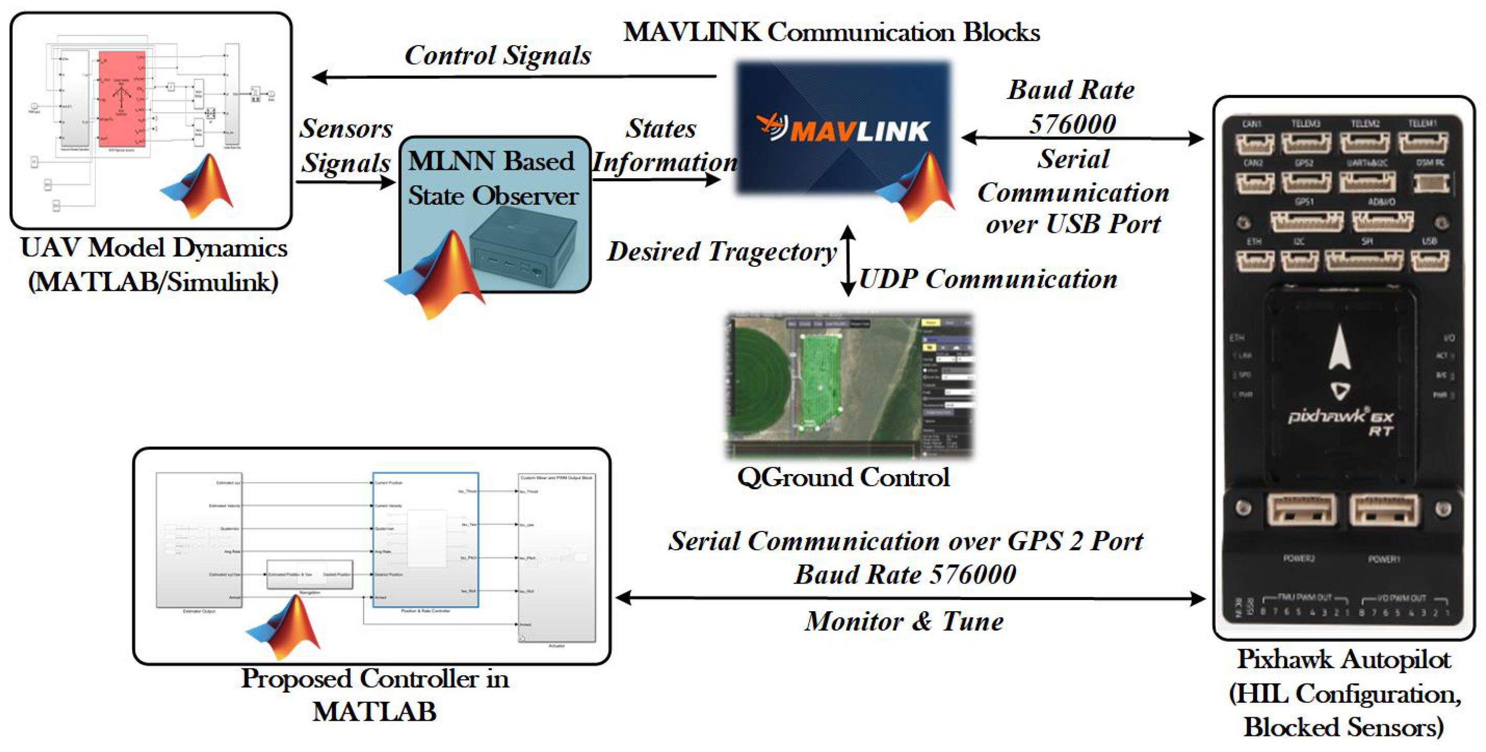
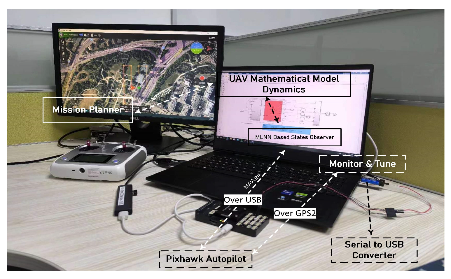
4.4. Hardware-in-the-Loop Simulations

In this section, we conducted HIL simulations utilizing the Pixhawk 6X flight controller to showcase the algorithm’s viability in practical scenarios. These simulations offer concrete proof of the effectiveness and applicability of our control algorithm during real-time UAV operations. The Pixhawk flight controller board is interfaced with the Mission Planner platform. These simulations aimed to validate the controller design implemented on the Pixhawk hardware board, incorporating UAV and MLNN observer dynamics within Simulink. Flight missions were programmed in QGroundControl (QGC), guiding the flight controller algorithm to follow the designated missions. The connection setup for HIL simulations is given in Figure 9, which illustrates the communication setup between MATLAB, Pixhawk, and QGround Control. The communication relies on the Mavlink protocol, recognized as the standard communication protocol for UAVs. In HIL architecture shown in Figure 10, the control algorithm operates on the Pixhawk 6X, while the computational dynamics of the UAV and observer dynamics are performed on a host computer. Simulink’s Monitor and Tune simulation tool is utilized for real-time logging and tuning of controller settings. The host computer computes dynamics, transmitting the data to the PX4 Autopilot via the USB port. The PX4 autopilot calculates thrust and torque based on the received data, establishes a hardware loop, and sends them back to the host. An additional serial port on the Pixhawk 6X is employed to establish communication between the PX4 Autopilot and Simulink for utilizing the monitor and tune tool. The altitude and attitude tracking results of the proposed scheme are showcased in Figure 11, while position tracking results are given in Figure 12. The results clearly demonstrate that the proposed MLNN observer-based NDI fast terminal SMC scheme closely follows the desired trajectories. The control inputs displayed in Figure 13 are bounded within a specific range.

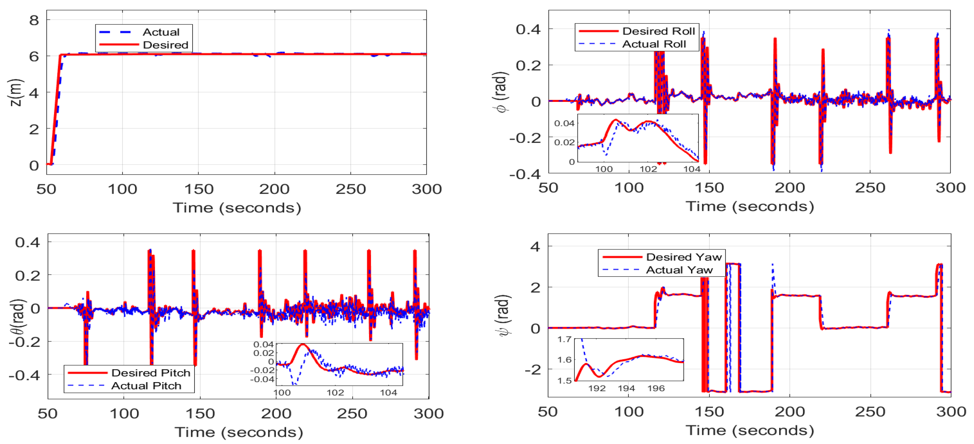
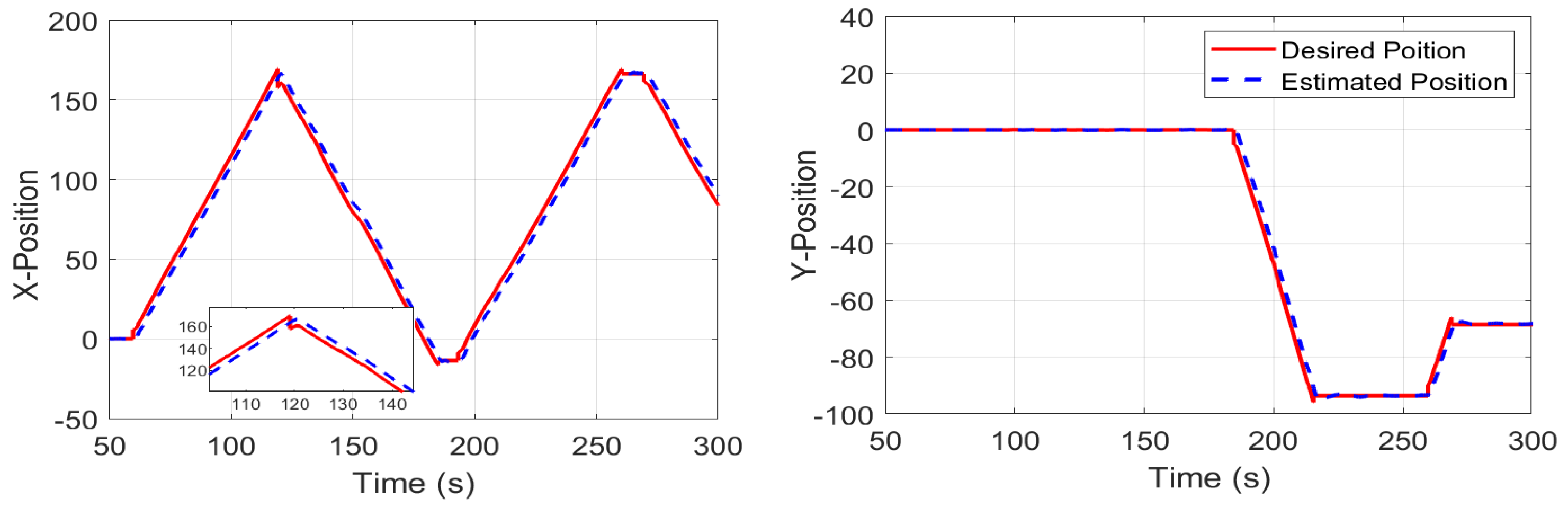
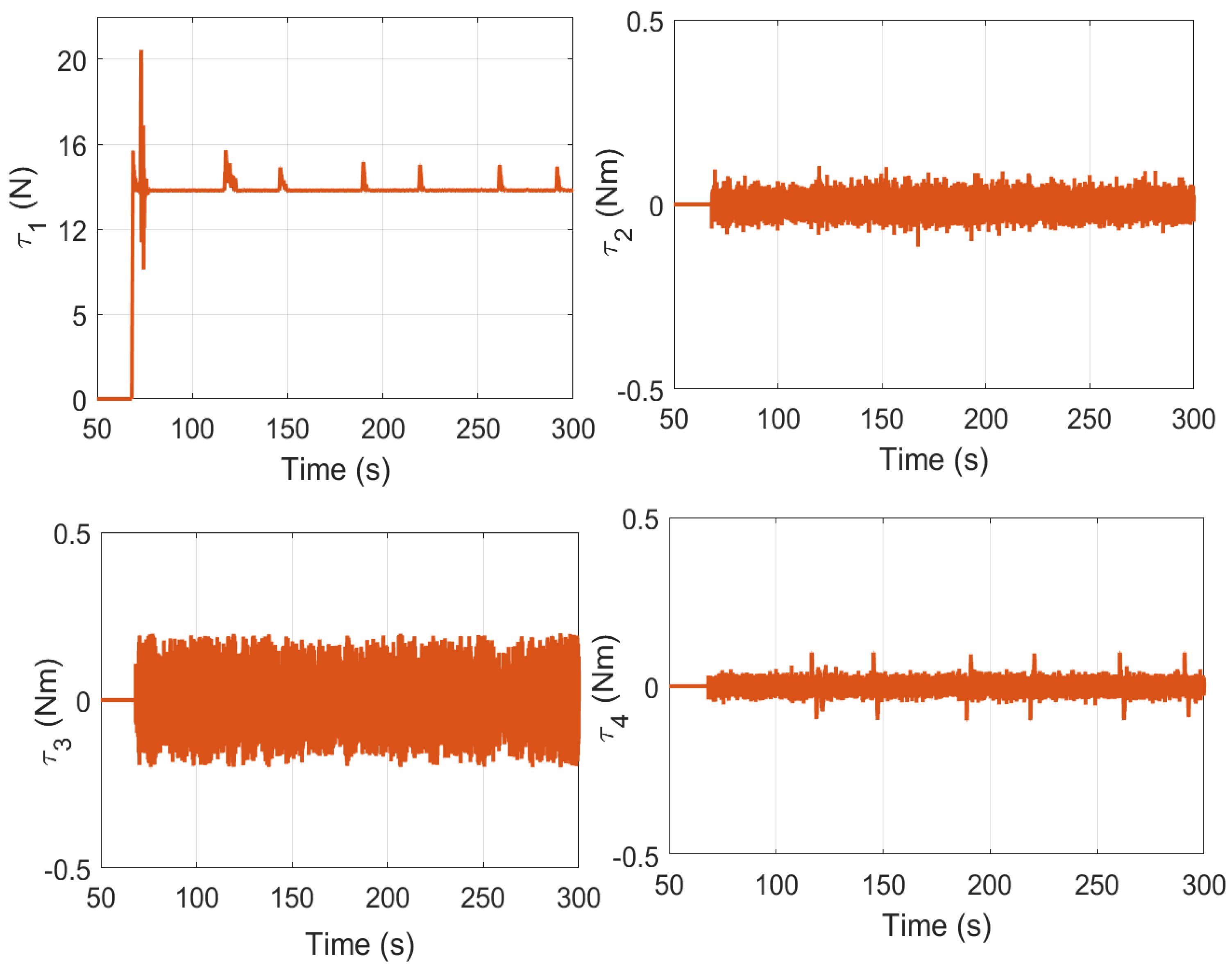
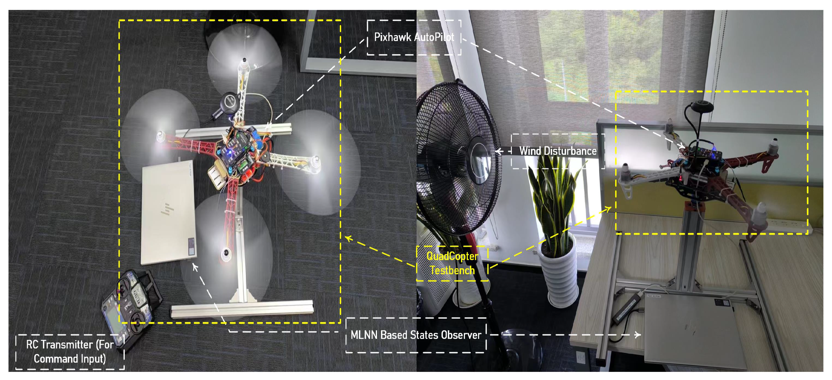
4.5. Experimental Results on Quadrotor Test-Rig

The real-time hardware setup comprises a F450 X-configuration quadrotor frame, Pixhawk 6X Autopilot, RC Transmitter and receiver (FS-i6) given in Figure 14. The propeller system includes 4 permanent magnet synchronous motors (PMSM) with KV-950 and 20A Esc, powered by a 5000 mAh Li-po battery with a low-battery tester. The experimental setup is mounted on a safety stand that is only capable of performing attitude tracking. The Pixhawk 6X is equipped with a comprehensive sensor suite for precise navigation and control. It includes three ICM-42688 IMUs, featuring balanced gyro technology for measuring linear acceleration and angular velocity which are essential for flight stabilization and smooth movement. The system also incorporates two barometers, the ICP20100 and BMP388, for accurate altitude measurement, and a BMM150 magnetometer to detect orientation relative to Earth’s magnetic field. These sensors work together to provide reliable flight data, enabling autonomous operations and real-time flight adjustments. The quadcopter is securely mounted on a safety aluminum stand with a spherical ball joint to ensure the safety of the environment and personnel during testing, allowing observation of three primary movements: roll, pitch, and yaw. The MLNN-based observer is simulated using a high-processing laptop, which communicates with the Pixhawk via a wired RS232 protocol. The control algorithm operates on the Pixhawk 6x, with all necessary hardware devices interfaced accordingly. The desired roll, pitch, and yaw commands are inputted to the quadrotor using the RC transmitter, while the RC receiver receives Pulse Position Modulation (PPM) commands from the transmitter and forwards them as reference signals to the autopilot. The Pixhawk autopilot executes the desired attitude commands based on the state inputs from the MLNN observer and sensors, generating thrust and torque commands in the form of Pulse Width Modulation (PWM) signals for the motors. The safety stand allowed us to capture real-time flight data without compromising the accuracy of the results. Thus, the data presented reflects practical flight behavior, despite the UAV being physically secured for safety reason. The attitude tracking results with wind disturbance are depicted in Figure 15, demonstrating commendable performance when implemented on a real F450 quadrotor.

5. Conclusions

This work proposes an adaptive MLNN-observer-based NDI fast terminal SMC scheme for quadrotor UAV. The adaptive MLNN-observer is based on a modified back-propagation algorithm that alleviates the impacts of wind disturbances, parameter uncertainties, and noise by learning the non-linearities in the data. A rigorous stability analysis is performed to guarantee the convergence of observer error dynamics. Then, NDI-based fast terminal SMC laws are designed with both inner and outer loops, which provide attitude and position tracking control while contributing towards additional robustness. To test the efficacy of the proposed approach, simulations are first performed in different operating conditions. To validate the numerical simulations, HIL simulations are conducted using Pixhawk 6X flight controller. Finally, the hardware test are performed in constraint indoor environment hardware-in-loop simulations using a real quadrotor F450 platform to validate the effectiveness of the proposed method. In future, the MLNN based observer will be extended to estimate both sensor and actuators fault and external disturbance and closed loop performance will be analyzed in the presence of sensor and actuator malfunctioning.

References

1. Wang, E.; Sun, J.; Liang, Y.; Zhou, B.; Jiang, F.; Zhu, Y. Modeling, Guidance, and Robust Cooperative Control of Two Quadrotors Carrying a “Y”-Shaped-Cable-Suspended Payload. Drones 2024, 8, 103. [Google Scholar] [CrossRef]
2. Hanif, A.S.; Han, X.; Yu, S.-H. Independent Control Spraying System for UAV-Based Precise Variable Sprayer: A Review. Drones 2022, 6, 383. [Google Scholar] [CrossRef]
3. Yang, T.S.; Yang, F.; Li, D. A New Autonomous Method of Drone Path Planning Based on Multiple Strategies for Avoiding Obstacles with High Speed and High Density. Drones 2024, 8, 205. [Google Scholar] [CrossRef]
4. Hu, Z.; Jin, X. Adaptive formation control architectures for a team of quadrotors with multiple performance and safety constraints. Int. J. Robust Nonlinear Control 2023, 33, 8183–8204. [Google Scholar] [CrossRef]
5. Zhao, W.; Liu, H.; Wang, B. Model-free attitude synchronization for multiple heterogeneous quadrotors via reinforcement learning. Int. J. Intell. Syst. 2021, 36, 2528–2547. [Google Scholar] [CrossRef]
6. Zhao, W.; Liu, H.; Lewis, F.L. Data-driven fault-tolerant control for attitude synchronization of nonlinear quadrotors. IEEE Trans. Autom. Control 2021, 66, 5584–5591. [Google Scholar] [CrossRef]
7. Xian, W.; Qi, Q.; Liu, W.; Liu, Y.; Li, D.; Wang, Y. Control of quadrotor robot via optimized nonlinear type-2 fuzzy fractional PID with fractional filter: Theory and experiment. Aerosp. Sci. Technol. 2024, 151, 109286. [Google Scholar] [CrossRef]
8. Zhang, X.; Li, H.; Zhu, G.; Zhang, Y.; Wang, C.; Wang, Y.; Su, C.-Y. Finite-Time Adaptive Quantized Control for Quadrotor Aerial Vehicle with Full States Constraints and Validation on QDrone Experimental Platform. Drones 2024, 8, 264. [Google Scholar] [CrossRef]
9. Lyu, X.; Zhou, J.; Gu, H.; Li, Z.; Shen, S.; Zhang, F. Disturbance Observer Based Hovering Control of Quadrotor Tail-Sitter VTOL UAVs Using H Synthesis. IEEE Robot. Autom. Lett. 2018, 3, 2910–2917. [Google Scholar] [CrossRef]
10. Castillo, A.; Sanz, R.; Garcia, P.; Qiu, W.; Wang, H.; Xu, C. Disturbance observer-based quadrotor attitude tracking control for aggressive maneuvers. Control Eng. Pract. 2019, 82, 14–23. [Google Scholar] [CrossRef]
11. El-Sousy, F.F.; Alattas, K.A.; Mofid, O.; Mobayen, S.; Asad, J.H.; Skruch, P.; Assawinchaichote, W. Non-singular finite time tracking control approach based on disturbance observers for perturbed quadrotor unmanned aerial vehicles. Sensors 2022, 22, 2785. [Google Scholar] [CrossRef]
12. Wang, J.; Alattas, K.A.; Bouteraa, Y.; Mofid, O.; Mobayen, S. Adaptive finite-time backstepping control tracker for quadrotor UAV with model uncertainty and external disturbance. Aerosp. Sci. Technol. 2023, 133, 108088. [Google Scholar] [CrossRef]
13. Martins, L.; Cardeira, C.; Oliveira, P. Inner-outer feedback linearization for quadrotor control: Two-step design and validation. Nonlinear Dyn. 2022, 110, 479–495. [Google Scholar] [CrossRef]
14. Liu, K.; Yang, P.; Wang, R.; Jiao, L.; Li, T.; Zhang, J. Observer-based adaptive fuzzy finite-time attitude control for quadrotor UAVs. IEEE Trans. Aerosp. Electron. Syst. 2023, 59, 8637–8654. [Google Scholar] [CrossRef]
15. Derrouaoui, S.H.; Bouzid, Y.; Guiatni, M. Nonlinear robust control of a new reconfigurable unmanned aerial vehicle. Robotics 2021, 2, 76. [Google Scholar] [CrossRef]
16. Koo, S.M.; Sands, T. Bilinear interpolation of three–dimensional gain–scheduled autopilots. Sensors 2023, 24, 13. [Google Scholar] [CrossRef]
17. Xiong, J.-J.; Zheng, E.-H. Optimal kalman filter for state estimation of a quadrotor UAV. Optik 2015, 126, 2862–2868. [Google Scholar] [CrossRef]
18. Zhang, T.; Liao, Y. Attitude measure system based on extended Kalman filter for multi-rotors. Comput. Electron. Agric. 2017, 134, 19–26. [Google Scholar] [CrossRef]
19. Khamseh, H.B.; Ghorbani, S.; Janabi-Sharifi, F. Unscented Kalman filter state estimation for manipulating unmanned aerial vehicles. Aerosp. Sci. Technol. 2019, 92, 446–463. [Google Scholar] [CrossRef]
20. Cai, W.; She, J.; Wu, M.; Ohyama, Y. Disturbance suppression for quadrotor UAV using sliding-mode-observer-based equivalent-input-disturbance approach. ISA Trans. 2019, 92, 286–297. [Google Scholar] [CrossRef]
21. Zhao, Z.; Cao, D.; Yang, J.; Wang, H. High-order sliding mode observer-based trajectory tracking control for a quadrotor UAV with uncertain dynamics. Nonlinear Dyn. 2020, 102, 2583–2596. [Google Scholar] [CrossRef]
22. Du, J.; Hu, X.; Liu, H.; Chen, C.P. Adaptive robust output feedback control for a marine dynamic positioning system based on a high-gain observer. IEEE Trans. Neural Netw. Learn. Syst. 2015, 26, 2775–2786. [Google Scholar] [CrossRef] [PubMed]
23. Xu, H.; Wang, J. Distributed observer-based control law with better dynamic performance based on distributed high-gain observer. Int. J. Syst. Sci. 2020, 51, 631–642. [Google Scholar] [CrossRef]
24. Nicosia, S.; Tornambè, A. High-gain observers in the state and parameter estimation of robots having elastic joints. Syst. Control Lett. 1989, 13, 331–337. [Google Scholar] [CrossRef]
25. Muliadi, J.; Kusumoputro, B. Neural network control system of UAV altitude dynamics and its comparison with the PID control system. J. Adv. Transp. 2018, 2018, 3823201. [Google Scholar] [CrossRef]
26. Gu, W.; Valavanis, K.P.; Rutherford, M.J.; Rizzo, A. UAV Model-based Flight Control with Artificial Neural Networks: A Survey. J. Intell. Robot. Syst. 2020, 100, 1469–1491. [Google Scholar] [CrossRef]
27. Ma, Y.; Cai, Y. A fuzzy model predictive control based upon adaptive neural network disturbance observer for a constrained hypersonic vehicle. IEEE Access 2017, 6, 5927–5938. [Google Scholar] [CrossRef]
28. Wang, D.; Zong, Q.; Tian, B.; Shao, S.; Zhang, X.; Zhao, X. Neural network disturbance observer-based distributed finite-time formation tracking control for multiple unmanned helicopters. ISA Trans. 2018, 73, 208–226. [Google Scholar] [CrossRef]
29. Matassini, T.; Shin, H.-S.; Tsourdos, A.; Innocenti, M. Adaptive control with neural networks-based disturbance observer for a spherical UAV. IFAC-PapersOnLine 2016, 49, 308–313. [Google Scholar] [CrossRef]
30. Stebler, S.; Campobasso, M.; Kidambi, K.; MacKunis, W.; Reyhanoglu, M. Dynamic neural network-based sliding mode estimation of quadrotor systems. In Proceedings of the IEEE 2017 American Control Conference (ACC), Seattle, WA, USA, 24–26 May 2017; pp. 2600–2605. [Google Scholar]
31. Jaradat, M.A.K.; Abdel-Hafez, M.F. Non-linear autoregressive delay-dependent INS/GPS navigation system using neural networks. IEEE Sens. J. 2016, 17, 1105–1115. [Google Scholar] [CrossRef]
32. Boudjedir, H.; Bouhali, O.; Rizoug, N. Adaptive neural network control based on neural observer for quadrotor unmanned aerial vehicle. Adv. Robot. 2014, 28, 1151–1164. [Google Scholar] [CrossRef]
33. Zhao, B.; Xu, S.; Guo, J.; Jiang, R.; Zhou, J. Integrated strapdown missile guidance and control based on neural network disturbance observer. Aerosp. Sci. Technol. 2019, 84, 170–181. [Google Scholar] [CrossRef]
34. Lakhal, A.; Tlili, A.; Braiek, N.B. Neural network observer for nonlinear systems application to induction motors. Int. J. Control Autom. 2010, 3, 1–16. [Google Scholar]
35. Ullah, M.; Zhao, C.; Maqsood, H.; Humayun, M.; Hassan, M.U. Exponential Sliding Mode Control Based on a Neural Network and Finite-Time Disturbance Observer for an Autonomous Aerial Vehicle Exposed to Environmental Disturbances and Parametric Uncertainties. J. Control. Autom. Electr. Syst. 2022, 33, 1659–1670. [Google Scholar] [CrossRef]
36. Al-Sharman, M.K.; Zweiri, Y.; Jaradat, M.A.K.; Al-Husari, R.; Gan, D.; Seneviratne, L.D. Deep-learning-based neural network training for state estimation enhancement: Application to attitude estimation. IEEE Trans. Instrum. Meas. 2019, 69, 24–34. [Google Scholar] [CrossRef]
37. Yuning, J.; Rasool, M.A.U.; Qian, B.; Farid, G.; Chaudary, S.T. An Adaptive Neural Network State Estimator for Quadrotor Unmanned Air Vehicle. Int. J. Adv. Comput. Sci. Appl. 2019, 10, 316–321. [Google Scholar] [CrossRef]
38. Gao, Y.; Zhu, G.; Zhao, T. Based on backpropagation neural network and adaptive linear active disturbance rejection control for attitude of a quadrotor carrying a load. Appl. Sci. 2022, 12, 12698. [Google Scholar] [CrossRef]
39. Shen, S.; Xu, J.; Chen, P.; Xia, Q. Adaptive Neural Network Extended State Observer-Based Finite-Time Convergent Sliding Mode Control for a Quad Tiltrotor UAV. IEEE Trans. Aerosp. Electron. Syst. 2023, 59, 6360–6373. [Google Scholar] [CrossRef]
40. Munoz, F.; Espinoza, E.S.; Salazar, S.; Gonzalez, I.; Lozano, R. Second Order Sliding Mode Controllers for Altitude Control of a Quadrotor UAS: Real-Time Implementation in Outdoor Environments. Neurocomputing 2017, 233, 61–71. [Google Scholar] [CrossRef]
41. Antonio-Toledo, M.E.; Sanchez, E.N.; Alanis, A.Y.; Flórez, J.A.; Perez-Cisneros, M.A. Real-Time Integral Backstepping with Sliding Mode Control for a Quadrotor UAV. IFAC-PapersOnLine 2018, 51, 549–554. [Google Scholar] [CrossRef]
42. Kahouadji, M.; Mokhtari, M.R.; Choukchou-Braham, A.; Cherki, B. Real-time attitude control of 3 DOF quadrotor UAV using modified Super Twisting algorithm. J. Frankl. Inst. 2020, 357, 2681–2695. [Google Scholar] [CrossRef]
43. Firdaus, A.R.; Tokhi, M.O. Real-time embedded system of super twisting-based integral sliding mode control for quadcopter UAV. In Proceedings of the 2019 2nd International Conference on Applied Engineering (ICAE), Batam, Indonesia, 2–3 October 2019; IEEE: Piscataway, NJ, USA, 2019; pp. 1–7. [Google Scholar]
44. Noordin, A.; Mohd Basri, M.A.; Mohamed, Z. Real-Time Implementation of an Adaptive PID Controller for the Quadrotor MAV Embedded Flight Control System. Aerospace 2023, 10, 59. [Google Scholar] [CrossRef]
45. Borbolla-Burillo, P.; Sotelo, D.; Frye, M.; Garza-Castañón, L.E.; Juárez-Moreno, L.; Sotelo, C. Design and Real-Time Implementation of a Cascaded Model Predictive Control Architecture for Unmanned Aerial Vehicles. Mathematics 2024, 12, 739. [Google Scholar] [CrossRef]
46. Athayde, A.; Moutinho, A.; Azinheira, J.R. Experimental Nonlinear and Incremental Control Stabilization of a Tail-Sitter UAV with Hardware-in-the-Loop Validation. Robotics 2024, 13, 51. [Google Scholar] [CrossRef]
47. Quan, Q. Introduction to Multicopter Design and Control, 1st ed.; Springer: Singapore, 2017. [Google Scholar] [CrossRef]
48. Dai, X.; Ke, C.; Quan, Q.; Cai, K.Y. RFlySim: Automatic test platform for UAV autopilot systems with FPGA-based hardware-in-the-loop simulations. Aerosp. Sci. Technol. 2021, 114, 106727. [Google Scholar] [CrossRef]
49. Hamayun, M.T.; Ijaz, S.; Bajodah, A.H. Output integral sliding mode fault tolerant control scheme for LPV plants by incorporating control allocation. IET Control Theory Appl. 2017, 11, 1959–1967. [Google Scholar] [CrossRef]
50. Khalil, H. Nonlinear Systems, 3rd ed.; Michigan State University: East Lansing, MI, USA, 2002. [Google Scholar]
51. Rahaman-Noronha, M.; William, B.; Bramesfeld, G. Circular Flight-Path Optimization for a Solar-Powered UAV Flying in Horizontal Winds. In Proceedings of the AIAA SCITECH 2023 Forum, National Harbor, MD, USA, 23–27 January 2023. [Google Scholar]
52. Giagkos, A.; Tuci, E.; Wilson, M.S.; Charlesworth, P.B. UAV flight coordination for communication networks: Genetic algorithms versus game theory. Soft Comput. 2021, 25, 9483–9503. [Google Scholar] [CrossRef]
53. Baca, T.; Stepan, P.; Spurny, V.; Hert, D.; Penicka, R.; Saska, M.; Thomas, J.; Loianno, G.; Kumar, V. Autonomous landing on a moving vehicle with an unmanned aerial vehicle. J. Field Robot. 2019, 36, 874–891. [Google Scholar] [CrossRef]
54. Hoblit, F.M. Gust Loads on Aircraft: Concepts and Applications; American Institute of Aeronautics and Astronautics: Washington, DC, USA, 1988. [Google Scholar]
Figure 1. Structure of F450 quadrotor UAV.
Aerospace 11 00788 g001
Figure 2. An MLNN structure.
Aerospace 11 00788 g002
Figure 3. NDI-based fast terminal sliding mode controller design.
Aerospace 11 00788 g003
Figure 4. Overall observer-based controller framework of the proposed scheme.
Aerospace 11 00788 g004
Figure 5. Tracking response under nominal condition without disturbance and noise.
Aerospace 11 00788 g005
Figure 6. Control inputs under nominal condition.
Aerospace 11 00788 g006
Figure 7. States tracking response with parameter variations, disturbance and noise.
Aerospace 11 00788 g007
Figure 8. Control inputs with parameter variations, disturbance and noise.
Aerospace 11 00788 g008
Figure 9. Hardware-in-Loop architecture.
Aerospace 11 00788 g009
Figure 10. HIL setup.
Aerospace 11 00788 g010
Figure 11. HIL simulation altitude and attitude tracking.
Aerospace 11 00788 g011
Figure 12. HIL simulations of position tracking.
Aerospace 11 00788 g012
Figure 13. Control inputs HILS.
Aerospace 11 00788 g013
Figure 14. F450 quadrotor for real-time implementation.
Aerospace 11 00788 g014
Figure 15. Attitude angle tracking on real quadrotor system with wind disturbance effect.
Aerospace 11 00788 g015