Article

Research on the Methods for Obtaining Droplet Impingement Characteristics in the Lagrangian Framework

1
Laboratory of Fundamental Science on Ergonomics and Environmental Control, School of Aeronautic Science and Engineering, Beihang University, Beijing 100191, China
2
Low Speed Aerodynamics Institute, China Aerodynamics Research and Development Center, Mianyang 621000, China
3
Shenyang Key Laboratory of Aircraft Icing and Ice Protection, AVIC Aerodynamics Research Institute, Shenyang 110034, China
4
International Innovation Institute, Beihang University, Hangzhou 311115, China
5
Key Laboratory of Rotor Aerodynamics, China Aerodynamics Research and Development Center, Mianyang 621000, China
*
Author to whom correspondence should be addressed.
Aerospace 2024, 11(3), 172; https://doi.org/10.3390/aerospace11030172
Submission received: 1 December 2023 / Revised: 27 January 2024 / Accepted: 20 February 2024 / Published: 21 February 2024
(This article belongs to the Special Issue Deicing and Anti-Icing of Aircraft (Volume III))

Abstract

:
The impact of supercooled water droplets is the cause of aircraft icing, and the acquisition of impingement characteristics is the key to icing prediction and the design of ice protection systems. The introduction of water droplet collection efficiency is required to obtain the characteristics for the Lagrangian method. In this work, a traditional flow tube method, a local flow tube method, and a statistical method are established to calculate the local collection efficiency, based on Lagrangian droplet trajectories. Through the numerical simulations of the air–droplet flow field around an NACA 0012 airfoil, the accuracies of the three methods in regard to collection efficiency are verified. Then, these three methods are applied to obtain the results for water droplet trajectories and the collection efficiency of an S-shaped duct, a 2D engine cone section and an icing wind tunnel. The results show that the distributions of water droplet collection efficiency obtained by the three methods are consistent and the three methods are all feasible when the water droplets do not overlap or cross before hitting the aircraft surfaces. When the water droplets are shadowed by upstream surfaces or blown by air injection, the droplet trajectories might overlap or even cross, and the local collection efficiencies obtained by the traditional flow tube method, local flow tube method, and statistical method might differ. The statistical method is relatively accurate. However, not all the droplet impingement characteristics obtained by the three methods are different due to these effects, and the non-crossing of the droplet trajectories is not a necessary condition for the use of the flow tube method. The effects of trajectory crossings are analyzed and discussed in detail in different situations for the three methods. This work is helpful for understanding and accurately calculating the droplet impingement characteristics and is of great significance for simulations of the aircraft icing process and anti/de-icing range.

1. Introduction

During actual aviation flight, there are water droplets in clouds that remain in a liquid state at temperatures below 0 °C, known as supercooled water droplets [1,2]. When an aircraft flies into those clouds, supercooled water droplets will impinge on the surface of the aircraft and ice will occur, threatening flight safety [3,4]. The primary task of research on aircraft icing and analysis of anti/de-icing systems [5] is to obtain the impingement area of the supercooled water droplets and the distribution of the collected droplet mass on the aircraft surfaces, which are known as the water droplet impingement characteristics [1,6].
Generally, there are two numerical simulation approaches to calculate the water droplet impingement characteristics [6,7]: the Eulerian method and the Lagrangian method. The Eulerian method describes the motion of supercooled water droplets from the perspective of field theory. It defines the volume fraction of the water droplet phase to establish its continuity and momentum equations and calculates the field distribution of water droplet velocity and volume fraction. Then, the droplet impingement characteristics, such as the impact area and collected quantity, can be directly obtained from the calculation results on the surfaces of aircraft components [8,9,10]. However, the Eulerian method cannot simulate the deflection and intersection of droplet trajectories [6,11], which provides inaccurate results when the droplets are affected by upstream effects. Therefore, it is not suitable for calculating the droplet impact characteristics on complex surfaces, such as multi-element wings and the internal components of engines [7,11,12]. The Lagrangian method is used to establish the motion equation for supercooled water droplets under force, track their trajectories in the air flow field, and determine whether they collide with the surface of aircraft components [13]. The Lagrangian method can intuitively describe the dynamic characteristics of water droplets when they move in the air flow field, which includes effects such as the deformation, breakup, rebound, and splash [14,15,16,17] of supercooled large droplets (SLD) [18,19] and ice crystal particles [10,20]. However, it cannot directly calculate the distribution of the droplet mass collected on the surface, and the local water collection efficiency is required as an intermediate variable to obtain the droplet impingement characteristics [6,13].
The solution of the droplet impingement characteristics using the Lagrangian method is a traditional method used in aircraft icing and anti/de-icing simulations [21,22], and is applied by software such as LEWICE [13], TRAJICE [20], and ONERA [23]. The water droplet collection efficiency introduced by the Lagrangian method is defined as the ratio of the actual water impact rate to the maximum possible water collection rate on the surface of aircraft components [13]. Therefore, using the distribution of the collection efficiency in regard to the control volume of the droplet impingement surface (local collection efficiency) and the water droplet parameters at the free stream, the amount and mass of the water droplets captured by the aircraft components can be obtained. For different software and models, the number and the impact points of water droplet trajectories used for the collection efficiency vary, leading to potentially different manifestations in the results [6]. The calculation of the water collection efficiency using the LEWICE software (Version 2.2.2) is based on the traditional Lagrangian flow tube method [13]. For each surface control volume, it only records the trajectory of the first impacted droplet, and the local collection efficiency is obtained using the trajectories colliding into the adjacent control volumes. Therefore, only 20~50 water droplet trajectories need to be tracked when the droplet impingement characteristics are calculated for single two-dimensional (2D) components using LEWICE [13]. Xie et al. [24] also used a flow tube method, namely the ‘Local Flow Tube’ method [6], to obtain the droplet collection efficiency. Considering that it is difficult to obtain all the water droplet trajectories impacting complex or three-dimensional (3D) configurations, the collection efficiency was obtained by tracking the droplets with release points that were very close to each other (distance of 1 × 10⁻⁸ m). The computational performance of the flow tube method is significant, but problems might occur when water droplet trajectories intersect [6,25]. Thus, it was only considered suitable for situations where the water droplets remained adjacent after the intersection [26]. Compared with the flow tube method, the statistical method involves the intersection of water droplet trajectories [27]. Therefore, the collection efficiency calculation method based on particle statistics [6] was developed and applied to study the droplet impingement characteristics for various complex surfaces and components [18]. In previous studies [7,11], the authors also considered the deflection of water droplet trajectories and their intersection before impacting the target surfaces when the droplets are obstructed by the front components or blown by air flow injections. The statistical method was used to obtain the local collection efficiency distributions of complex 2D components, and the results of this method and the Eulerian method were compared and analyzed in detail [7]. However, all the studies have found that the statistical method requires the tracking of a large number of water droplet particles, resulting in very low computational efficiency.
To sum up, the Lagrangian method requires the collection efficiency to be established to obtain the impingement characteristics of supercooled water droplets under aircraft icing conditions, which can be calculated using the flow tube method or the statistical method. However, different models and methods might obtain different impingement characteristics. The flow tube method is not suitable for conditions involving the overlap and crossing of droplet trajectories, although the computational efficiency of this method is very high. And concerning the statistical method, it is exactly the opposite. The present paper will study the calculation methods for the collection efficiency using the Lagrangian framework for 2D complex surfaces. Computational efficiency is not considered, temporarily. The accuracy and applicability of the methods are analyzed in the present work, by establishing different calculation models and comparing their results on the collection efficiency for 2D surfaces. In the following section, the collection efficiency models of the traditional flow tube method based on the conventional release point distance, the local flow tube method based on the micro-release point distance, and the statistical method are established, respectively. Then, in Section 3, the accuracy of all the calculation methods established are verified using an NACA 0012 airfoil. Furthermore, the results from different methods are compared for an S-shaped duct, a 2D engine cone section with an outflow air film, and an icing wind tunnel. Finally, the accuracy and effectiveness of all the methods are discussed in detail in Section 4.

2. Numerical Simulation Methods

The water droplet impingement characteristics in the Lagrangian framework are calculated using the following process. Firstly, the computational fluid dynamics (CFD) method is used to solve the air flow field. Afterwards, the motion equation for a water droplet is established and integrated into the air flow field. And the droplet trajectory is tracked. Finally, the local water droplet collection efficiency is solved using the flow tube method or the statistical method, based on different droplet trajectories.

2.1. Solution of Air Flow Field

The two-phase flow, including the supercooled water droplets and the surrounding air in the icing clouds, is usually considered as one-way coupling. It means that the movement of the water droplets will be influenced by the air flow field, but the effect of the water droplet motion on the air flow is ignored. Therefore, based on this assumption, the Reynolds-averaged Navier–Stokes (RANS) equations are solved to obtain the velocity field, pressure field, and other distributions of the air flow, using the commercial CFD software FLUENT [28]. The Spalart–Allmaras model is chosen as the turbulent model and the discretization scheme of equations is chosen as the second-order windward scheme. The finite volume method is used to solve the air flow field equations. The semi-implicit method of pressure-coupled equations (SIMPLE) for the solutions is employed in the present study.

2.2. Calculation of Water Droplet Motion

The motion of a particle depends on its shape and force characteristics. For supercooled water droplets, the following assumptions are usually made in regard to their motion [13]: (1) The water droplets are spherical and do not condense or breakup during movements. And the size and shape of the water droplets remain unchanged. (2) The physical parameters of water droplets are constant, such as the temperature, viscosity, and density, etc. (3) The aerodynamic drag force is considered to be the only force on the water droplets. Based on the above assumptions, the motion equation for a supercooled water droplet in the Lagrangian framework is established according to Newton’s second law:
m d u d t = 1 2 ρ a C D u a u u a u A
where m is the mass of the water droplet, t is the time, u is the velocity of the water droplet, ua is the velocity of the air, ρa is the density of air, CD is the drag coefficient, and A is the windward area of the water droplet. The mass and windward area of the water droplet are computed according to the spherical assumption:
m = 1 6 π d p 3 ρ
A = 1 4 π d p 2
where dp, ρ are the diameter and the density of the water droplet, respectively.
Meanwhile, Re is defined as the relative Reynolds number, with the relative velocity as the characteristic velocity:
R e = ρ a u a u d p μ a
where μa is the air viscosity.
Integrated with Equations (1)–(4), the motion equation for a droplet can be written as follows:
d u d t = 18 μ a ρ d p 2 C d R e 24 u a u
The drag coefficient CD is obtained using an empirical model [28]:
C D = 24 1 + 0.15 R e 0.687 R e     , R e 1000                 0.44   , R e > 1000
In the present work, the discrete phase model (DPM) in the FLUENT software, combined with user-defined functions (UDFs), is used to solve the trajectories of supercooled water droplets. The release location of the droplet is chosen to be far from the aircraft components. Thus, the difference in the local air velocity and free flow value is small. The water droplet velocity at the release point is set to be consistent with the inflow velocity. The drag coefficient in Equation (6) is set through UDFs. Then, the solution of the differential equation for the water droplet motion and the acquisition of its trajectory are carried out using the classic Runge–Kutta method. When the water droplet collides with wall surfaces, it is considered that the supercooled water droplet is absorbed by the wall, and the data on the impact point is obtained and saved through UDFs [18].

2.3. Computation of Droplet Collection Efficiency

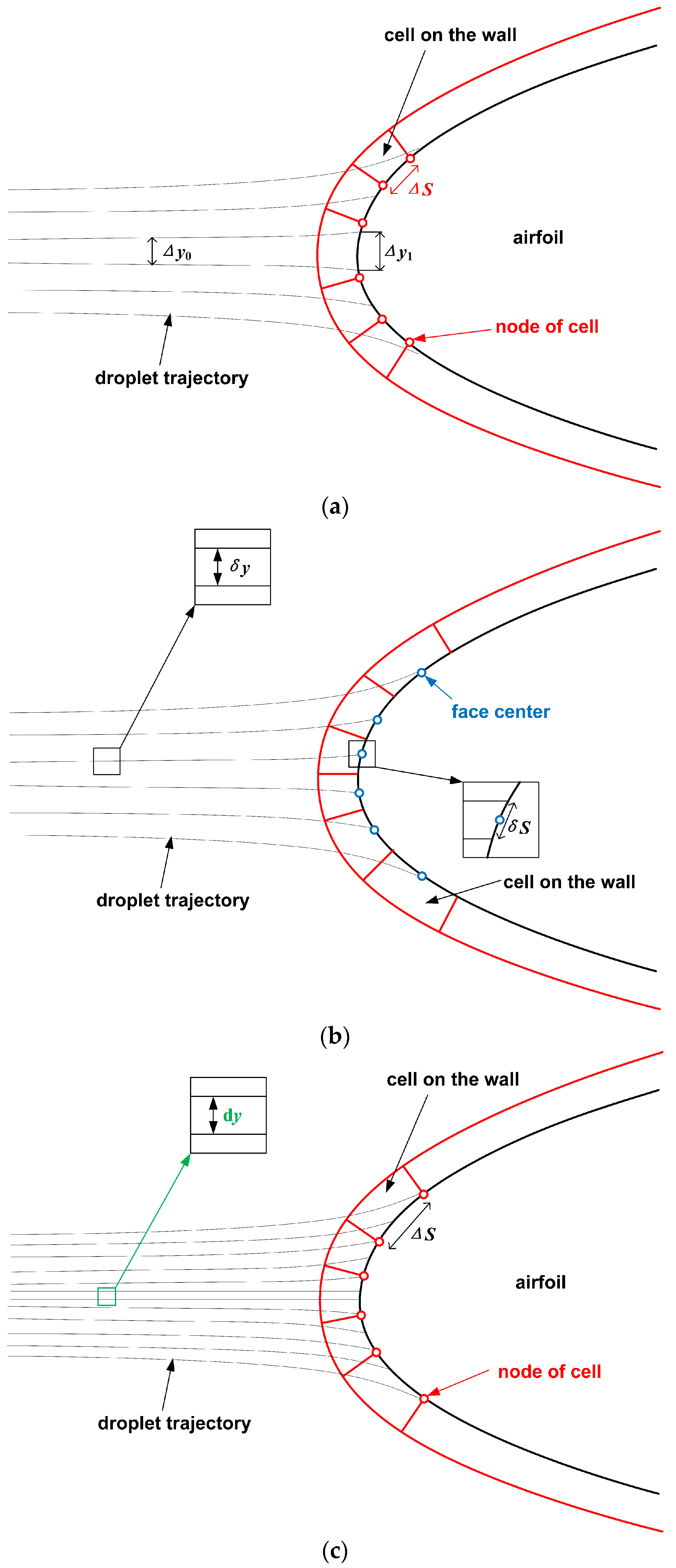
The Lagrangian method can track many droplets released from different locations, until they intersect with the wall surface or leave the computational domain. And the impingement amount and distribution characteristics of supercooled water droplets on the aircraft surface are obtained from the calculation on the collection efficiency. Three calculation methods, including the traditional flow tube method, the local flow tube method, and the statistical method, are established for the local collection efficiency, based on the different trajectories of the water droplets and the positional characteristics of the surface control volumes.
Firstly, a traditional flow tube method is developed, as shown in Figure 1a. For the tracked droplet trajectories that collide with the current surface control volume (the cell on the wall), the two trajectories closest to the two nodes of the cell are found on the wall. These two trajectories form a flow tube, and the local collection efficiency β can be defined by the width of the tube at the far field Δy0 and the distance between the impingement points of the two trajectories Δy1 [13]:
β = y 0 y 1
It is obvious that the traditional flow tube method represents the droplet impingement characteristics within a relatively large distance of the surface control volume. Similarly, the collection efficiency of the current control volume can also be represented by any two droplet trajectories that terminate on the surface. Therefore, we also select two very close trajectories, above and below the face center of the cell on the wall, to calculate the local collection efficiency, as shown in Figure 1b. Due to the fact that the trajectories of water droplets are calculated independently, the distance between the two trajectories at the free field δy can be even smaller than 10 μm, the order of the diameter of supercooled water droplets [24]. Then, the collection efficiency can be obtained using the local flow tube method [6]:
β = δ y δ S
where δS is the surface distance of the local flow tube. It can be seen that the collection efficiency at the center of the cell on the wall is used to represent the droplet impingement characteristics of the current control volume, using the local flow tube method.
On the other hand, considering the effects of water droplet trajectory intersection on the flow tube, a statistical method is established to obtain the local collection efficiency, as shown in Figure 1c. If the distance between adjacent droplets in the far field is dy, and the number of droplet trajectories ending at the current control volume is N, the local collection efficiency β can be defined as follows [7]:
β = N · d y S
where ΔS is the surface length of the cell on the wall. The droplet collection efficiency, based on the statistical method, represents the overall droplet impingement characteristics of the control volume.
In terms of implementation in the present work, the upper and lower limits corresponding to the impingement points are first determined by releasing a few particles, from a large distance, in front of the aircraft surface. Afterwards, a large number of supercooled water droplets are released inside the limits, and the number N of droplet trajectories intersecting the wall surface for each control volume is recorded. At the same time, the distance between the droplet impingement point and the node of the surface cell is calculated to find the nearest trajectory to the node for the traditional flow tube method, while the trajectories used in the local flow tube method are obtained by comparing the impact location and the face center of the cell. Finally, according to Equations (7)–(9), the local collection efficiencies are calculated using the traditional flow tube method, local flow tube method, and statistical method, respectively. As the number of released droplets increases, the impingement distance of Δy1 gradually tends toward the surface length of ΔS. The impact points used in the traditional flow tube method are getting closer and closer to the nodes of the surface cell, gradually representing the overall impingement characteristics of the control volume. Meanwhile, the value of δy in Equation (8), for the local flow tube method, becomes smaller with a shorter distance from the cell center, and the results increasingly express the collection efficiency at the midpoint of the surface control volume. In addition, when more and more droplets impact each surface control volume, the particle number independence can be obtained for the statistical method.

3. Results and Analysis

3.1. Method Validation

To verify the three methods for the collection efficiency in the Lagrangian framework, an NACA 0012 airfoil with a chord length of 1 m as in Ref. [29] is selected, as shown in Figure 2. The calculation conditions are as follows: the flight Mach number is 0.4, the angle of attack is 5°, the ambient temperature is 300 K with the corresponding pressure of 1 atm, and the supercooled water droplet has a single particle size with a diameter of 16 μm.
Figure 2 also shows the trajectories of the water droplets tracked by the Lagrangian method in the air flow field and the control volumes around the NACA 0012 airfoil. When approaching the wall, the air stagnates at the stagnation point on the lower surface and drastic changes in the velocity appear around the airfoil. The water droplets deflect toward both sides of the airfoil from the stagnation point. Some trajectories terminate on the airfoil surface, as shown in Figure 2, and the impingement points are recorded in the corresponding control volume. The bypass water droplets continue to deflect and form a shaded region due to the obstruction of the airfoil. In addition, the water droplets far away from the airfoil deviate less from the streamline, and the ones close to the wall are likely to deviate much more sharply due to greater resistance. Thus, it is easy to form a region near the airfoil where the droplet trajectories gather, known as the enhanced region of water droplet concentration. For a positive angle of attack, the density of the trajectories above the upper surface of the airfoil is higher and overlapping and crossing phenomena will occur.
After increasing the number of water droplets released, the average number of water droplets hitting a certain surface control volume reaches several hundred to achieve number independence. Then, the relative distance characteristics of the impact locations and the cell points of the surface control volume are analyzed. And the droplet collection efficiency can be obtained based on the established calculation methods. It can be seen from Figure 3 that the distributions of the local water collection efficiency for the three calculation methods are consistent. All the curves reach the maximum value at the stagnation point near the lower surface. Along the upper and lower surface of the airfoil, the collection efficiency gradually decreases to zero at the impingement limits. The collection efficiency of the three methods are in good agreement with that in Ref. [29], verifying the effectiveness and accuracy of the established methods. From the enlarged part of the figure, all the curves fluctuate around the stagnation point, similarly with the Lagrangian result in Ref. [29]. The fluctuation related to the local flow tube method is slightly more severe than those of the other two methods. One possible reason could be that the droplet trajectories slightly deflect from the airstream lines around the stagnation point, and the calculation accuracy to track the particle trajectories and impact points needs to be very high, especially for the local flow tube method.

3.2. Comparison for an S-Shaped Duct

According to a previous study [7], the motion of water droplets is deflected by upstream bodies and, then, the droplets hit downstream surfaces. The impingement characteristics of the Eulerian method and the Lagrangian method are no longer consistent. Considering the situation, the results of the collection efficiency in the Lagrangian framework are compared among the three different methods. An S-shaped duct with a long internal flow channel is selected for the 2D simulation, where the droplet motion will be greatly deflected. A semicylinder is set at the rear of the duct to represent an engine cone, and the geometric model of the whole S-shaped duct can be seen in Figure 4. The simulation conditions are as follows: the freestream velocity is 0.2 in relation to the Mach number with a 0° angle of attack, the ambient temperature is 263.15 K, and all the outlet pressures, including the outside engine wall and the engine duct exit are set to 1 atm. An ideal gas and droplet diameter of 50 μm is chosen.
Figure 4 shows the air flow field and the streamlines of the S-shaped duct. The air enters the S-shaped duct and changes its direction along the internal duct wall. Then, it hits the stagnation point on the leading edge of the cone, located on the upper cone surface. Finally, the air flows downstream around the semicylinder surface and leaves the computational domain. Based on the obtained air flow field, the water droplet trajectories inside the S-shaped duct and the impact locations on the cone surface are calculated in the Lagrangian framework, as shown in Figure 5. When the water droplets move into the S-shaped duct with the air flow, the deflection of the air flow drives the deflection of the water droplets due to the wall diversion effect. As the water droplets move downstream of the duct, the density of the droplet trajectories in front of the semicylinder varies in the y direction. The lower position has a larger trajectory density and a smaller distance between the trajectories. Figure 5 also shows that the trajectories of the water droplets deflected along the duct wall have no obvious overlap or crossing.
The local collection efficiency on the surface of the semicylinder in the S-shaped duct is compared for the three methods, as shown in Figure 6. In the figure, s is the surface distance along the cone surface. The leading edge of the semicylinder is at the location s = 0, and the value of s is positive on the upper surface. The leading edge of the semicylinder has a large water collection efficiency and the maximum amount is near the stagnation point on the upper surface. Then, the water collection efficiency gradually decreases along the upper and lower surfaces. The water droplets impact the entire upper surface, while the lower surface has a very small impingement range. The collection efficiency is in good agreement among the three calculation methods. The fluctuations are found around the stagnation point for all the three methods, and the curve for the local flow tube method fluctuates more severely, possibly due to the requirement for high calculation accuracy. Therefore, the three calculation methods in the Lagrangian framework are all effective and feasible to capture the water droplet collection efficiency when the motion of a water droplet is deflected without any overlap or crossing of the trajectories.

3.3. Comparison for a 2D Engine Cone Section with Outflow Film

In order to compare the calculation methods for collection efficiency under the effects of the overlap and crossing of droplet trajectories, a 2D engine cone section with a hot-air film-heating anti-icing system [11,30] is used as a test case for comparative analysis. The geometry can be seen in Figure 7. Water droplets may impact both on the frontal bump and the main cone surfaces. The water droplet motion and the collection efficiency of the main surface are affected not only by the air flow around the bump due to the shielding effect, but also by the blowing effect of the injection air from the internal part of the engine. The present work considers the mixing effect of the air flow inside and outside the cone section, but not the influence of the temperature change of the mixture. The simulation conditions are chosen as follows: the far-field velocity is 40 m/s, the water droplet diameter is 20 μm, and the inject air inlet is set as the velocity inlet boundary with a value of 4 m/s.
Figure 7 presents the air flow field and streamlines. The external freestream flows toward the object, stagnates at the leading edge of the frontal bump, and then flows backwards along its surface. Meanwhile, the internal air is accelerated in the channel inside the skin, enters the main air flow field to form an air film, and then flows downstream along the main cone surface. Figure 8 presents the trajectories of the water droplets around the object in the Lagrangian framework. The water droplets are deflected in front of the object, along with the air flow around the bump, and some of the water droplets impact the bump surface. The water droplets without impingement continue to move backwards and are deflected by the effects of the injection air, forming a water droplet shaded zone near the outlet of the internal air. The shaded zone produces a droplet enhancement region, with dense droplet trajectories. When the water droplets outside the shaded zone move downstream, some of them hit the main surface. Obviously, the droplet trajectories are greatly affected by the injection air. In addition, the trajectory deflection is more severe near the outlet of the internal air, while the change rate of the droplet direction is relatively small away from the wall surface. Therefore, there are obvious overlaps and crossings of the droplet trajectories in front of the main surface (Figure 8).
The traditional flow tube method, local flow tube method, and statistical method are compared to get the local collection efficiency of the main surface (Figure 9). Due to the shielding effects of the frontal bump and the influence of the internal air injection, there is no droplet impact on the leading edge and the front part of the main surface, as can be seen in Figure 8. And the local collection efficiency stays at 0 when x < 0.002 m, as shown in Figure 9. Backwards along the main surface, there is a region with a very large droplet collection efficiency, due to the influence of the water droplet enhancement effect outside the shaded zone. In this region, the overlaps and crossings of the droplet trajectories occur, as observed in Figure 8, and the liquid water content (LWC) is greater than that in far field, so the collection efficiency exceeds 1. The results of the three calculation methods are not the same under the influence of overlapping and crossing of the droplet trajectories. The value of the statistical method is relatively small, with slight fluctuation. The collection efficiency calculated by the traditional flow tube method fluctuates more compared with that of the statistical method. The local flow tube method fluctuates wildly, and the maximum value is more than 100. Downstream of the main surface, although the water droplet trajectories are still deflected under the influence of the bump and air blowing, there is no crossover of the trajectories (Figure 8). Therefore, the result curves in Figure 9 for the three calculation methods are relatively consistent, and they gradually decrease to 0 at the impingement limit, along the surface.

3.4. Comparison for an Icing Wind Tunnel

To analyze the influence of the overlap and crossover of droplet trajectories on the local collection efficiency using the three calculation methods in the Lagrangian framework, water droplet motion in a 2D icing wind tunnel [7] is simulated. As shown in Figure 10, the length of the calculation domain for the entire icing wind tunnel is 2 m. The height of the contraction section of the wind tunnel is 1 m, and the test section is 0.2 m high after the contraction section. The air and droplets flow from left to right. The inlet of the wind tunnel (x = 0 m) is set as the constant velocity, where the water droplets are evenly distributed, and the droplet speed is the same as the air of 50 m/s. The outlet of the wind tunnel is set to a constant pressure of 1 atm. The water droplet diameter is 60 μm. The water droplets leave the calculation domain when they reach the exit, which can be considered as impacting the outlet boundary. Therefore, although there is no water collection efficiency for the outlet boundary, the definitions of β in Equations (7)–(9) are used to study the distribution characteristics of the impact points in the Lagrangian methods.
The air flow field and streamlines in the icing wind tunnel are shown in Figure 10. The air enters the tunnel horizontally and is deflected in the contraction section of the wind tunnel. Then, the air flow converges into the test section with the increase in velocity, and the streamlines gradually become parallel to the x-axis, until they exit from the outlet. At the same time, the water droplet trajectories change direction, along with the deflection of the air flow in the contraction section, and the droplets have a y-direction component velocity (Figure 11). Due to the occlusion of the contraction section wall, there is a water droplet shaded zone near the downstream surface. Outside of the shaded zone, the droplet trajectories become very dense, with many crossings and overlaps. Then, the water droplets with trajectory crossings and overlaps move into the test section. The distance between the droplets is getting closer and closer, and the overlapping and crossing will occur again in the middle of the test section. The droplet trajectories then separate after the overlapping and crossings, and the distance between the droplets increases afterwards. The water droplets entering the upper half inlet of the wind tunnel all leave the test section from the lower half of the outlet, indicating that all the water droplet trajectories have crossed.
The β of the outlets, using the three methods, are shown in Figure 12. Due to the concentration of the water droplets in the test section, the β of the tunnel outlet should be greater than 1. Generally, the β has a maximum value at the center of the outlet, and gradually decreases along the upper and lower sides. Near the impingement limits, the β increases sharply as a result of the droplet enhancement region, with trajectory crossings and overlaps produced by the contraction section wall. The results from the three methods are in good agreement among most of the intervals, but differ greatly near the impingement limits. The local flow tube method gives the maximum water collection efficiency, but the others give much lower values. The result from the statistical method is the least among the three methods. The effects of the trajectory crossings and overlaps on the three methods are discussed in the next section.

4. Discussions

Based on the above results, the droplet impingement characteristics for trajectory overlaps and crossings are very complex. The following schematic diagram (Figure 13) is used for analysis and discussion of the trajectory crossings. Under the different trajectory intersection conditions, as shown in Figure 13, the numbers of the trajectories ending in the control volume are all recorded as obtaining the impingement water mass directly, and the collection results from the statistical method involve all the effects of the intermediate processes. Therefore, the statistical method could be relatively accurate under trajectory crossing and overlap conditions, and it represents the overall droplet impingement characteristics of the control volume, as described in Section 2.
For the traditional flow tube method, the flow tube in Figure 13a could be equivalently represented by the dashed lines, while the tube walls in Figure 13b,c would be the trajectories of No. 1 and No. 3. In the situations shown in Figure 13a,b, the large flow pipe would include all the water droplet trajectories that collide with the control volume, and the results would still be consistent with that of the statistical method. However, when the trajectories cross like the condition in Figure 13c, some trajectories pass through the flow tube walls, and the number of trajectories entering the flow tube is different from that of the exit. The water droplet mass at the inlet and outlet of the flow tube are no longer consistent, resulting in a different collection efficiency from that of the statistical method.
The tube walls in the local flow tube method are very close. When the distribution pattern of the trajectory crossings is consistent, the influence of the crossings is relatively average throughout the control volume, as shown in Figure 13a. The collection efficiency of the local flow tube method is the same as that of the other two methods, just like the results around the center of the icing wind tunnel outlet. However, in the situations shown in Figure 13b,c, the impact locations are unevenly distributed within the control volume. Therefore, the width of the local flow tubes differ very much at various positions, and the local collection efficiency at the center point of the control volume could be very different from that of the other two methods. By comparing Figure 13b,c, the local flow tube method is affected more by the trajectory crossings than the traditional flow tube method, since a larger flow tube can cover more regions of the trajectory crossings.
In practical situations, the distribution and effects of the trajectory crossings and overlaps are more complex than those shown in Figure 13, and the difference in the results of the three methods may be greater. If the statistical method is considered to be the right one for the impingement characteristics under the droplet trajectory crossing and overlap conditions, the flow tube method might obtain deviating results in some regions and the deviation of the local flow tube method is larger. But the non-crossing of water droplet trajectories is not a necessary condition for the flow tube method. In addition, it can be seen from Figure 13 that the results under the trajectory crossing conditions can also be affected by the surface mesh density, which will be considered in future research.

5. Conclusions

In the Lagrangian framework, a traditional flow tube method, a local flow tube method, and a statistical method to establish the water collection efficiency are established to study the impingement characteristics of supercooled water droplets under icing conditions. The droplet movement trajectories and collection efficiency for an NACA 0012 airfoil, an S-shaped duct, a 2D engine cone section with injection air film, and an icing wind tunnel are simulated and compared, and the main conclusions are as follows. If the water droplet trajectory is not affected by the upstream effects, the collection efficiencies obtained by the three calculation methods are consistent. The results for the NACA 0012 airfoil are in good agreement with the data in the literature, and the accuracy and effectiveness of the three methods in regard to the water collection efficiency are verified in the Lagrangian framework. When the water droplet trajectories are deflected by the upstream surface or the injection air without any trajectory overlap or crossing, the collection efficiencies are applicable and consistent for the three calculation methods. But if there is overlapping and crossing of the trajectories before the water droplets impact the wall surface, the collection efficiencies from the three methods might be different. The statistical method is relatively accurate. However, a non-crossing droplet trajectory is not a necessary condition for the flow tube method. Generally, the statistical method is recommended for the calculation of droplet impingement characteristics under complex conditions in the Lagrangian framework. With limited computing resources, the flow tube method could be used for rapid evaluation, but the local flow tube method cannot achieve higher accuracy than the traditional method. Further analysis will be carried out for more complex surfaces and 3D cases with the effects of a surface mesh, and such experimental validation should be carried out under conditions with the overlap and crossing of the droplet trajectories.

Author Contributions

Conceptualization, X.S., C.X. and G.L.; methodology, X.S. and G.L.; software, Y.N.; validation, H.W.; formal analysis, H.W.; investigation, C.X.; resources, L.W.; data curation, X.S.; writing—original draft preparation, X.S., H.W. and G.L.; writing—review and editing, C.X., Y.N. and L.W.; visualization, H.W.; supervision, G.L.; project administration, X.S.; funding acquisition, Y.N. and L.W. All authors have read and agreed to the published version of the manuscript.

Funding

This research was funded by the National Natural Science Foundation of China (No. 51806008), the Open Fund of Key Laboratory of Rotor Aerodynamics (No. RAL202104-2), and Shenyang Key Laboratory of Aircraft Icing and Ice Protection.

Data Availability Statement

The data used to support the findings in this study are available from the corresponding author upon request.

Conflicts of Interest

No conflicts of interest exist.

References

  1. Cao, Y.; Tan, W.; Wu, Z. Aircraft icing: An ongoing threat to aviation safety. Aerosp. Sci. Technol. 2018, 75, 353–385. [Google Scholar] [CrossRef]
  2. Yamazaki, M.; Jemcov, A.; Sakaue, H. A Review on the Current Status of Icing Physics and Mitigation in Aviation. Aerospace 2021, 8, 188. [Google Scholar] [CrossRef]
  3. Zhao, H.; Zhu, C.; Zhao, N.; Zhu, C.; Wang, Z. Experimental Research on the Influence of Roughness on Water Film Flow. Aerospace 2021, 8, 225. [Google Scholar] [CrossRef]
  4. Lou, Y.; Bu, X.; Shen, X.; Lin, G.; Zhang, R.; Zeng, F.; Jin, H.; Ma, K.; Wen, D. Simulation of and Experimental Research on Rivulet Model on Airfoil Surface. Aerospace 2022, 9, 570. [Google Scholar] [CrossRef]
  5. Jiang, X.; Wang, Y. Studies on the Electro-Impulse De-Icing System of Aircraft. Aerospace 2019, 6, 67. [Google Scholar] [CrossRef]
  6. Habashi, W. Handbook of Numerical Simulation of In-Flight Icing; Springer: Cham, Switzerland, 2023. [Google Scholar] [CrossRef]
  7. Shen, X.; Zhao, W.; Qi, Z.; Lin, G.; Wang, L. Analysis of numerical methods for droplet impingement characteristics under aircraft icing conditions. Aerospace 2022, 9, 416. [Google Scholar] [CrossRef]
  8. Bourgault, Y.; Boutanios, Z.; Habashi, W.G. Three-dimensional Eulerian approach to droplet impingement simulation using FENSAP-ICE, part 1: Model, algorithm, and validation. J. Aircr. 2000, 37, 95–103. [Google Scholar] [CrossRef]
  9. Tong, X.; Luke, E. Eulerian simulations of icing collection efficiency using a singularity diffusion model. In Proceedings of the 43rd AIAA Aerospace Sciences Meeting and Exhibit, Reno, NV, USA, 10–13 January 2005. [Google Scholar]
  10. Norde, E.; Weide, E.; Hoeijmakers, H. Eulerian method for ice crystal icing. AIAA J. 2018, 1, 222–234. [Google Scholar] [CrossRef]
  11. Shen, X.; Tan, Y.; Yu, R.; Liu, X.; Lin, G.; Xu, Z.; Guo, Y. Effects of upstream component and air injection on water droplet impingement characteristics for downstream surfaces. Int. J. Aerosp. Eng. 2021, 2021, 2698028. [Google Scholar] [CrossRef]
  12. Iuliano, E.; Brandi, V.; Mingione, G. Water impingement prediction on multi-element airfoils by means of Eulerian and Lagrangian approach with viscous and inviscid air flow. In Proceedings of the 44th AIAA Aerospace Sciences Meeting and Exhibit, Reno, NV, USA, 9–12 January 2006. [Google Scholar]
  13. Wright, W. User Manual for the NASA Glenn Ice Accretion Code LEWICE Version 2.2.2; NASA-CR-2002-211793; NASA Glenn Research Center: Cleveland, OH, USA, August 2002. [Google Scholar]
  14. Pierzyna, M.; Burzynski, D.; Bansmer, S.; Semaan, R. Data-driven splashing threshold model for drop impact on dry smooth surfaces. Phys. Fluids 2021, 33, 123317. [Google Scholar] [CrossRef]
  15. Burzynski, D.; Bansmer, S. Droplet splashing on thin moving films at high Weber numbers. Int. J. Multiph. Flow 2018, 101, 202–211. [Google Scholar] [CrossRef]
  16. Burzynski, D.; Roisman, I.; Bansmer, S. On the splashing of high-speed drops impacting a dry surface. J. Fluid Mech. 2020, 892, A2. [Google Scholar] [CrossRef]
  17. Burzynski, D.; Bansmer, S. Role of surrounding gas in the outcome of droplet splashing. Phys. Rev. Fluids 2019, 4, 073601. [Google Scholar] [CrossRef]
  18. Wang, C.; Chang, S.; Leng, M.; Wu, H.; Yang, B. A two-dimensional splashing model for investigating impingement characteristics of supercooled large droplets. Int. J. Multiph. Flow 2016, 80, 131–149. [Google Scholar] [CrossRef]
  19. Cao, Y.; Xin, M. Numerical Simulation of SLD Icing Phenomenon: A Review. Arch. Comput. Methods Eng. 2020, 4, 1231–1265. [Google Scholar] [CrossRef]
  20. Baumert, A.; Bansmer, S.; Trontin, P.; Villedieu, P. Experimental and numerical investigations on aircraft icing at mixed phase conditions. Int. J. Heat Mass Transf. 2018, 123, 957–978. [Google Scholar] [CrossRef]
  21. Papadakis, M.; Rachman, A.; Wong, S.; Yeong, H.; Hung, K.; Vu, G.; Bidwell, C. Water Droplet Impingement on Simulated Glaze, Mixed, and Rime IceAccretions; NASA/TM-2007-213961; NASA Glenn Research Center: Cleveland, OH, USA, October 2007. [Google Scholar]
  22. Papadakis, M.; Wong, S.; Rachman, A.; Hung, K.; Vu, G.; Bidwell, C. Large and Small Droplet Impingement Data on Airfoils and Two Simulated Ice Shapes; NASA/TM-2007-213959; NASA Glenn Research Center: Cleveland, OH, USA, October 2007. [Google Scholar]
  23. Villedieu, P.; Trontin, P.; Chauvin, R. Glaciated and mixed phase ice accretion modeling using ONERA 2D icing suite. In Proceedings of the 6th AIAA Atmospheric and Space Environments Conference, Atlanta, GA, USA, 16–20 June 2014. [Google Scholar]
  24. Xie, L.; Li, P.; Chen, H.; Liu, H. Robust and efficient prediction of the collection efficiency in icing accretion simulation for 3D complex geometries using the Lagrangian approach I: An adaptive interpolation method based on the restricted radial basis functions. Int. J. Heat Mass Transf. 2020, 150, 119290. [Google Scholar] [CrossRef]
  25. Hamed, A.; Das, K.; Basu, D. Numerical simulations of ice droplet trajectories and collection efficiency on aero-engine rotating machinery. In Proceedings of the 43rd AIAA Aerospace Sciences Meeting and Exhibit, Reno, NV, USA, 10–13 January 2005. [Google Scholar]
  26. Breer, M.D.; Goodman, M.P. Three-Dimensional Water Droplet Trajectory Code Validation Using an ECS Inlet Geometry; NASA Contractor Report 191097; NASA Glenn Research Center: Cleveland, OH, USA, May 1993. [Google Scholar]
  27. Wang, S.; Loth, E. Droplet impact efficiency on aerodynamic surfaces with a globally Eulerian/locally Lagrangian method. J. Aircraft. 2016, 1, 104–113. [Google Scholar] [CrossRef]
  28. Ansys Inc. Ansys FLUENT User’s Guide, Software Package, Ver. 19.1; Ansys Inc.: Canonsburg, PA, USA, 2019. [Google Scholar]
  29. Wirogo, S.; Srirambhatla, S. An Eulerian Method to Calculate the Collection Efficiency on two and Three Dimensional Bodies. In Proceedings of the 41st Aerospace Sciences Meeting and Exhibit, Reno, NV, USA, 6–9 January 2003. [Google Scholar]
  30. Dong, W.; Zhu, J.; Zheng, M.; Chen, Y. Thermal analysis and testing of nonrotating cone with hot-air anti-icing system. J. Propuls. Power 2015, 31, 896–903. [Google Scholar] [CrossRef]
Figure 1. (a) Traditional flow tube method. (b) Local flow tube method. (c) Statistical method. Calculation methods for local collection efficiency in the Lagrangian framework.
Aerospace 11 00172 g001
Figure 2. Droplet trajectories in the airflow field and control volumes around an NACA 0012 airfoil.
Aerospace 11 00172 g002
Figure 3. Comparison of collection efficiencies, with the reference result [29] for the NACA 0012 airfoil.
Aerospace 11 00172 g003
Figure 4. Air flow field and streamlines of the S-shaped duct.
Aerospace 11 00172 g004
Figure 5. Droplet trajectories around the semicylinder in the S-shaped duct.
Aerospace 11 00172 g005
Figure 6. Comparison of the collection efficiencies obtained using the three methods for the S-shaped duct.
Aerospace 11 00172 g006
Figure 7. Air flow field and streamlines of the 2D engine cone section with outflow air film.
Aerospace 11 00172 g007
Figure 8. Droplet trajectories in the 2D engine cone section, with outflow air film.
Aerospace 11 00172 g008
Figure 9. Comparison of the collection efficiencies for the 2D engine cone section, with outflow air film, using the three methods.
Aerospace 11 00172 g009
Figure 10. Air flow field and streamlines of the icing wind tunnel.
Aerospace 11 00172 g010
Figure 11. Droplet trajectories in the icing wind tunnel.
Aerospace 11 00172 g011
Figure 12. Comparison of the β at the outlet for the icing wind tunnel using the three methods.
Aerospace 11 00172 g012
Figure 13. (a) Situation 1. (b) Situation 2. (c) Situation 3. Schematic diagram of the trajectory crossings in different situations.
Aerospace 11 00172 g013
Disclaimer/Publisher’s Note: The statements, opinions and data contained in all publications are solely those of the individual author(s) and contributor(s) and not of MDPI and/or the editor(s). MDPI and/or the editor(s) disclaim responsibility for any injury to people or property resulting from any ideas, methods, instructions or products referred to in the content.

