
The Modeling and Control of a Distributed-Vector-Propulsion UAV with Aero-Propulsion Coupling Effect

College of Aeronautics, Northwestern Polytechnical University, Xi’an 710072, China
*
Author to whom correspondence should be addressed.
Aerospace 2024, 11(4), 284; https://doi.org/10.3390/aerospace11040284
Submission received: 22 February 2024
/
Revised: 26 March 2024
/
Accepted: 3 April 2024
/
Published: 6 April 2024
(This article belongs to the Special Issue Aerodynamics, Flight Dynamics and Control of Advanced Air Mobility Vehicles)
Abstract
:A novel distributed-vector-propulsion UAV (DVPUAV) is introduced in this paper, which has the capability of Vertical takeoff and landing (VTOL), and can realize relatively high-speed cruise. As the core of the DVPUAV, the propulsion wing designed under the guidance of the integration idea is not only a lifting body but also a propulsion device and a control mechanism. However, this kind of aircraft has a series of difficult problems with complex aero-propulsion coupling, flight modes switching, and so many inputs and control coupling. In order to describe this coupling effect to improve the accuracy of dynamics, an aero-propulsion coupling model is developed, considering both computation reliability and real-time. Afterward, a unique control framework is designed for the DVPUAV. By optimizing control logic, this control framework realizes the decoupling of longitudinal and lateral directional control and even the decoupling of roll and yaw control. Next, based on the Iterative linear quadratic regulator (ILQR), a new Model Predictive Control (MPC) controller with the ability to solve complex nonlinear problems is proposed which achieves the unification of the controller for the full flight envelope. Finally, the good performance of the control framework and controller is verified in the whole process of the flight simulation from take-off to landing.
1. Introduction
In recent years, the low-carbon development model has been increasingly valued, and countries around the world have proposed the goal of carbon neutrality with rapid social development and the advancement of science and technology. In the aviation field, the concept of green aviation has gradually attracted more attention from research institutions and scholars [1,2]. Therefore, the distributed electric propulsion (DEP) system with more energy-efficient, eco-friendly and superior aerodynamic performance has become a research hotspot recently [3,4].
DEP consists of an array of propulsors distributed on the aircraft. Integrating propulsors into the fuselage or wing is the mainstream of DEP, which has great potential to realize the structural conformal design and the integration design of aerodynamic propulsion. Based on the boundary layer ingestion (BLI), the well-designed DEP has higher propulsive efficiency [5,6]. The aerodynamic performance of aircraft has also been improved due to the aero-propulsion coupling from DEP. The Europe program “Clean Sky 2” pointed out that the maximum lift coefficient could even reach 4.5 in the 2D scenario affected by ducted fans [7]. In addition, through wind tunnel tests and CFD computation [8], it is confirmed that DEP has the positive characteristics of increasing lift and reducing drag at low airspeed. DEP is considered a disruptive technology in the aviation industry [9,10] since it has enormous potential to improve aircraft aerodynamic efficiency, endurance, environmental friendliness and robustness.
Some researchers [11] not only hope to give full play to the aerodynamic advantage of DEP technology but also hope that the aircraft has the ability of thrust vector control (TVC) to expand the flight envelope and realize short takeoff and landing (STOL) and even vertical takeoff and landing (VTOL). VTOL aircraft have two attractive advantages: flexible take-off and landing without the requirement for airport conditions, and a long endurance with high-speed cruise ability. In terms of military use, it could be used for mountain battles and VTOL from ships, while more and more VTOL urban aircraft are gradually emerging for civil use. Therefore, based on its significant advantages and great application prospects, VTOL aircraft have attracted more attention in recent years [12,13]. By paying a certain price for structural weight, the DEP system could be tilted to meet the lift (thrust) requirement of aircraft in the event of aerodynamic failure. Now, there are a number of configurations proposed and developed for a new emerging “air-taxi” market in the civil area, such as the S2 aircraft of Joby Aviation and the Lilium Jet of Lilium Aviation.
Although DEP aircraft with TVC have technical advantages, they face complex dynamics and control problems. The problem of dynamics mainly comes from the aero-propulsion coupling of the DEP system and the large variation of dynamics characteristic in the flight envelope. As for flight control, there are difficulties with too many inputs caused by distributed actuators, the coupling of lateral directional control and so on. Therefore, it is an enormous challenge to solve the aerodynamics-propulsion-dynamics-control problem of DEP aircraft.
In order to track longitudinal velocity trajectory, Rohr et al. [14] formulated a high-level Nonlinear Model Predictive Control (NMPC) to optimize throttle, tilt-rate and pitch-angle setpoints for a small tiltwing hybrid unmanned aerial vehicle (UAV). Xia et al. [15] proposed a longitudinal MPC controller for a flying-wing UAV with tilt DEP, which realized a satisfactory control effect for the rotor mode, transition process and fixed-wing mode. Although some air vehicles do not adopt DEP technology, they have similar characteristics in dynamics and control to DEP aircraft with TVC. Liu et al. [16] attempted to apply a predictor-based adaptive roll and yaw controller for a rudderless quad-tiltrotor UAV and confirmed the feasibility of roll and yaw control decoupling via flight tests. Ahmed and Katupitiya [17] presented work about the design of a nonlinear control allocation algorithm and nonlinear feedforward compensations that could handle the increased nonlinearity inherent to a vectored-thrust quadcopter, and decoupling the translational and rotational motions. Bauersfeld et al. [18] proposed a unified control approach for tilt-rotor VTOL aircraft based on nonlinear MPC, which is verified in all flight modes through simulation and outdoor experiments. This method seems to be good enough, except that the computation burden of nonlinear MPC is too large. Mike and Guillaume [19] declared that the unified NMPC control approach outperforms the scheduled PID methodology [20,21] in all flight phases for a propeller-tilting hybrid UAV because the dynamic model is included in the MPC controller to optimize the control sequence.
As an advanced control method, MPC could predict the future behavior of the system by using the system model to solve optimization problems, thus obtaining control solutions [22]. However, for a long time, there has been a great challenge for MPC controllers about the high computational cost. Iterative linear quadratic regulator (ILQR) is an efficient algorithm featuring a super-linear convergence rate with linear complexity to deal with nonlinear optimal control problems [23]. This algorithm linearizes the dynamics by Taylor expansion; then, based on Bellman’s principle [24], the input sequence is obtained in the backward pass, while the state sequence is updated in the forward pass, finally, the optimal solution is obtained through cyclic iteration [25]. In recent years, the MPC based on ILQR methods has been gradually applied and achieved good results [15,26,27].
This paper introduces a distributed-vector-propulsion UAV (DVPUAV) as the research object, mainly focusing on the development of an aero-propulsion coupling model and the design of a control scheme. The main contributions of this paper lie in the proposed:
- An aero-propulsion coupling model (APCM) is developed to meet the requirements of flight dynamics and flight control. The proposed APCM is an analytical model and could balance computational accuracy and speed so that it has the capability to be directly applied to flight dynamics and control, which is the first attempt to the best of our knowledge.
- A unique control framework is designed for the DVPUAV, a system with complex control coupling and so many inputs. Based on the logic of baseline inputs plus longitudinal differential inputs or lateral directional increment inputs, the decoupling of longitudinal and lateral directional control as well as the decoupling of roll and yaw control are realized. The number of inputs is greatly reduced from 32 to 8, which is beneficial to reducing the computational burden.
- An MPC controller is presented based on ILQR, which is capable of efficiently solving nonlinear control problems with linear complexity. Therefore, this controller is suitable for the DVPUAV with an aero-propulsion coupling effect, which is a novel application in the field of VTOL aircraft. Moreover, this controller is a unified one for the full flight envelope, which is fundamentally superior to the conventional VTOL controller.
The remainder of this manuscript is organized as follows. The features and advantages of the DVPUAV are presented in Section 2. Then, the dynamics model of the DVPUAV is developed, where emphasis is placed on the modeling of the aero-propulsion coupling effect of the propulsion wing. Section 3 introduces the flight strategy, control framework and controller in detail. Afterwards, the model verification and simulation analysis are shown in Section 4. Lastly, Section 5 concludes the full manuscript.
2. Modeling of the DVPUAV
2.1. DVPUAV Conceptual Design
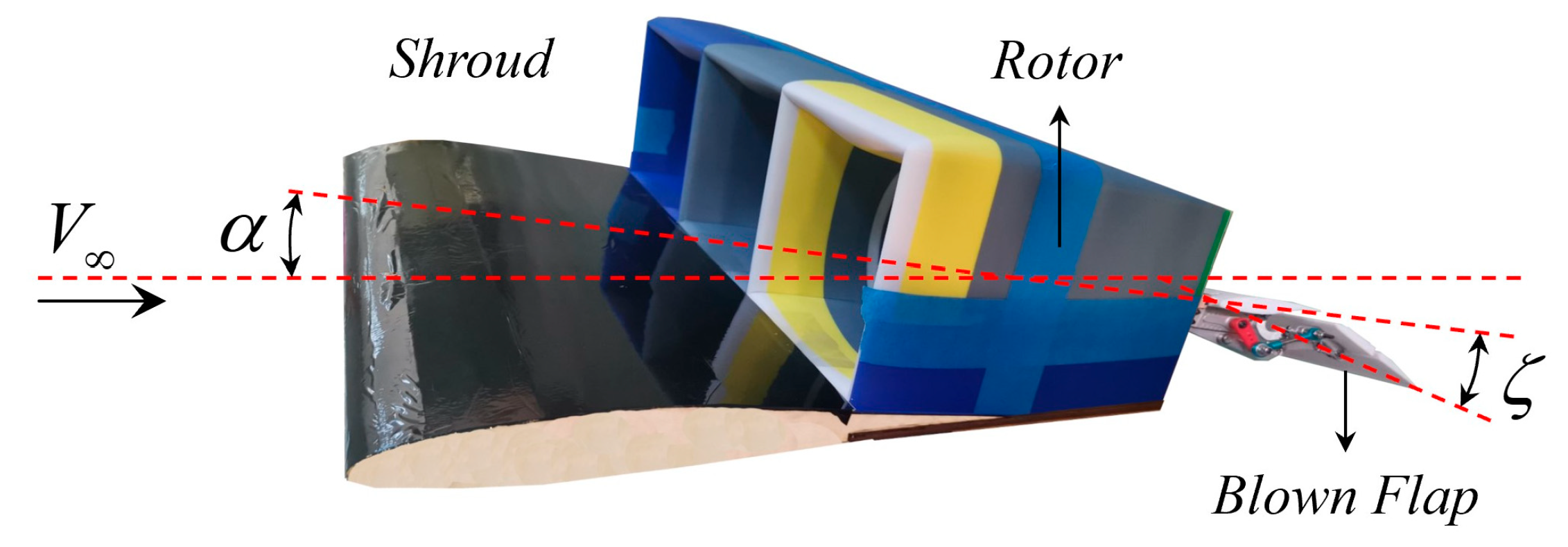
The DVPUAV adopts a tandem layout, consisting of a fuselage, front and rear propulsion wings (DVP system) and winglets as Figure 1 shows. The propulsion wing (please see Figure 2) is the core of the DVPUAV, including the shroud, the rotor inside the shroud, and the blown flap that could be deflected to change the thrust vector direction. Winglets have the function of adjusting the lateral stability on the one hand and suppressing the wingtip vortex to improve the UAV aerodynamic efficiency on the other hand.
The DVPUAV has two flight modes: slow mode and fast mode, the switch between them is realized through thrust vector control and attitude adjustment. In slow mode, the gravity of the UAV is mainly overcome by the thrust of the rotor and its coupled forces, around a deflection angle of the blown flap. While in fast mode, the aerodynamic forces play a role in overcoming gravity, with around a deflection angle of the blown flap. Please see Section 3.1 for more details.
The DVPUAV has two outstanding advantages: 1. Under the guidance of integrated design ideas, the propulsion wing is not only a lifting body but also a propulsion device and control mechanism, which realizes structure conformal design to optimize the structural form and reduce weight. 2. The aero-propulsion coupling effect brings beneficial effects on lift and thrust, and the control potential of the blown flap is significantly enhanced because of the jet-flow coupling.
2.2. Aero-Propulsion Coupling Model of Propulsion Wing
Existing research has clearly declared that there is a strong coupling effect between the aerodynamics and propulsion of the DEP system. The traditional analysis method based on engineering experience cannot describe the aero-propulsion coupling effect [28], and the numerical computation method represented by CFD cannot meet the real-time requirements of flight dynamics and control systems [29]. At present, there is still a lack of an aero-propulsion coupling model with reliable accuracy, fast computation speed and interpretability, and this model is the basis for solving the aerodynamics-propulsion-dynamics-control problem of DEP aircraft.
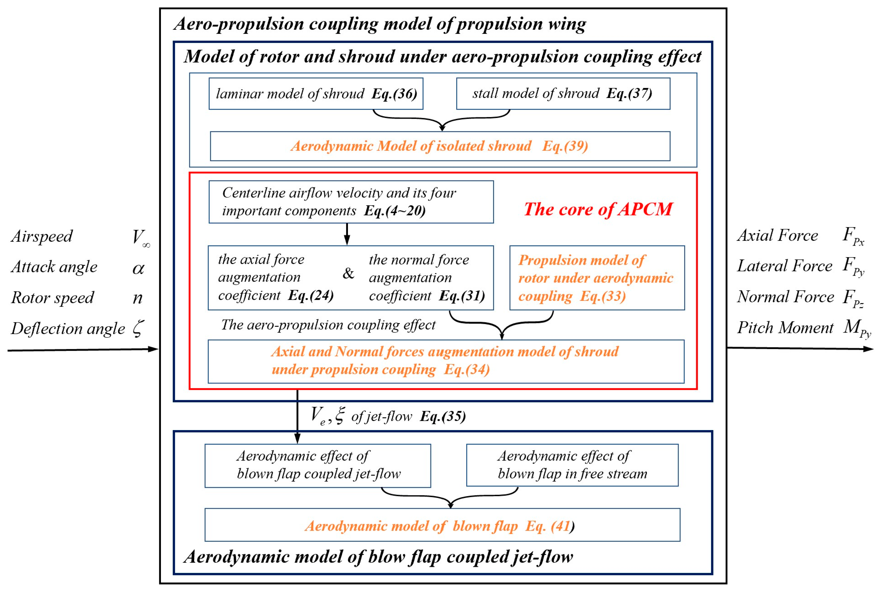
It should be noted that our aero-propulsion coupling model does not overly focus on accuracy, but rather on computation speed to provide real-time data for flight dynamics and control. The aero-propulsion coupling model is composed of a model of rotor and shroud under the aero-propulsion coupling effect and an aerodynamic model of blown flap coupled jet-flow, whose computation logic is shown in Figure 3.
2.2.1. Model of Rotor and Shroud under Aero-Propulsion Coupling Effect
The main parameters related to the shroud and rotor are shown in Figure 4. denote velocities of free-stream, exit flow and far-field flow, respectively, are the attack angle of the propulsion wing and the downwash angle of the exit flow, respectively, represent the equivalent angle of the upper and lower lips of the shroud, respectively, represents the axial distance from the ¼ chord length position of the lower lip to rotor disc, represents the axial distance from exit station to rotor disc, denote the radiuses of the lower lip, upper lip, rotor, rotor station (camber line) and exit station, respectively. Taking as a benchmark, length parameters are nondimensionalized as , respectively, where . Moreover, the most important stations are the rotor station and exit station, which will be mentioned multiple times in subsequent derivation.
The disk model [30] of the rotor could describe the flow changes through the rotor from upstream to downstream inviscid regions, so the rotor thrust could be written as
where , respectively, represent the pressure before as well as after the rotor disc.
The total thrust of the propulsion wing is composed of the rotor thrust and the shroud thrust caused by the induced low-pressure area of the shroud lip. Based on the momentum equation in integral form [31], from the upstream zone to the downstream outlet, the total thrust of the rotor and shroud is expressed as
where is the air density, representing the axial component of airspeed, axial velocities of rotor station and far-field, respectively.
Define the axial force augmentation coefficient of the shroud and the system thrust augmentation coefficient . Next, combining Equations (1) and (2), and Bernoulli’s equation, there is a key expression shown as following
Then, the airflow velocity on the centerline is derived from four important components: induced velocities by free-stream, by rotor disc, by airfoil camber of shroud, and by cross-sectional area variation (please see Figure 5). However, different from Werle [32,33], the induced effect by the airfoil camber of the shroud is divided into two parts for consideration, so that we can consider the conditions of asymmetric shroud lips or non-zero attack angle, and further analyze the changes in normal flow velocity on the centerline.
Taking as a benchmark [33,34], the dimensionless expression of axial velocity on the centerline in the internal passage is
where denotes dimensionless axial induced velocity by rotor disc, denotes the dimensionless axial induced velocities by airfoil camber of shroud, denotes the dimensionless axial induced velocity by area.
Similarly, the normal velocity could also be dimensionless based on ,
Furthermore, considering that on the centerline, and because of the center symmetry of the internal passage; the dimensionless normal velocity on the centerline in the internal passage is given by
where is dimensionless normal induced velocity by free-stream, is dimensionless normal induced velocity by airfoil camber of shroud.
The rotor disc and airfoil camber of the shroud are represented based on different vortex models, and then each induced velocity is gained based on the Biot–Savart Law. The rotor disk is modeled according to a semi-infinite cylindrical vortex [34],
where denotes the circulation term related to the rotor disc. There is at infinity downstream, and Equation (4) at . Then, it is easy to obtain as
The cross-sectional area of the rotor station is and that of the exit station is . When only considering the induced velocity by cross-sectional area variation, based on the law of mass conservation, there are expressions such as
where , represent the axial positions of the rotor station and exit station, respectively.
Referring to the vortex lattice method, the vortexes of the shroud are divided into two parts: 1. A straight line vortex is arranged in the 1/4 chord of the “epitaxial part” of the lower lip. 2. A circular vortex is arranged in the camber line of the shroud at the rotor station [23,34]. Define and as circulation term related to vortexes of the shroud, so the corresponding axial induced velocities are represented as
Similarly, the normal velocity on the centerline induced by a straight-line vortex could be expressed as
Next, the specific expressions of and are derived as follows.
Let Equation (4) be established at the rotor station,
By simple transformation, Equation (13) is updated as
where .
The flow rate in the shroud inlet increases under propulsion coupling, resulting in airflow contraction. To describe this phenomenon, we define the equivalent angle of airflow from the surrounding inlet to the center of the rotor disc as
So, the equivalent angles of upper and lower lips are and .
In addition, there is a mutual repulsion of the airflow during the contraction process, and it is considered that the repulsion velocity vector is symmetrical about the centerline. Therefore, when the inlet airflow approaches the rotor disk, the normal velocity of the typical airflow element could be approximately described as
According to the law of conservation of mass, . When the thrust of the rotor is zero, the exit state is close to the free-stream state, that is , so .
Then, based on Equation (5), the dimensionless normal velocities of the upper and lower symmetrical positions with radius to the centerline at the rotor station are, respectively, expressed as
Next, integrate (a) and (b) of Equation (17) into a new equation, and substitute Equation (16) into it,
where , , .
Therefore, the expression for circulation terms can be gained by combining Equations (14) and (18) as follows
Based on Equation (4), the axial velocity of the centerline at the exit station is written as,
where , , .
Assuming that the shroud is well designed, the static pressure at the exit station is basically restored to that of the free stream. Hence, based on the Bernoulli equation, there is . By substituting Equations (19) and (20) into Equation (21), the dimensionless axial velocity of the centerline at the rotor station could be expressed as
where , , .
Combining Equations (3) and (22), we obtain the specific expression for the system thrust augmentation coefficient
Naturally, the axial force augmentation coefficient of the shroud is written as
Based on Equation (6), the dimensionless normal velocity of the centerline at the exit station is given by
where .
Then, substituting Equation (19) into Equation (25) as
According to the law of conservation of mass, there is ,
where .
Referring to the engine nacelle [35], the normal force caused by aero-propulsion coupling is expressed as
where , .
Afterward, combining Equations (2) and (28) into a new equation written as
Bring Equation (27) into Equation (29), the relationship between the normal force increment of the shroud and the total thrust is written as follows
Therefore, the normal force augmentation coefficient of the shroud is obtained as
In fact, compared with an isolated rotor, the main influence of aerodynamic coupling on the rotor inside the shroud is to accelerate the axial flow velocity at the rotor station, resulting in a decrease in the attack angle of the rotor blade elements, thus leading to changes in the propulsion characteristics of the rotor. Therefore, based on momentum theory and blade element theory, we can gain the rough propulsion performance of the rotor inside the shroud. Then, by combining CFD numerical technology or wind tunnel experiment for parameter calibration, a reliable rotor propulsion model could be obtained like Equation (32),
Therefore, combining Equations (23), (24), (31) and (32), the axial and normal forces augmentation effect could be described as follows
Besides, with the combing momentum law and Bernoulli equation, the approximate value of can be obtained, then incorporating Equation (27), is expressed as
Furthermore, the velocity and downwash angle of exit flow (that is, the jet-flow for the blown flap) are written as
Aerodynamic model of the isolated shroud
As a wing segment with a special shape, the isolated shroud (without rotor) could be modeled with reference to lifting surface theory. Then, considering that the DVPUAV may face a high attack angle state during the takeoff and landing processes, stall correction should be added to improve the model.
The laminar model of the isolated shroud is given by
where are the lift coefficient at zero attack angle and lift curve slope, respectively, and are the zero-lift drag coefficient and the induced drag factor, respectively.
Next, referring to [36], the stall model of the isolated shroud is written as
where are terms related to maximum lift and drag coefficients, respectively.
Therefore, combining Equations (36) and (37), the aerodynamic coefficients of the isolated shroud are expressed as
where is slew factor with slew attack angle and slew rate .
Naturally, the aerodynamic model of the isolated shroud is given by
where is the reference area of the shroud, are the spin of the propulsion wing unit and the chord length of the shroud, respectively, is the lateral force coefficient of the isolated shroud, and is the sideslip angle.
2.2.2. Aerodynamic Model of Blown Flap Coupled Jet-Flow
The blown flap is affected by both free stream and jet-flow, its aerodynamic performance changes greatly because of jet-flow. Therefore, the aerodynamic forces of a blown flap could be divided into two parts to analyze. The first part is the original aerodynamic forces, and the second part is produced by the jet effect.
There is a relationship between the deflection angle of the wake and that of the blown flap . On the basis of the geometric relationship, the reaction force generated by jet deflection caused by the blown flap is , which could be decomposed into , in the jet-flow coordinate system [34]. In addition, the extra drag of the blown flap would occur due to the jet-flow.
Define as the blowing momentum coefficient and the relationship , where is the reference area of the shroud, and is the chord length of the blown flap. Then, the lift and drag coefficients are given by
where represent the aerodynamic derivatives of the blown flap related to the free stream, respectively, and represents the induced drag factor of the blown flap.
Therefore, the lift and drag of the blown flap could be gained,
Besides, the lateral force of the blown flap is ignored because it is a horizontal aerodynamic surface.
2.2.3. Forces and Moments of Propulsion Wing
denotes the propulsion wing coordinate system with the origin at the reference center of the propulsion wing (also the center of the rotor disc). Based on the models developed in Section 2.2.1 and Section 2.2.2, the forces of the propulsion wing are shown in Figure 6.
Taking the forces on the shroud and blown flap, transform to ,
Furthermore, we could obtain the generalized external forces of the propulsion wing unit as follows,
where , denote the distances between action positions of to the , respectively.
2.3. Nonlinear Dynamics Model
The definitions of coordinate systems and rotation transformation matrices are as follows,
: Coordinate system of the front propulsion wing.
: Coordinate system of the rear propulsion wing.
: Body coordinate system locates at c.g. with parallel axes to .
: Inertial coordinate system using North-East-Down coordinate.
Two important rotation transformation matrices from and to , respectively, are given by
where denotes the relative angle between the front propulsion wing and the rear propulsion wing.
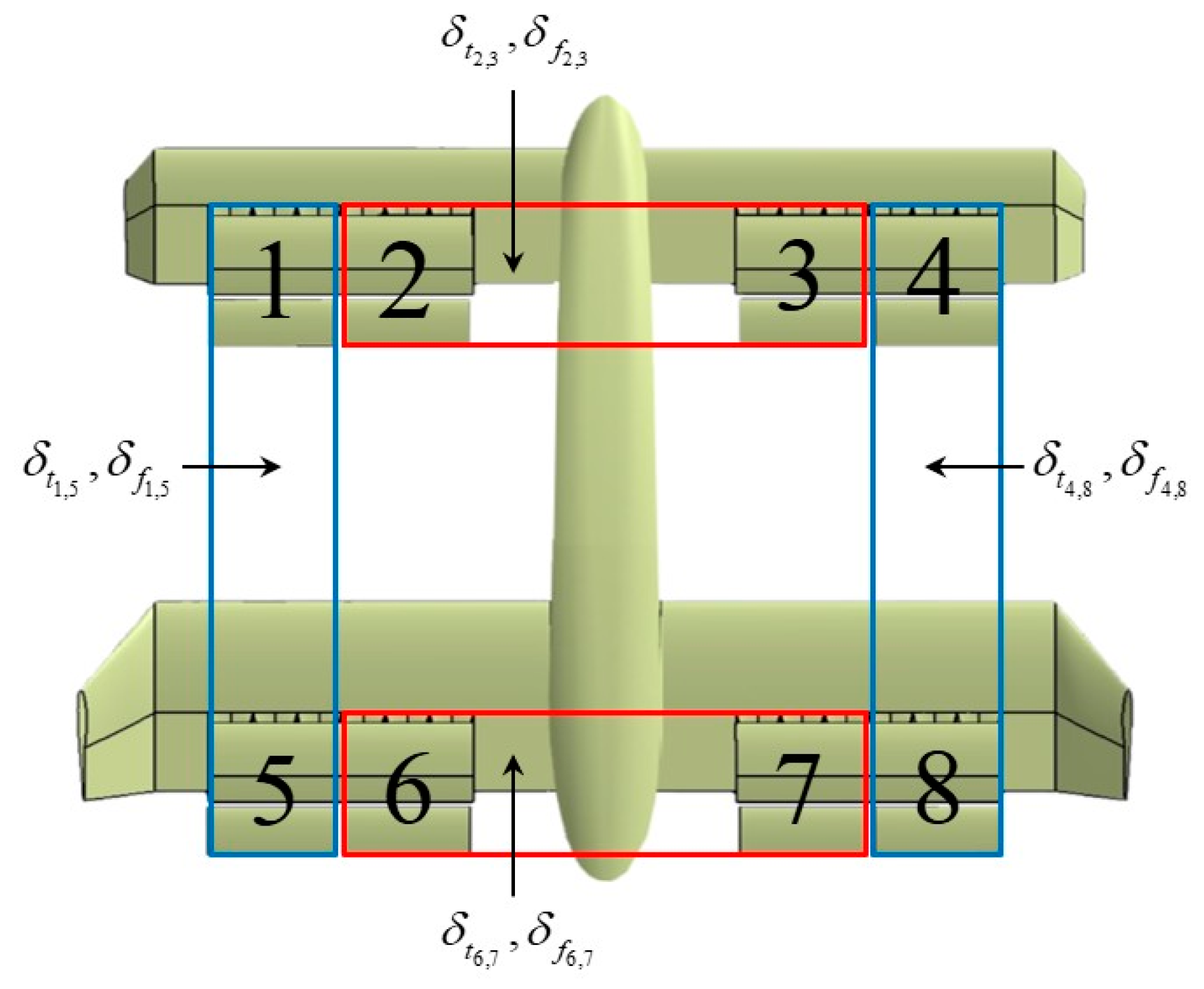
Each propulsion wing group is formed by three adjacent propulsion wing units. Due to the distributed layout of the DVPUAV, each propulsion wing group has different inputs () even airflow conditions (). There are eight sets of propulsion wing groups distributed on the front and rear wings, numbered and in sequence. Then, the forces of all propulsion wing groups would be transformed to the body coordinate system, in which the forces of the front wing are expressed as , and that of the rear wing are expressed as . Additionally, the relevant longitudinal, lateral and vertical distance parameters are defined as , and , respectively, as shown in Figure 7.
The external forces acting on the DVPUAV include gravity, aerodynamic/propulsion forces of front and rear propulsion wings and aerodynamic force of winglet and fuselage. All forces and moments are expressed in a body coordinate frame as follows
where represent the aerodynamic forces as well as the aerodynamic moments of the fuselage and winglets, respectively, and represents the gravity of the DVPUAV.
Furthermore, the nonlinear dynamic model, including the translation model and rotation model, could be formulated as follows
where represent the mass and moment of inertia of the DVPUAV, respectively, represents angular velocity vector, and represents velocity vector. Besides, because of the opposite rotation directions of the rotors of the adjacent propulsion wing units and the symmetrical distribution of the DVPUAV along the axis, the torque and gyroscopic moment of the propulsion wing are considered to cancel out within the system.
3. Control Scheme Design
3.1. Flight Strategy
A DVPUAV spanning a hovering state to a relatively high-speed state has a wider flight envelope than conventional UAVs. According to its characteristics, the flight modes of the DVPUAV can be divided into two categories (as shown in Figure 8): 1. The slow mode represented by the ultra-low-speed state, relies on the thrust and the aerodynamic force induced by the thrust to overcome gravity and has the ability of accurate position tracking. 2. The fast mode represented by cruise state is mainly based on aerodynamic lift to overcome gravity and has strong endurance. Unlike the rotor-fixed-wing hybrid aircraft, the two modes of the DVPUAV have a unified control logic, so there is no clear boundary between them. However, “transition flight” is still used to refer to the transition process between the two modes for better understanding.
In the slow mode, the DVPUAV puts down a blown flap to provide a larger normal force so as to fly at low airspeed or even at a fixed point. The fast mode is the main mode of task execution, which is almost the same as conventional UAV. The DVPUAV is unique in takeoff and landing processes, and has two patterns of takeoff and landing: VTOL and STOL. The DVPUAV making a vertical takeoff from the takeoff platform relies on the downward vector thrust to overcome gravity. Vertical landing could be achieved by landing the rear wheels first without using the takeoff platform. More aerodynamic lift is obtained through taxiing in STOL, but the required runway length is far less than that of conventional fixed-wing aircraft.
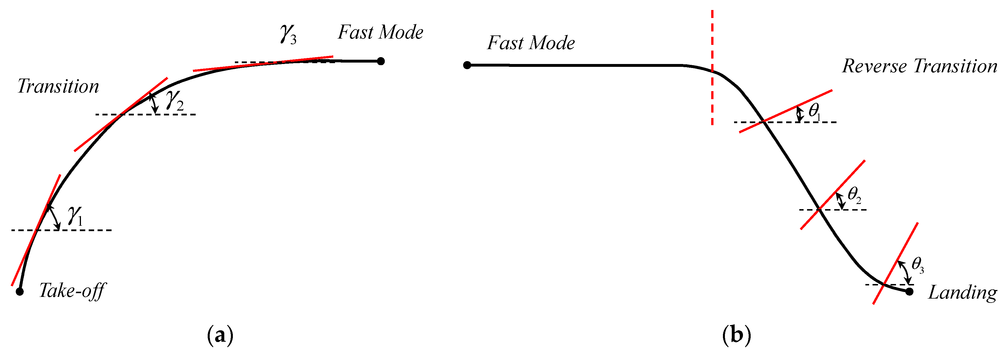
In this paper, VTOL is adopted. The takeoff process of the DVPUAV is referenced from the tailsitter UAV [37] as Figure 9 shows. The path angle changes from a large angle in the takeoff state to a small angle in the cruise state, which is beneficial to keep the attack angle in an ideal range. During the landing process, the aerodynamic drag is utilized for the DVPUAV deceleration [38] first and then the UAV lands in slow mode with the pitch angle gradually rising. The design of the takeoff and landing process is not the focus of this paper, so it is introduced briefly without too much detail.
3.2. Control Framework
Because of the complex configuration and special flight modes of the DVPUAV, there are many difficulties in flight dynamics and control leading to great challenges to flight. Specifically, predominant problems in flight control include too many inputs caused by distributed actuators, manipulation effectiveness differences of actuators between the two flight modes, and the problem of control coupling. Therefore, it is the primary step to clarify the control logic to establish the control framework.
- First Step: Inputs Grouping
The DVPUAV has many adjustable variables including 24 throttle inputs and eight deflection inputs as shown in Figure 10, leading to so many possible control combinations.
Hence, in order to achieve highly accurate flight control, a unique control framework is proposed in this paper. Each group propulsion wing consists of three adjacent propulsion wing units which are given the same control channel, so the number of inputs is reduced from 32 to 16. These inputs are sorted as and from left to right and from front to back, in which subscripts “” represent throttle input and deflection input, respectively.
- Second Step: Decoupling 1 (Longitudinal and Lateral Directional Control Decoupling)
The traditional flap has great longitudinal auxiliary control capability, while the outside propulsion wing groups are more efficient for roll and yaw control capability. Hence, as well as are arranged for longitudinal control, and as well as are arranged for lateral directional control, which could realize the decoupling of longitudinal and lateral directional control. (Please see Figure 11).
Next, the differential between front and rear vector thrust (including the magnitude and direction) realizes UAV pitch control, the vertical differential between left and right vector thrust realizes roll control, and the horizontal differential between left and right vector thrust realizes yaw control. Based on these control rules, the efficient flight control of the DVPUAV could be realized. Therefore, “2&3”, “6&7”, “1&5” and “4&8” are assigned to the same control channels, respectively, thus reducing the number of control inputs further to 8.
- Third Step: Decoupling 2 (Roll and Yaw Control Decoupling)
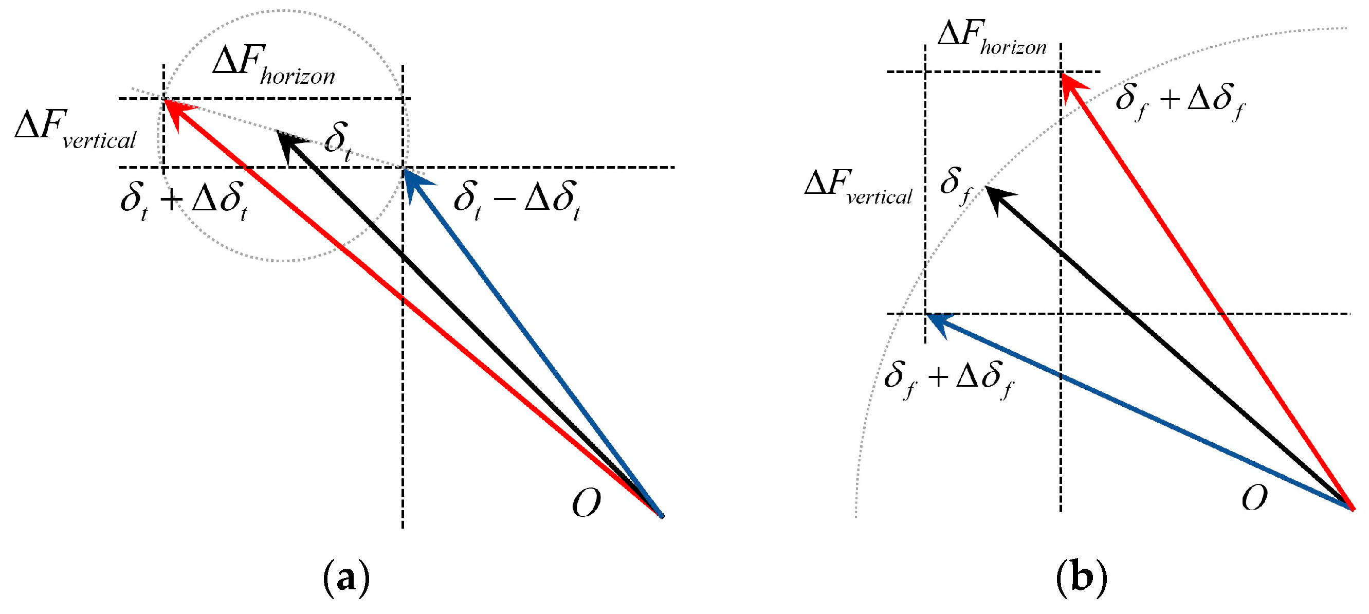
Due to the aero-propulsion coupling of the propulsion wing, the lateral directional control coupling would be caused by the throttle control. When the blown flap is not fully put up (), there is control coupling in lateral directional motion, because the throttle differential control between and the deflection differential control between would produce both roll and yaw control effects (as Figure 12 shows).
For this reason, it is necessary to manipulate independently of each other with the help of an optimizer to handle the problem of lateral directional control coupling in order to achieve the ideal effect as shown in Figure 13. Additionally, in this condition, the net force in the vertical or horizontal directions caused by the roll or yaw control is zero, which has no influence on the longitudinal control.
- Fourth Step: Virtual & Real Inputs
In order to give full play to the control capabilities of UAVs and ensure the unification of control logic in all flight conditions, the virtual inputs for the controller are designed as , that are baseline inputs , longitudinal differential inputs and lateral directional increment inputs .
There is control redundancy in longitudinal motion because both the throttle differential control and the deflection differential control would produce a pitch control effect. Fortunately, the minor force fluctuation generated by could be eliminated by adjusting . So, the virtual inputs for the longitudinal controller are designed as . Then, the longitudinal inputs are expressed as baseline inputs + differential inputs,
As analyzed in the Third Step, the inputs of lateral and directional control are manipulated independently from each other for control decoupling, so the lateral directional inputs are expressed as baseline inputs + incremental inputs,
To sum up, we have completed the control framework design of the DVPUAV as shown in Figure 14, where denote the state and flight command of UAV, respectively, denotes the control input and denotes thesystem output.
3.3. MPC Controller
Although the inputs have been greatly reduced from 32 to 8, and the decoupling could be achieved in longitudinal and lateral directional control as well as roll and yaw control through the optimization of control logic, there are still many thorny problems with flight control. On the one hand, due to the aero-propulsion coupling effect, the complex nonlinear dynamic problems of the DVPUAV can never be ignored. On the other hand, in order to handle the redundancy of longitudinal control and realize the decoupling of lateral directional control, it is necessary for the controller to have the optimization computation ability.
Therefore, for the sake of achieving the safe, smooth, even optimal flight of the DVPUAV in the full envelope, a new MPC controller is designed for the nonlinear optimal control based on the ILQR algorithm in this section.
3.3.1. ILQR Formulation
Consider a nonlinear system with discrete-time dynamics, which is expressed by the general form . Then, the discretized optimal control problem is formulated as follows
where denote state and input sequences, denotes the number of knots, denotes the discrete moment, denotes the initial state, and denote the terminal and intermediate cost functions.
Based on Bellman’s principle, the solution of Equation (49) would be obtained through ILQR cyclic iteration. ILQR linearizes the dynamics and cost function using Taylor expansion, the control trajectory is obtained in the backward pass, while the state trajectory is updated in the forward pass until the solution reaches convergence.
In the forward process, ILQR computes the state sequence according to the initial or updated control law. Then, the system dynamics and the cost function are linearized around the state sequence,
where are the gradient and Hessian matrices of the cost function.
During the backward pass, the value function and control policy are updated, starting from . As with Tassa [21], the second-order expansion of is given by
where are the first derivation of dynamics about state and input. Afterward, the optimal control modification for could be obtained by minimizing the value of ,
Next, plugging the updated control policy back into the function, the expression of is obtained
In addition, the locally-linear control law is evaluated with a forward pass once the backward pass is completed. The control policy would be optimized by an approach called lineal search [26].
3.3.2. Controller Design
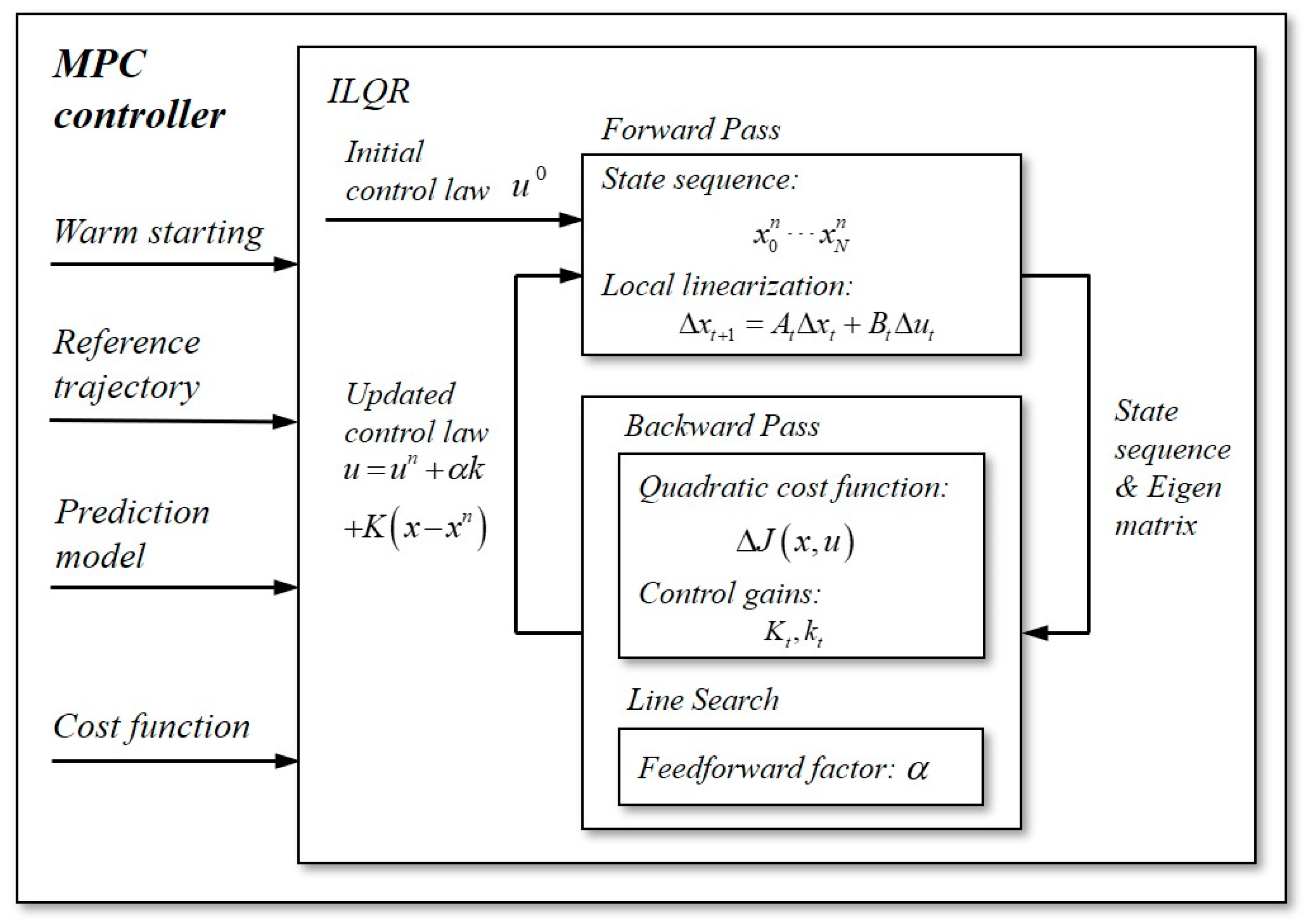
Based on the ILQR algorithm, we designed the MPC controller to realize finite horizon optimal control for the DVPUAV (please see Figure 15 and Algorithm 1). The longitudinal and lateral directional sub-controllers have the same control structure, in which the optimization computation in the inner layer is based on the ILQR algorithm, and the computational condition updating in the outer layer is based on MPC. The nonlinear optimization problem of the MPC controller takes the following form
where represent the state and input sequences, respectively, represent the state and input reference sequences, respectively, represent the state variables and inputs at moment, respectively, represents the constraint set of inputs.
- (1)
- State variables and Inputs
The state variables and inputs for the longitudinal sub-controller are and , respectively, while the state variables and inputs for the lateral directional sub-controller are and , respectively.
- (2)
- Constraints
One advantage of MPC over other control methods is that it allows explicit constraints. From the perspective of UAV physical constraints, the throttle of all groups of propulsion wings is in the range of , while the deflection angle of the blown flap is in the range of , that is, from to (). For this reason, in order to ensure sufficient attitude control capabilities for the DVPUAV, the constraints of inputs of the MPC controller are designed as follows
- (3)
- Warm starting
The MPC controller provides an input sequence as the initial control law for ILQR, which determines the convergence speed of ILQR. When MPC is run at high frequency, the input trajectories generated in adjacent time steps are usually close to each other. Therefore, the last controller could provide a good initialization for the next one.
- (4)
- Reference trajectory
The reference trajectory of the MPC controller is generated by the flight command , and it is continuously updated with the rolling optimization ().
- (5)
- Prediction model
Although the longitudinal control and lateral directional control are decoupled (as described in Section 3.2), the prediction models of both of them are complete system models as in Equation (46). What is more, the longitudinal sub-controller provides baseline inputs () for the lateral directional one, so, running the longitudinal sub-controller first is right in every computation step.
- (6)
- Cost function
The goal of the controller design is to act with the simplest inputs based on fast and accurate command tracking. The cost function is designed in a quadratic form,
where represents the deviation of a state from a desired one, represents the input, and are the weight matrices of terminal cost, state cost and input cost, respectively.
| Algorithm 1 Finite horizon optimal control for the DVPUAV | |
| 1: | Input |
| 2: | Warm starting: |
| 3: | Reference trajectory: |
| 4: | Output |
| 5: | Optimal control: |
| 6: | From virtual inputs to real inputs: |
| 7: | Repeat |
| 8: | Longitudinal sub-controller |
| 9: | Warm starting: |
| 10: | Reference trajectory: |
| 11: | Prediction model: Discrete form of Equation (46) |
| 12: | Cost function: |
| 13: | Run ILQR Obtain |
| 14: | Lateral directional sub-controller |
| 15: | Warm starting: |
| 16: | Reference trajectory: |
| 17: | Prediction model: Discrete form of Equation (46) |
| 18: | Cost function: |
| 19: | Run ILQR Obtain |
| 20: | Inputs integration |
| 21: | |
| 22: | Until terminal time |
4. Discussion and Analysis
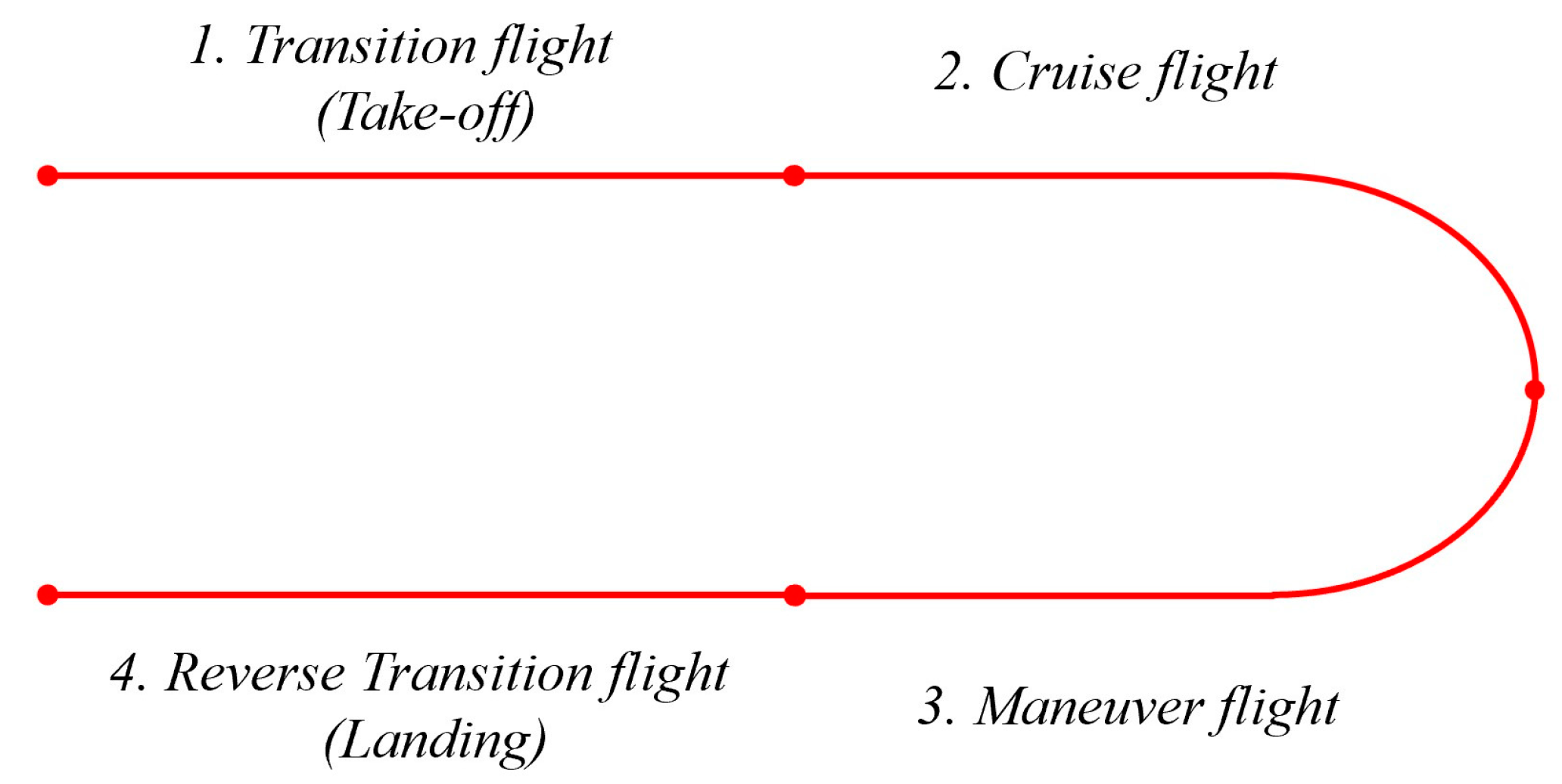
To verify the reliability and performance of the proposed control scheme (the DCFMPC, decoupling control framework + MPC controller), a flight simulation including multi-scenario tasks from takeoff to landing was carried out as Figure 16 shows. The task flow includes four types of flights: 1. Transition flight (Take-off)—2. Cruise flight—3. Maneuver flight—4. Reverse transition flight (Landing). The airspeeds of the ending point of the transition flight and the starting point of the reverse transition flight are both “critical speed”, that is, the minimum speed of fast mode, which is similar to the stall speed of conventional fixed-wing aircraft.
The state variables of the DVPUAV are , only a few of are vital for flight command design. The tracking for velocity and altitude obtains the most focus in longitudinal motion, while the tracking of the roll angle and the elimination of the sideslip angle are most important in lateral and directional motion. Therefore, the core tracking states are .
The control law parameters employed in this paper are given as follows: The horizon of control and prediction is , sample time is . The weights for state, input and terminal cost of longitudinal and lateral directional sub-controllers are shown in Table 1 and Table 2. Moreover, the control efficiency and response speed of the aerodynamic surface are better than the throttle of the propulsion wing, so the control gains of are bigger than .
In order to analyze the superiority of the DCFMPC, the GSPID (Gain scheduling Proportional-Integral-Derivative) widely used for VTOL aircraft is added as a comparison. The control framework of the GSPID is based on PX4 commercial flight control, but it also follows the decoupling of longitudinal and lateral directional control. The slow mode sub-PID controller is designed based on the hovering state, while the fast mode sub-controller is designed based on the cruising state, then, the two sub-controllers are mixed through a weight function.
The simulations were carried out based on matlab2022b, MathWorks (Natick, MA, USA) with the help of an Intel Core i7-1165g7 CPU with 16 GB of RAM. The DVPUAV has an overall weight of with cruise speed, the chord length of the front propulsion wing is and that of the rear propulsion wing is . Besides, the rotor diameter of the propulsion wing is with a maximum rotation speed of .
Simulation 1
Transition flight (Take-off)
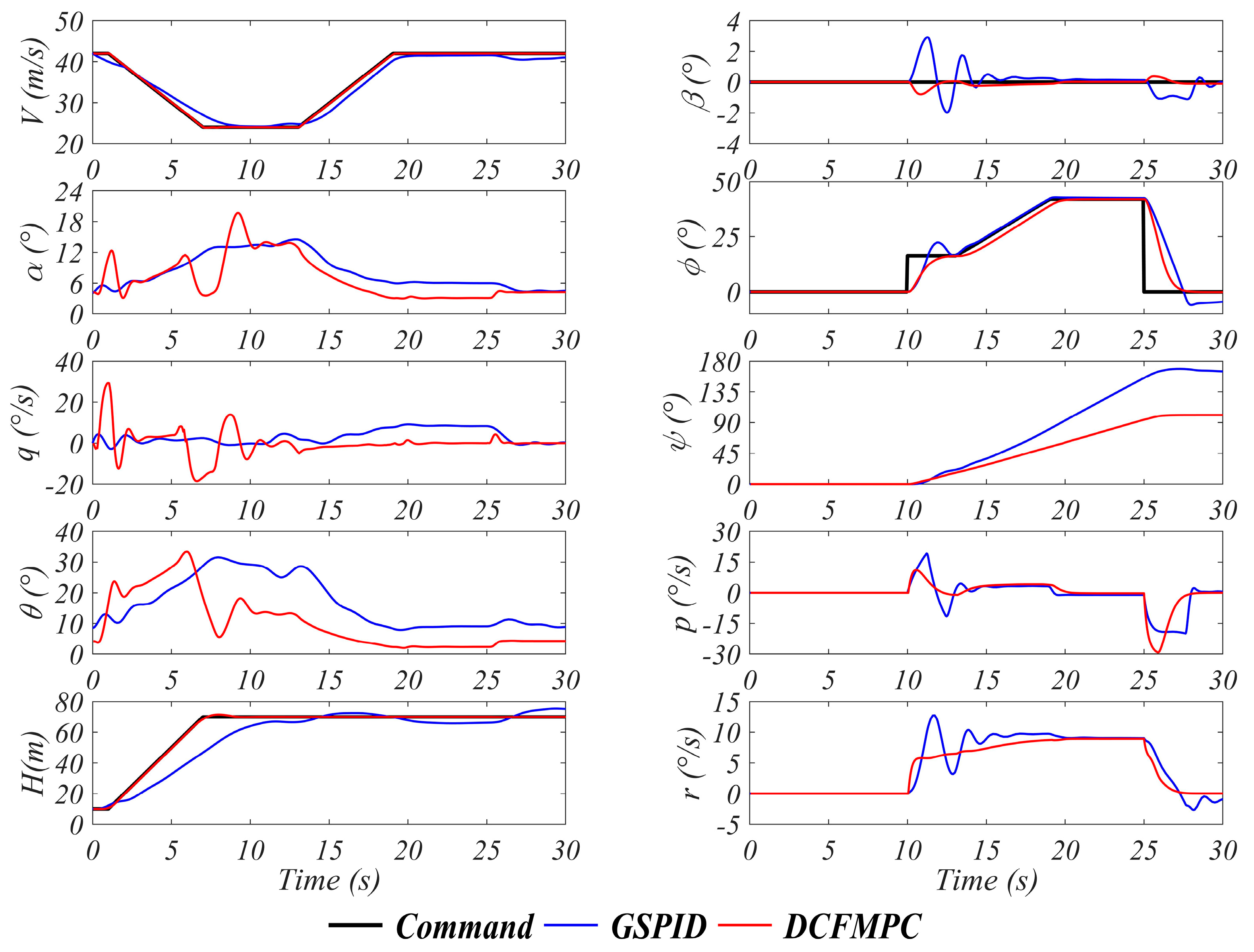
This simulation is conducted for the transition flight (takeoff) with the initial state . The flight command is designed to guide the DVPUAV to accelerate and climb uniformly until reaching a critical speed, then to level flight. Additionally, it provides a roll command at the moment from 10 s to 20 s to adjust the flight path and keep the sideslip angle command zero.
The DCFMPC has achieved satisfactory control effects in both longitudinal and lateral directional motions as Figure 17 shows. The GSPID has also achieved good tracking of airspeed and altitude. There is a small overshoot and no chatter in the simulation, indicating that the proportional gain of the GSPID is appropriate. The static error in the tracking process is basically zero, indicating that the integrator of the GSPID plays an important role in tracking. However, in terms of tracking speed and accuracy, the GSPID is inferior to the DCFMPC. This is because the GSPID controller is a mixture of slow mode and fast mode sub-controllers with weight function, which makes it difficult for the GSPID to always maintain the optimal scheduling effect. As a MIMO controller, the performance of the DCFMPC is naturally superior to the PID controller (SISO), when dealing with strongly nonlinear coupled systems (aerodynamic propulsion coupling, longitudinal and lateral coupling) and multiple states tracking scenarios. More importantly, based on the proposed dynamic model, the DCFMPC controller can not only obtain the current state of the UAV but also predict the future state, thereby solving the inputs through the internal ILQR algorithm, achieving fast and stable command tracking.
The DVPUAV is at a high pitch angle state during VTOL, overcoming gravity with system thrust (including rotor thrust and coupled aerodynamic forces from it), which brings new control problems. In kinematics, the rotation matrix between the Euler angle and the body angular velocity cannot be simplified as a diagonal matrix. In dynamics, there is an undeniable inertial coupling in the attitude motion. Besides, there is a strong aero-propulsion coupling during VTOL making the lateral directional coupling problem more complex. Therefore, in order to achieve a high-precision lateral directional control effect, it is necessary to cooperate with the lateral directional control channels. As Figure 17 shows, the DCFMPC exhibits better control performance than the GSPID in the lateral directional motion, and its advantage stems from the following two points. Firstly, the decoupling control framework adopts incremental inputs in lateral directional control, which can more finely manipulate each actuator compared to differential inputs, enabling actuators to achieve the best collaborative effect. Secondly, the DCFMPC performs well in roll angle tracking and sideslip angle elimination because of its prediction and optimization capabilities, and it has the capability to smooth and constrain inputs, thus achieving a comprehensive optimization of command tracking and input response.
As analyzed in Section 3.3, the DVPUAV has redundancy in longitudinal control and coupling in lateral directional control. For this reason, the input optimization is considered in the DCFMPC (please see the left four figures of Figure 18), which not only makes input change smoother but also makes throttle and deflection inputs (including baseline and longitudinal differential inputs) smaller than the GSPID. As shown in the right four figures of Figure 18, because of its incremental inputs, the DCFMPC has more flexible manipulation compared to the GSPID. Thanks to the collaborative manipulation of all actuators in the lateral directional control, more precise control effects have been achieved with a lower control input cost.
Simulation 2
Cruise flight
The second simulation is conducted for the cruise flight with the initial state . The flight command is designed to guide the DVPUAV to fly at cruise speed with the process of climbing and descending. Additionally, it leads the UAV to turn right first and then left, and provides a zero sideslip angle command.
In the cruise state (see Figure 19), the GSPID is not inferior to the DCFMPC. The GSPID only has a small overshoot during cruise flights, and based on coordinated turning, the UAV achieves great sideslip elimination while rolling. Therefore, for the DVPUAV cruise state, the GSPID is good enough to meet the control requirements. In fact, the characteristics of the DVPUAV in cruise states are basically consistent with those of traditional fixed wings, based on two reasons: 1. The DVPUAV is a static stability aircraft with good dynamic stability. 2. At the cruise state, the thrust demand is small, so the aero-propulsion coupling effect is very weak.
Therefore, the difficulty of control for the DVPUAV-type aircraft is not in the cruise state, but rather in the takeoff and landing stages with large attitude angles and a strong aero-propulsion coupling effect.
Simulation 3
Maneuver flight
The third simulation is conducted for maneuver flight with the initial state . The flight command is designed to guide the DVPUAV to accelerate and decelerate quickly with a rapid climb. Additionally, it leads the UAV to turn right with a constant radius and provides a zero sideslip angle command.
As Figure 20 shows, although the GSPID performs well in the cruise state, the tracking of the airspeed and altitude is not ideal in this extreme maneuver (for the case of unmanned aerial vehicles). On the one hand, the airspeed command decreases, leading to the plunge of the requirement of the throttle input, while the altitude command increases, causing an increased demand for the throttle input, which results in a conflict in the throttle input. On the other hand, the rapidly changing demand for head up makes the pitch manipulation capability of the DVPUAV close to the limit. Therefore, based on the above reasons, the longitudinal state tracking of the GSPID in this scenario is not satisfactory. The DCFMPC can utilize the future flight command to bring the longitudinal control ability of the UAV into full play, thus enabling the aircraft to respond in time to achieve good tracking of multiple states.
During constant radius turns in the range of 10~25 s, the DCFMPC performs slightly better than the GSPID, with almost no overshoot in roll angle tracking, and the sideslip angle close to zero at all times. However, in the range of 13~19 s, the DCFMPC is rarely inferior to the GSPID in the roll angle tracking. This is because the DCFMPC focuses on the optimization of the overall performance, and at this time, the DCFMPC has a better effect in eliminating the sideslip angle. Overall, the lateral directional control effect of the DCFMPC is still better than that of the GSPID in the entire maneuver process.
Simulation 4
Reverse transition flight (Landing)
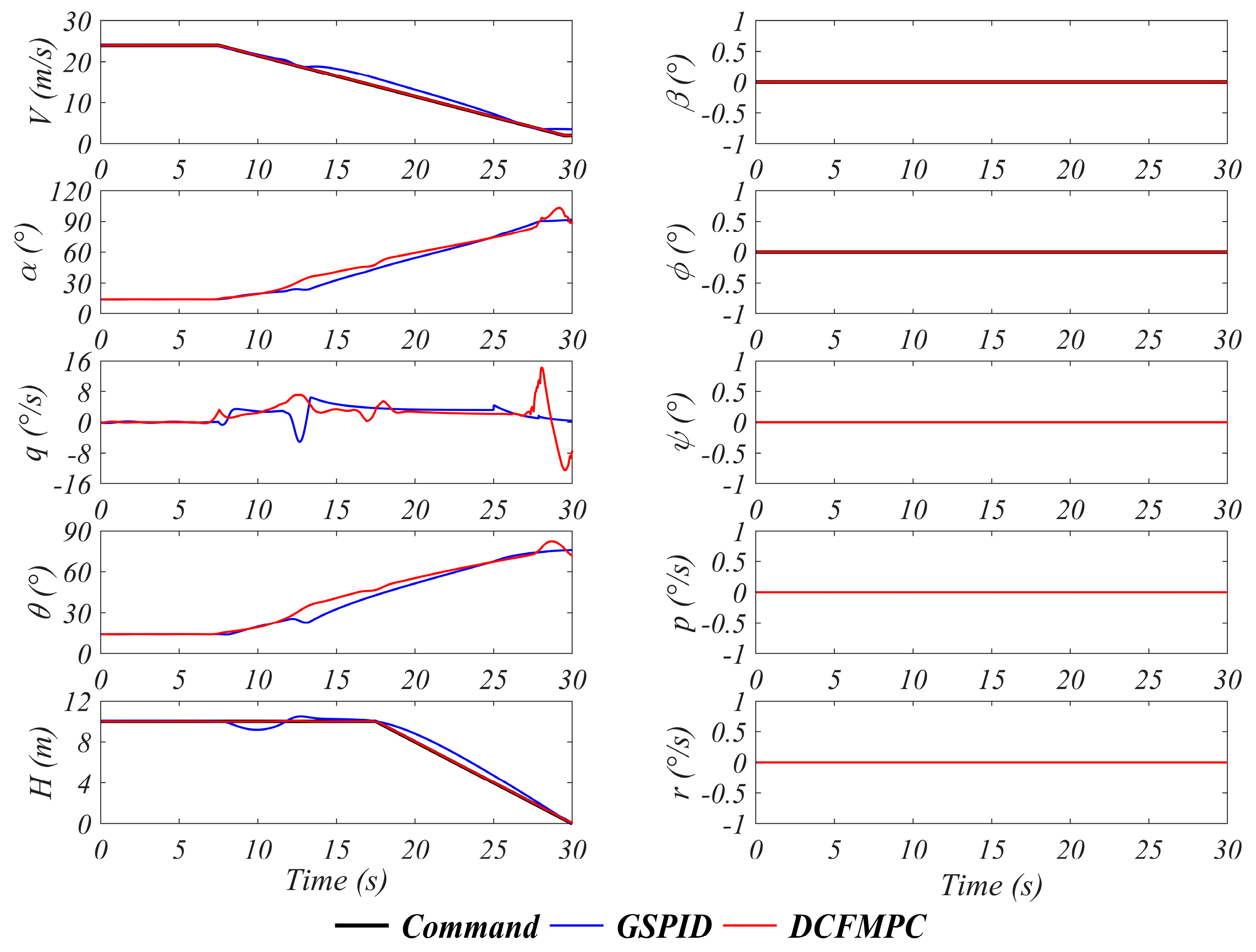
This simulation is conducted for reverse transition flight (landing) with the initial state . The flight command is designed to guide the DVPUAV to decelerate and descend until touching the ground. Additionally, keep the roll angle and sideslip angle command zero.
In fact, the reverse transition flight (landing) is more difficult and dangerous than the transition flight (takeoff). From the perspective of flight dynamics, the DVPUAV changes from stability to instability during the reverse transition flight, so, there is a higher performance requirement for the control system. During the landing process, except for the adjustment of position and attitude before touchdown, lateral maneuvering should be avoided as much as possible.
In Figure 21, from the 7.5 s moment, the UAV begins to decelerate; however, the altitude tracking error based on the GSPID fluctuates between 7.5 and 17.5 s. This is because although the fast mode sub-controller of the GSPID is designed based on the Total Energy Control System (TECS), the inputs of throttle and deflection are still independent of each other, so there is a competitive relationship between the control channels. During this period, the DCFMPC performed great in both airspeed tracking and altitude tracking, reflecting the advantage of control optimization based on state space. After 17.5 s, the UAV begins to descend, accompanied by a further decrease in airspeed. However, during this process, the attack angle of the DVPUAV persistently climbs or even exceeds 90°, resulting in non-monotonicity and strong nonlinearity in the aerodynamics, which brings a huge challenge to the control system, leading to an obvious tracking error of the GSPID. On the contrary, it can be seen that the pitch angle and pitch angular velocity response based on the DCFMPC are more flexible. This is not the chattering phenomenon that occurs in the sliding mode control (SMC), but the rapid response made based on its predictive optimization ability at this time, which enables the DVPUAV to fully exert its control potential and achieve excellent airspeed and altitude tracking.
The overall input response of the DCFMPC and the GSPID are consistent as shown in Figure 22. However, the input response of the DCFMPC is faster and smoother, bringing less burden to actuators. During the landing process, the throttle input continuously climbs, indicating that the fast mode is more energy-friendly compared to the slow mode. Therefore, for VTOL aircraft, on the basis of ensuring a safe and smooth transition, shortening the transition time is beneficial for saving energy to increase the flight range or reduce the structure weight.
It is worth mentioning that coupling in dynamics is an inherent property of the system, including but not limited to motion coupling, inertial coupling, and aerodynamic coupling. The control system cannot forcibly change the dynamic coupling, and can only perform partial feedforward compensation and feedback to eliminate tracking errors. Therefore, if the control system can obtain a reliable dynamic model, has the capability to predict future states (enhance feedforward compensation ability), simplify control logic and has the capability to coordinate global inputs (enhance feedback control performance), it is beneficial for improving control performance.
Implementation
In order to further test the control performance under the uncertainty [39,40] of the proposed DCFMPC controller, more simulations are taken for cruise flight and reverse transition flight (landing) with uncertain disturbances. System uncertainty acts on the DVPUAV by the external forces and moments disturbance in the form of Gaussian white noise. The noise variance of forces and moments are selected as and , respectively, according to their characteristics.
Simulation 5
Cruise flight with uncertainty
This simulation is conducted for cruise flight with the initial state under uncertainty. The flight command is consistent with simulation 2.
As Figure 21 shows, the GSPID controller has a comparable control accuracy to the DCFMPC in simulation 2. However, when there are continuous random forces and moments disturbances, the control accuracy of the GSPID significantly decreases in Figure 23, especially in airspeed tracking and altitude tracking. On the contrary, the DCFMPC has shown good anti-disturbance capability, and its command tracking accuracy is still satisfactory (see Figure 23). In the sub-figures of roll angular velocity, pitch angular velocity, and yaw angular velocity, both the DCFMPC and the GSPID exhibit high-frequency chattering, which reflects that they desire to overcome the effects of interference through rapid response. Thanks to the ability of rolling optimization and making full use of the dynamic model, the DCFMPC enables the state response of the UAV to be smoother while achieving high-precision command tracking.
Simulation 6
Reverse transition flight(landing) with uncertainty
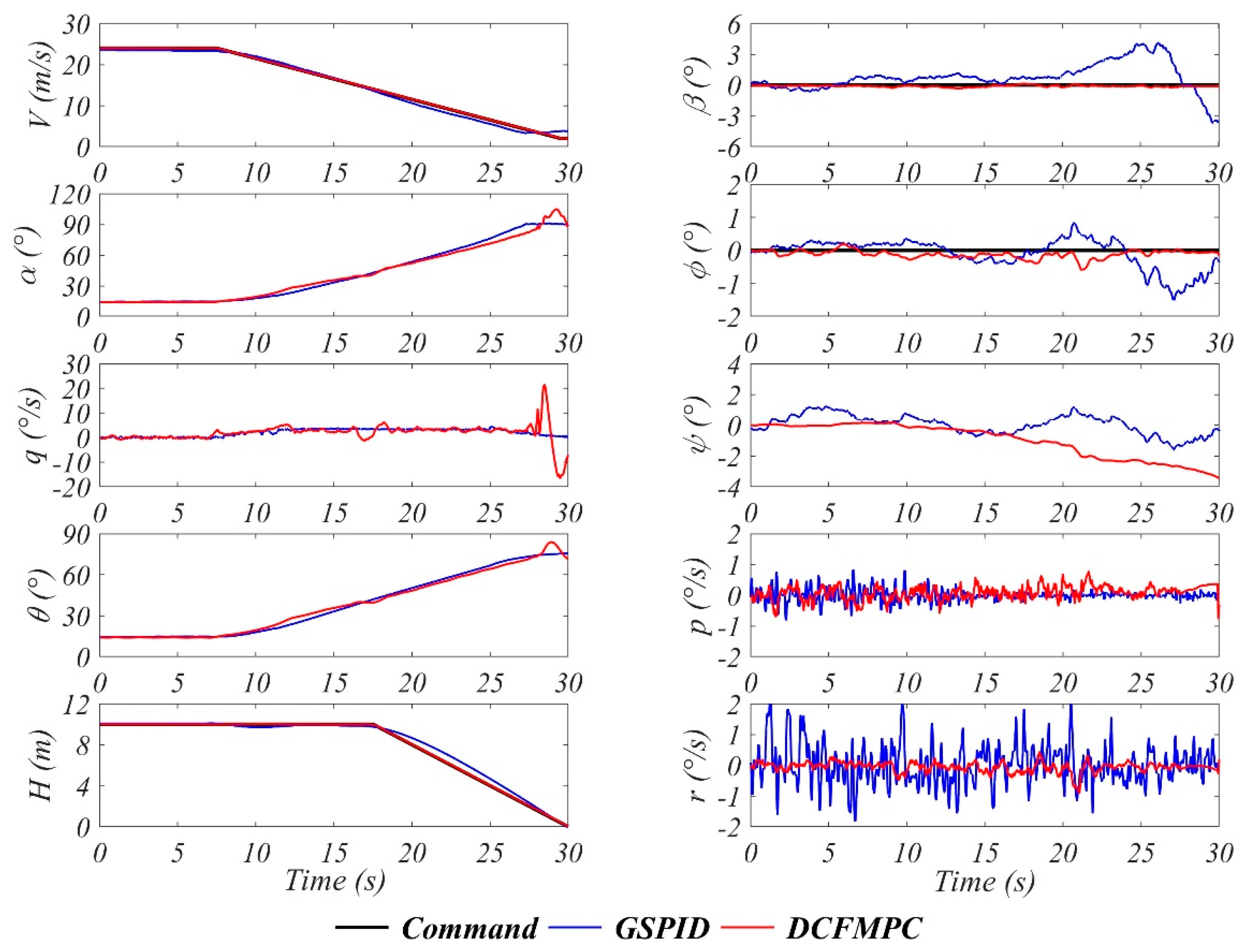
This simulation is conducted for a reverse transition flight (landing) with the initial state under uncertainty. The flight command is designed to guide the DVPUAV to decelerate and descend until it touches the ground, which is the same as in simulation 4.
Although the longitudinal control effect of the GSPID in this simulation (see Figure 24) seems to be close to that in simulation 4, it does not necessarily mean that the GSPID has a strong anti-disturbance capability in the landing process. It can only be explained that the control effect of the GSPID has not further deteriorated significantly. As Figure 24 shows, the DCFMPC still demonstrates good command tracking capability in longitudinal control. Compared with Figure 21, there is a high-frequency chatting of pitch rate, and the response amplitude of pitch rate increases in the range of 27~30s when the aircraft is about to land, indicating that the MPC controller is trying to overcome the uncertainty. In terms of lateral directional control, although the DCFMPC performs better than the GSPID, its control accuracy has also slightly decreased compared to simulation 4. After all, feedback-based control can only eliminate an error after it occurs. To enhance the anti-disturbance ability of the controller, future research intends to use a disturbance observer for uncertainty compensation. Overall, the DCFMPC can deal with uncertainties more effectively than the GSPID.
5. Conclusions
In this paper, the DVPUAV is introduced with good aerodynamic performance and TVC capability, which could realize not only S/VTOL but relatively high-speed cruise. This type of aircraft is a popular research topic at present with great value in theoretical research and engineering application.
The proposed APCM with analytical expression realizes a clear description of the complex aero-propulsion coupling effect by an extremely simplified mechanical relationship which has the capability to meet the dual requirements of reliability and real-time performance in flight dynamics and control. Thus, it is a potential ideal model for flight dynamics and flight control. Moreover, the characteristic of the distributed layout of UAVs is considered in modeling, so the proposed nonlinear dynamic model can well describe the dynamic behavior of the DVPUAV.
The proposed control framework realizes the decoupling of longitudinal and lateral control, as well as the decoupling of roll and yaw control. The MPC controller based on the decoupling control framework has successfully dealt with the nonlinear control problem of the DVPUAV so that the DVPUAV achieves excellent command tracking from takeoff to landing. Compared to a traditional VTOL controller (the GSPID), the DCFMPC has better control performance with fast and smooth input responses. It is worth mentioning that not only the unification of longitudinal and lateral directional sub-controllers but also the unification of the controller of the full flight envelope is achieved in our work.
In the future, we mainly plan to focus on the following two aspects of work. Firstly, we will conduct vehicle-mounted and wind tunnel experiments to calibrate and validate the APCM based on more reliable data. Secondly, we will carry out indoor suspension and outdoor flight experiments of UAVs to test the effectiveness of the control method in real flight.
Author Contributions
Conceptualization, J.X. and Z.Z.; methodology, J.X.; software, J.X.; validation, J.X.; formal analysis, J.X.; investigation, J.X.; resources, Z.Z.; data curation, Z.Z.; writing—original draft preparation, J.X.; writing—review and editing, J.X.; visualization, J.X.; supervision, Z.Z.; project administration, Z.Z.; funding acquisition, Z.Z. All authors have read and agreed to the published version of the manuscript.
Funding
This research was funded by National Defense Fund, grant number 2021-JCJQ-JJ-0805.
Institutional Review Board Statement
Not applicable.
Informed Consent Statement
Not applicable.
Data Availability Statement
Sample data available on request.
Conflicts of Interest
The authors declare no conflicts of interest.
Nomenclature
| Velocity of free-stream | |
| Velocity of exit flow | |
| Velocity of far field flow | |
| Attack angle of propulsion wing | |
| Attack angle of blown flap | |
| Deflection angle of the blown flap | |
| Downwash angle of exit flow | |
| Span of propulsion wing unit | |
| Chord length of upper surface of shroud | |
| Chord length of lower surface of shroud | |
| Chord length of blown flap | |
| Equivalent angle of the upper lip of shroud | |
| Equivalent angle of the lower lip of shroud | |
| Axial distance from the lower lip to rotor disc | |
| Axial distance from exit station to rotor disc | |
| Radius of lower lip | |
| Radius of upper lip | |
| Radius of rotor | |
| Radius of rotor station (camber line) | |
| Radius of exit station | |
| Nondimensionalized parameter of | |
| Nondimensionalized parameter of | |
| Pressure before the rotor disc | |
| Pressure after the rotor disc | |
| Air Density | |
| Axial component of airspeed | |
| Axial velocities of rotor station | |
| Axial velocities of far field | |
| Thrust of rotor | |
| Thrust of shroud | |
| Total thrust of rotor and shroud system | |
| System thrust augmentation coefficient | |
| Axial force augmentation coefficient of shroud | |
| Normal force augmentation coefficient of shroud | |
| Dimensionless axial velocity on the centerline | |
| Dimensionless axial induced velocity by rotor disc | |
| Dimensionless axial induced velocities by airfoil camber of shroud (rotor station) | |
| Dimensionless axial induced velocities by airfoil camber of shroud (lower lip) | |
| Dimensionless axial induced velocity by area | |
| Dimensionless normal velocity | |
| Dimensionless normal velocity on the centerline | |
| Dimensionless normal induced velocity by free-stream | |
| Dimensionless normal induced velocity by airfoil camber of shroud (lower lip) | |
| Mutual repulsion effect of airflow | |
| Circulation term related to rotor disc | |
| circulation term related to vortexes of shroud (rotor station) | |
| circulation term related to vortexes of shroud (lower lip) | |
| Cross-sectional area of rotor station | |
| Cross-sectional area of exit station | |
| Normal force of shroud | |
| Axial velocity of exit flow | |
| Normal velocity of exit flow | |
| Lift coefficient at zero attack angle of isolated shroud | |
| Lift curve slope of isolated shroud | |
| Zero lift drag coefficient of isolated shroud | |
| Induced drag factor of isolated shroud | |
| Term related to maximum lift coefficient of isolated shroud stall model | |
| Term related to maximum drag coefficient of isolated shroud stall model | |
| Slew factor of laminal and stall models of isolated shroud | |
| Slew attack angle | |
| Slew rate | |
| Reference area of shroud | |
| Lift of isolated shroud | |
| Drag of isolated shroud | |
| Lateral force of isolated shroud | |
| Sideslip angle | |
| Deflection angle of wake | |
| Reaction force generated by jet deflection caused by the blown flap | |
| Blowing momentum coefficient | |
| Reference area of shroud | |
| Aerodynamic derivatives of blown flap related to free stream | |
| Induced drag factor of blown flap | |
| Lift of blown flap | |
| Drag of blown flap | |
| Propulsion wing unit coordinate system | |
| Coordinate system of the front propulsion wing | |
| Coordinate system of the rear propulsion wing | |
| Body coordinate system | |
| Inertial coordinate system | |
| Forces on the shroud in | |
| Forces on the blown flap in | |
| Forces of propulsion wing unit | |
| Pitch moment of propulsion wing unit | |
| Reference point of propulsion wing unit | |
| Distance between action position of to the | |
| Distance between action position of to the | |
| Rotation transformation matrix from to | |
| Rotation transformation matrix from to | |
| Relative angle between and | |
| Location throttle and deflection input of propulsion wing | |
| Front propulsion wing groups number | |
| Rear propulsion wing groups number | |
| Longitudinal distance parameters of DVPUAV | |
| Lateral distance parameters of DVPUAV | |
| Vertical distance parameters of DVPUAV | |
| Aerodynamic forces and moments of fuselage and winglets | |
| Gravity of DVPUAV | |
| Mass of DVPUAV | |
| Moment of inertia of DVPUAV | |
| Angular velocity vector | |
| Velocity vector | |
| Throttle inputs distribution on DVPUAV | |
| Deflection inputs distribution on DVPUAV | |
| Baseline inputs | |
| Longitudinal differential inputs | |
| Lateral directional increment inputs | |
| Flight state of UAV | |
| Flight command of UAV | |
| Control input | |
| System output | |
| State sequence | |
| Input sequence | |
| Number of knots | |
| Discrete moment | |
| State variables at moment | |
| Inputs at moment | |
| Gradient and Hessian matrices of the cost function | |
| First derivation of dynamics about state and input | |
| Reference state sequence | |
| Reference input sequence | |
| Constraint set of inputs | |
| State variables for longitudinal sub-controller | |
| Inputs for longitudinal sub-controller | |
| State variables for lateral sub-controller | |
| Inputs for lateral sub-controller | |
| Airspeed of DVPUAV | |
| Flight altitude | |
| Path angle | |
| Roll angle | |
| Pitch angle | |
| Yaw angle | |
| Roll rate | |
| Pitch rate | |
| Yaw rate | |
| Reference state at moment | |
| Deviation of a state from a desired one at moment | |
| Weight matrix of terminal cost | |
| Weight matrix of state cost | |
| Weight matrix of input cost | |
| Horizon of control and prediction | |
| Sample time |
References
- Pornet, C.; Isikveren, A.T. Conceptual design of hybrid-electric transport aircraft. Prog. Aerosp. Sci. 2015, 79, 114–135. [Google Scholar] [CrossRef]
- Baskaran, P.; Corte, B.D.; van Sluis, M.; Rao, A.G. Aeropropulsive Performance Analysis of Axisymmetric Fuselage Bodies for Boundary-Layer Ingestion Applications. AIAA J. 2022, 60, 1592–1611. [Google Scholar] [CrossRef]
- Kim, H.D.; Perry, A.T.; Ansell, P.J. A review of distributed electric propulsion concepts for air vehicle technology. In Proceedings of the 2018 AIAA/IEEE Electric Aircraft Technologies Symposium, Cincinnati, OH, USA, 12–14 July 2018; AIAA: Reston, VA, USA, 2018. [Google Scholar]
- Perry, A.T.; Timothy, B.; Phillip, J.A. Aeropropulsive Coupling Effects on a General-Aviation Aircraft with Distributed Electric Propulsion. J. Aircr. 2020, 58, 1351–1363. [Google Scholar] [CrossRef]
- Uranga, A.; Drela, M.; Greitzer, E.M.; Hall, D.K.; Titchener, N.A.; Lieu, M.K.; Siu, N.M.; Casses, C.; Huang, A.C.; Gatlin, G.M.; et al. Boundary Layer Ingestion Benefit of the D8 Transport Aircraft. AIAA J. 2017, 55, 3693–3708. [Google Scholar] [CrossRef]
- Wang, K.; Zhou, Z.; Fan, Z.; Guo, J. Aerodynamic design of tractor propeller for high-performance distributed electric propulsion aircraft. Chin. J. Aeronaut. 2021, 35, 20–35. [Google Scholar] [CrossRef]
- Mohamed, A.; Eike, S. Aero-propulsive interaction model for conceptual distributed propulsion aircraft design. Aircr. Eng. Aerosp. Technol. 2022, 94, 948–964. [Google Scholar]
- Zhang, X.; Zhang, W.; Li, W.; Zhang, X.; Lei, T. Experimental research on aero-propulsion coupling characteristics of a distributed electric propulsion aircraft. Chin. J. Aeronaut. 2023, 36, 201–211. [Google Scholar] [CrossRef]
- Gohardani, A.S. A synergistic glance at the prospects of distributed propulsion technology and the electric aircraft concept for future unmanned air vehicles and commercial/military aviation. Prog. Aerosp. Sci. 2013, 57, 25–70. [Google Scholar] [CrossRef]
- Li, Z.Y.; Liu, Y.D.; Zhou, W.W. Lift augmentation potential of the circulation control wing driven by sweeping jets. AIAA J. 2022, 60, 1–22. [Google Scholar] [CrossRef]
- Ducard, G.J.J.; Allensoach, M. Review of designs and flight control techniques of hybrid and convertible VTOL UAVs. Aerosp. Sci. Technol. 2021, 118, 107035. [Google Scholar] [CrossRef]
- Ugwueze, O.; Statheros, T.; Horri, N.; Bromfield, M.A.; Simo, J. An Efficient and Robust Sizing Method for eVTOL Aircraft Configurations in Conceptual Design. Aerospace 2023, 10, 311. [Google Scholar] [CrossRef]
- Rostami, M.; Bardin, J.; Neufeld, D.; Chung, J. EVTOL Tilt-Wing Aircraft Design under Uncertainty Using a Multidisciplinary Possibilistic Approach. Aerospace 2023, 10, 718. [Google Scholar] [CrossRef]
- Rohr, D.; Studiger, M.; Stastny, T.; Lawrance, N.R.J.; Siegwart, R. Nonlinear model predictive velocity control of a VTOL tiltwing UAV. IEEE Robot. Autom. Lett. 2021, 6, 5776–5783. [Google Scholar] [CrossRef]
- Xia, J.Y.; Zhou, Z. Model Predictive Control Based on ILQR for Tilt-propulsion UAV. Aerospace 2022, 9, 688. [Google Scholar] [CrossRef]
- Liu, N.; Cai, Z.; Zhao, J.; Wang, Y. Predictor-based model reference adaptive roll and yaw control of a quad-tiltrotor UAV. Chin. J. Aeronaut. 2020, 33, 282–295. [Google Scholar] [CrossRef]
- Ahmed, A.M.; Katupitiya, J. Modeling and control of a novel vectored-thrust quadcopter. J. Guid. Control Dyn. 2021, 44, 1399–1409. [Google Scholar] [CrossRef]
- Bauersfeld, L.; Spannagl, L.; Ducard, G.J.J.; Onder, C.H. MPC Flight Control for a Tilt-rotor VTOL Aircraft. IEEE Trans. Aerosp. Electron. Syst. 2021, 57, 2395–2409. [Google Scholar] [CrossRef]
- Mike, A.; Guillaume, J.J.D. Nonlinear model predictive control and guidance for a propeller-tilting hybrid unmanned air vehicle. Automatica 2021, 132, 109790. [Google Scholar]
- Bauersfeld, L.; Ducard, G. Fused-PID Control for Tilt-Rotor VTOL Aircraft. In Proceedings of the 2020 28th Mediterranean Conference on Control and Automation (MED), Saint-Raphaël, France, 15–18 September 2020. [Google Scholar]
- Rostami, M.; Chung, J.; Park, H.U. Design optimization of multi-objective proportional-integral-derivative controllers for enhanced handling quality of a twin-engine, propeller-driven airplane. Adv. Mech. Eng. 2020, 12, 1687814020923178. [Google Scholar] [CrossRef]
- Mayne, D.Q.; Rawlings, J.B.; Rao, C.V.; Scokaert, P.O.M. Constrained model predictive control: Stability and optimality. Automatica 2000, 36, 789–814. [Google Scholar] [CrossRef]
- Budhiraja, R.; Carpentier, J.; Mastalli, C.; Mansard, N. DDP for multi-phase rigid contact dynamics. In Proceedings of the IEEE-RAS 18th International Conference on Humanoid Robots (Humanoids), Beijing, China, 6–9 November 2018. [Google Scholar]
- Bellman, R.R. Dynamic programming. Science 1966, 153, 34–37. [Google Scholar] [CrossRef]
- Tassa, Y.; Mansard, N.; Todorov, E. Control-Limited Differential Dynamic Programming. In Proceedings of the IEEE International Conference on Robotics & Automation (ICRA), Hong Kong, China, 29 September 2014. [Google Scholar]
- Grandia, R.; Farshidian, F.; Ranftl, R.; Hutter, M. Feedback MPC for Torque-Controlled Legged Robots. In Proceedings of the IEEE/RSJ International Conference on Intelligent Robots and Systems (IROS), Macau, China, 3–8 November 2019. [Google Scholar]
- Liu, Z.; Yang, T.; Li, Z.; Li, Z. Automatic landing trajectory control of aircraft based on Iterative-LQR algorithm. In Proceedings of the 2022 9th International Forum on Electrical Engineering and Automation (IFEEA), Zhuhai, China, 4–6 November 2022. [Google Scholar]
- Sgueglia, A.; Schmollgruber, P.; Bartoli, N.; Atinault, O.; Benard, E.; Morlier, J. Exploration and sizing of a large passenger aircraft with distributed ducted electric fans. In Proceedings of the 2018 AIAA Aerospace Sciences Meeting, Kissimmee, FL, USA, 8–12 January 2018; AIAA: Reston, VA, USA, 2018; p. 1745. [Google Scholar]
- Beckers, M.F.; Schollenberger, M.; Lutz, T.; Bongen, D.; Radespiel, R.; Florenciano, J.L.; Funes-Sebastian, D.E. Numerical Investigation of High-Lift Propeller Positions for a Distributed Propulsion System. J. Aircr. 2023, 60, 995–1006. [Google Scholar] [CrossRef]
- Werle, M.J. Analytical model for ring-wing propulsor thrust augmentation. J. Aircr. 2020, 57, 901–913. [Google Scholar] [CrossRef]
- McCormick, B.W. Aerodynamics of V/STOL Flight; Courier Corporation: North Chelmsford, MA, USA, 1999. [Google Scholar]
- Werle, M.J. Aerodynamic Loads and Moments on Axisymmetric Ring-Wing Ducts. AIAA J. 2014, 52, 2359–2364. [Google Scholar] [CrossRef]
- Werle, M.J. Analytical Model for Ring-Wing Propulsors at Angle of Attack. J. Aircr. 2022, 59, 1351–1362. [Google Scholar] [CrossRef]
- ESDU. Aircraft Forces due to Interference between a Jet Efflux and a Slotted Flap; ESDU: Reston, VA, USA, 1982. [Google Scholar]
- Jakobsson, B. Definition and Measurement of Jet Engine Thrust. J. R. Aeronaut. Soc. 1951, 55, 226–243. [Google Scholar] [CrossRef]
- Beard, R.W.; McLain, T.W. Small Unmanned Aircraft: Theory and Practice; Princeton University Press: Princeton, NJ, USA, 2012. [Google Scholar]
- Zhong, J.Y.; Wang, C. Transition characteristics for a small tail-sitter unmanned aerial vehicle. Chin. J. Aeronaut. 2021, 34, 220–236. [Google Scholar] [CrossRef]
- Liu, N.; Cai, Z.; Wang, Y.; Zhao, J. Fast level-flight to hover mode transition and altitude control in tiltrotor’s landing operation. Chin. J. Aeronaut. 2021, 34, 181–193. [Google Scholar] [CrossRef]
- Ullah, S.; Mehmood, A.; Khan, Q.; Rehman, S.; Iqbal, J. Robust Integral Sliding Mode Control Design for Stability Enhancement of Under-actuated Quadcopter. Int. J. Control Autom. Syst. 2020, 18, 1671–1678. [Google Scholar] [CrossRef]
- Ullah, S.; Khan, Q.; Zaidi, M.M.; Hua, L.-G. Neuro-adaptive non-singular terminal sliding mode control for distributed fixed-time synchronization of higher-order uncertain multi-agent nonlinear systems. Inf. Sci. 2024, 659, 120087. [Google Scholar] [CrossRef]
Figure 1.
General layout of the DVPUAV.
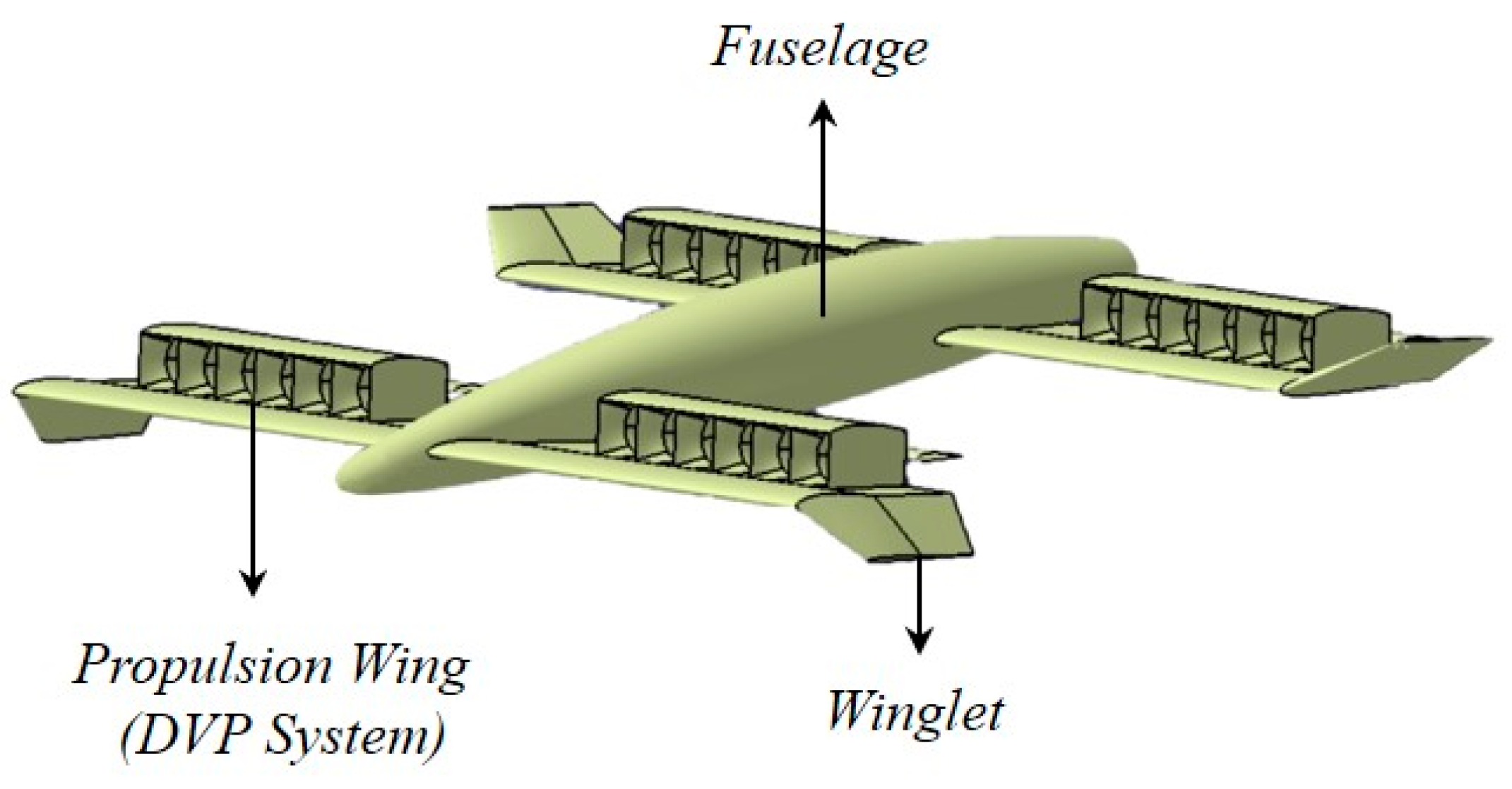
Figure 2.
Propulsion wing prototype.

Figure 3.
Computational logic of the aero-propulsion coupling model.

Figure 4.
Diagram of rotor and shroud.
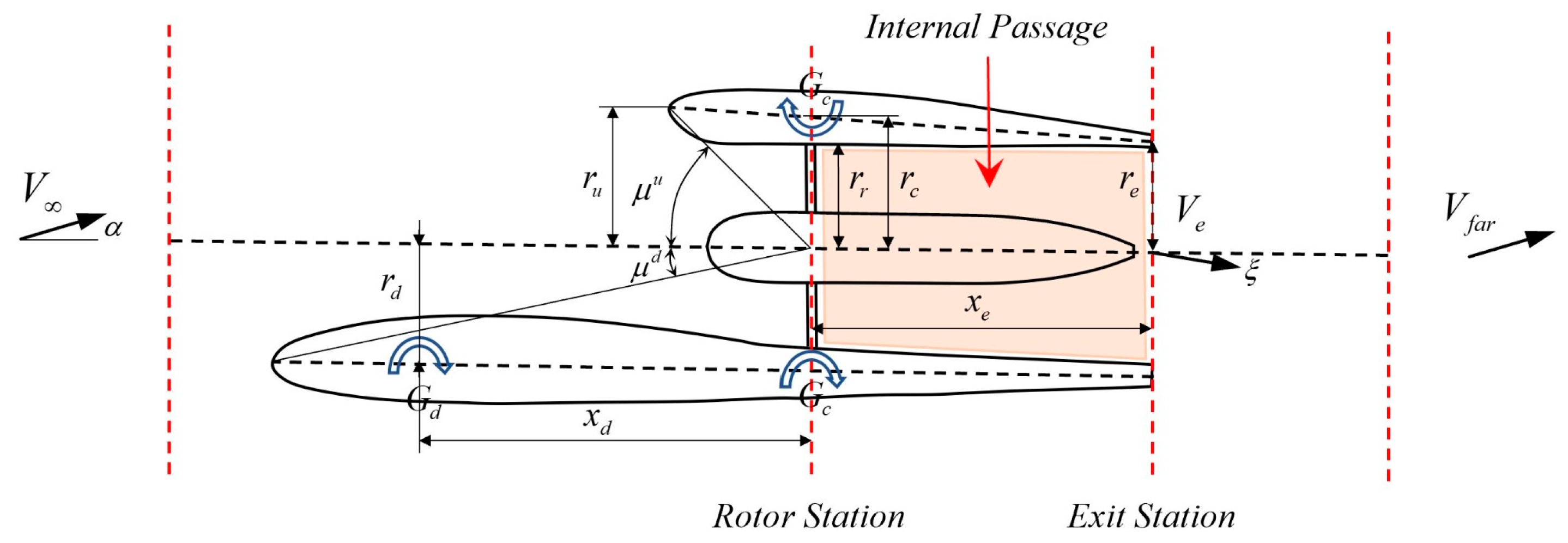
Figure 5.
Four components of centerline velocity.
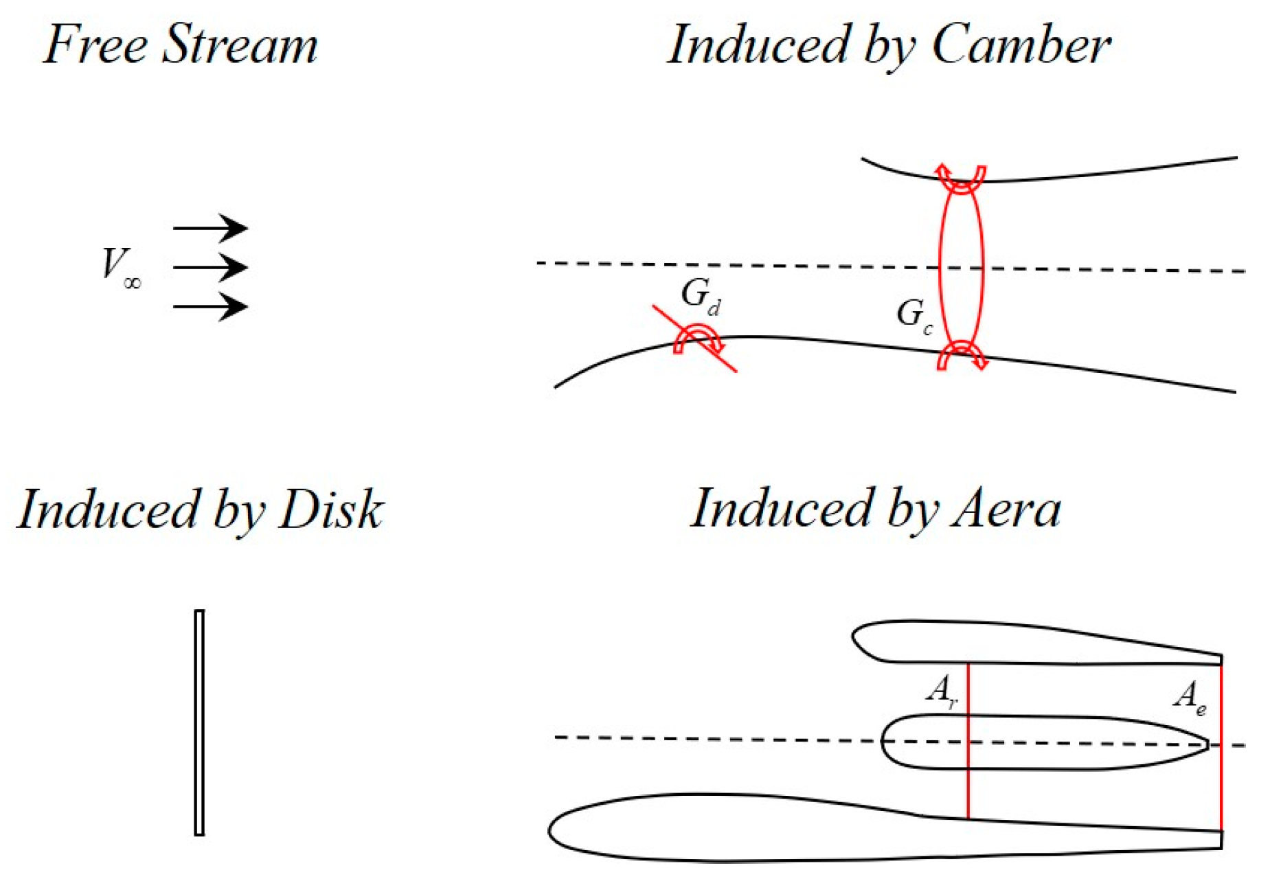
Figure 6.
Forces of propulsion wing.
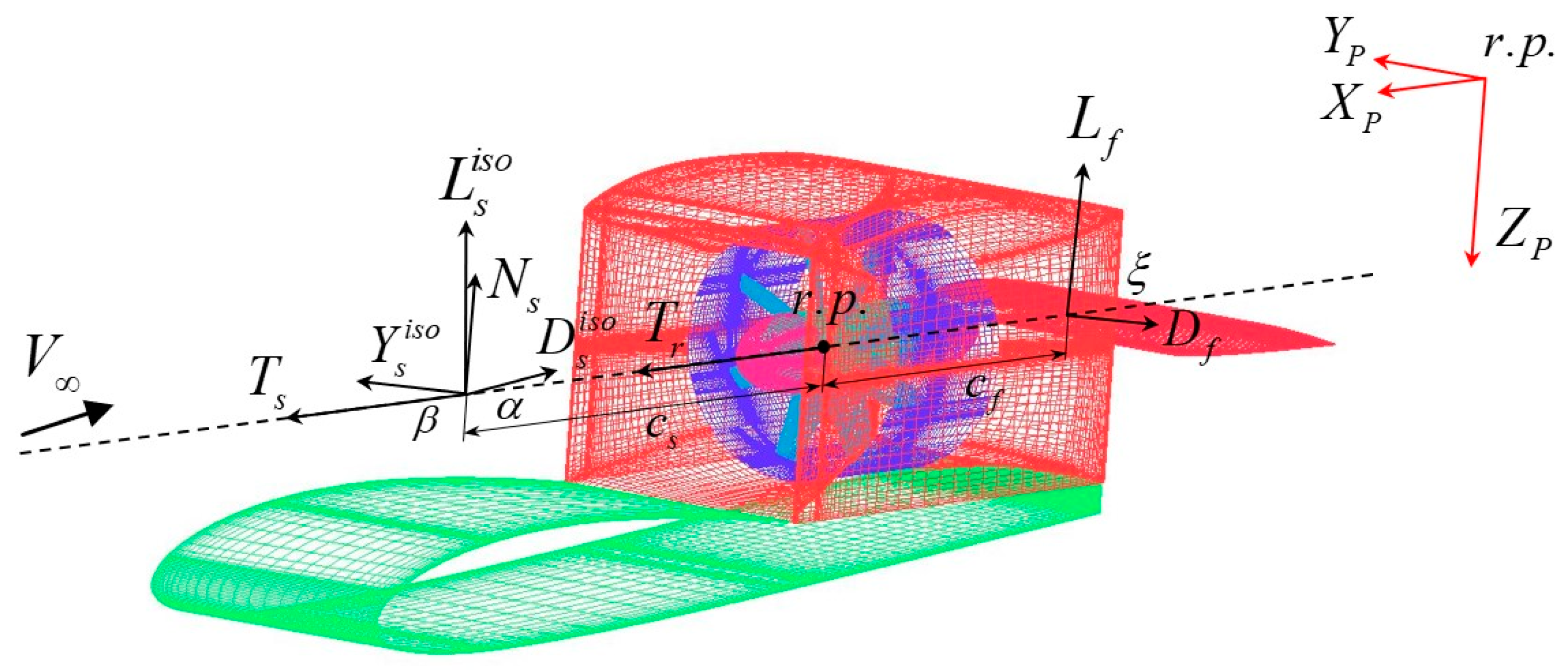
Figure 7.
Vertical and side view of the DVPUAV. (a) Vertical view (b) Side view.
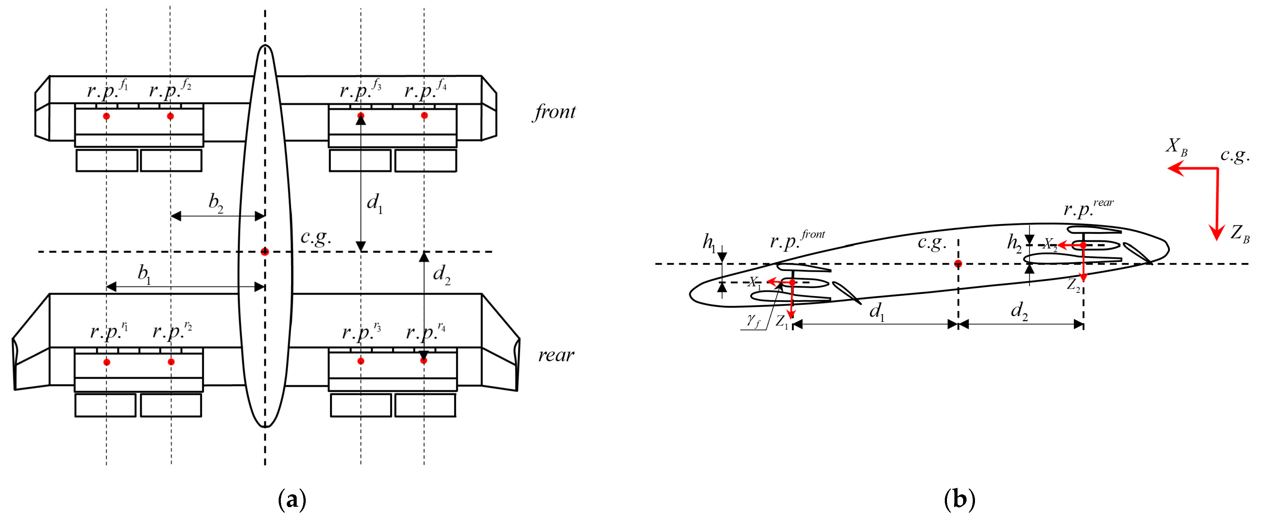
Figure 8.
Slow and fast modes of the DVPUAV.
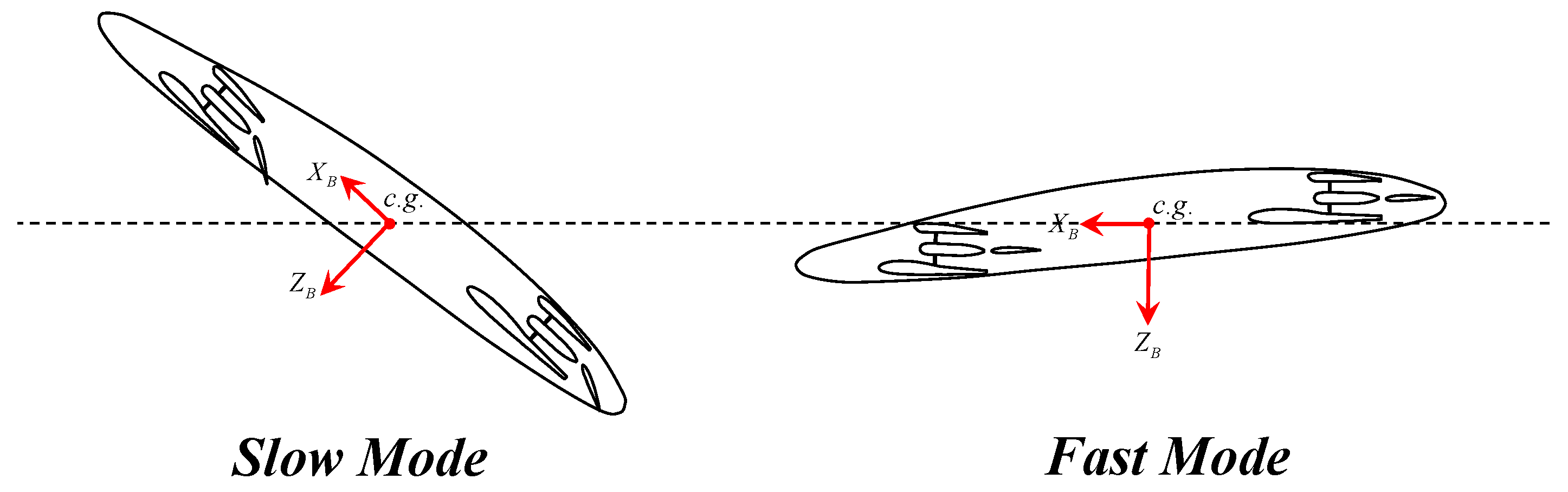
Figure 9.
Diagram of Takeoff and landing process of the DVPUAV. (a) Takeoff process (b) Landing process.
Figure 9.
Diagram of Takeoff and landing process of the DVPUAV. (a) Takeoff process (b) Landing process.

Figure 10.
Inputs of the DVPUAV.
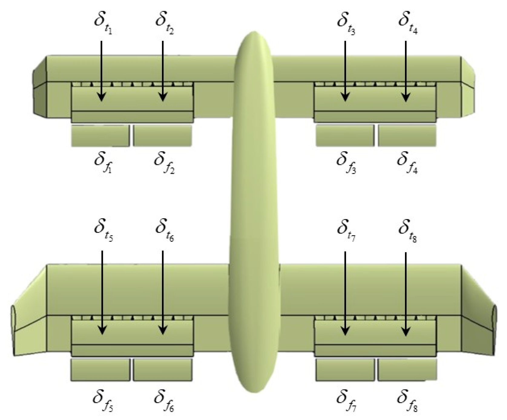
Figure 11.
Longitudinal and lateral directional inputs of the DVPUAV.

Figure 12.
Coupling of roll and yaw control. (a) Effect of only throttle differential control (b) Effect of only deflection differential control.
Figure 12.
Coupling of roll and yaw control. (a) Effect of only throttle differential control (b) Effect of only deflection differential control.

Figure 13.
Ideal effect of lateral directional control. (a) Roll control (b) Yaw control.
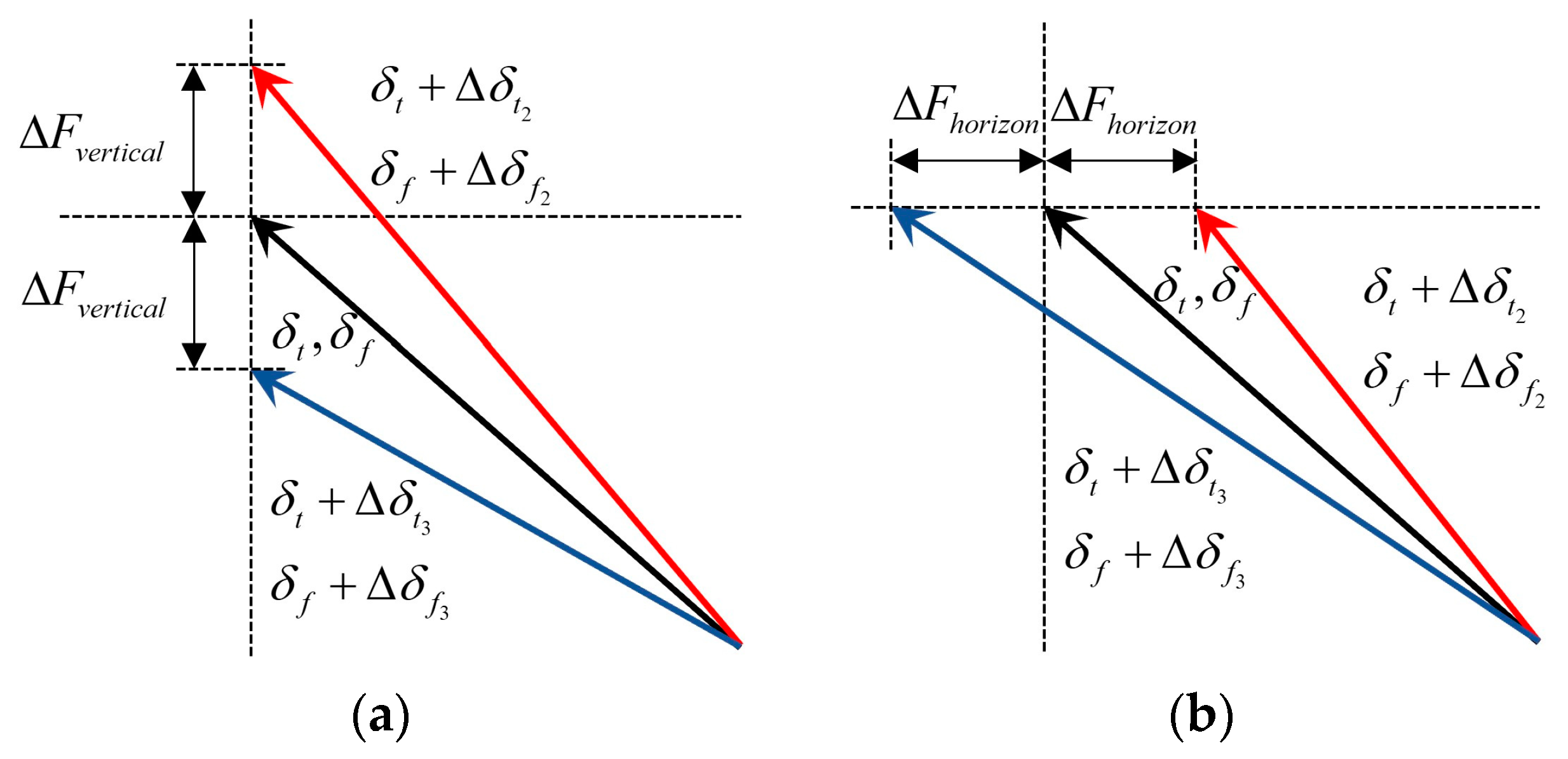
Figure 14.
Diagram of control framework.
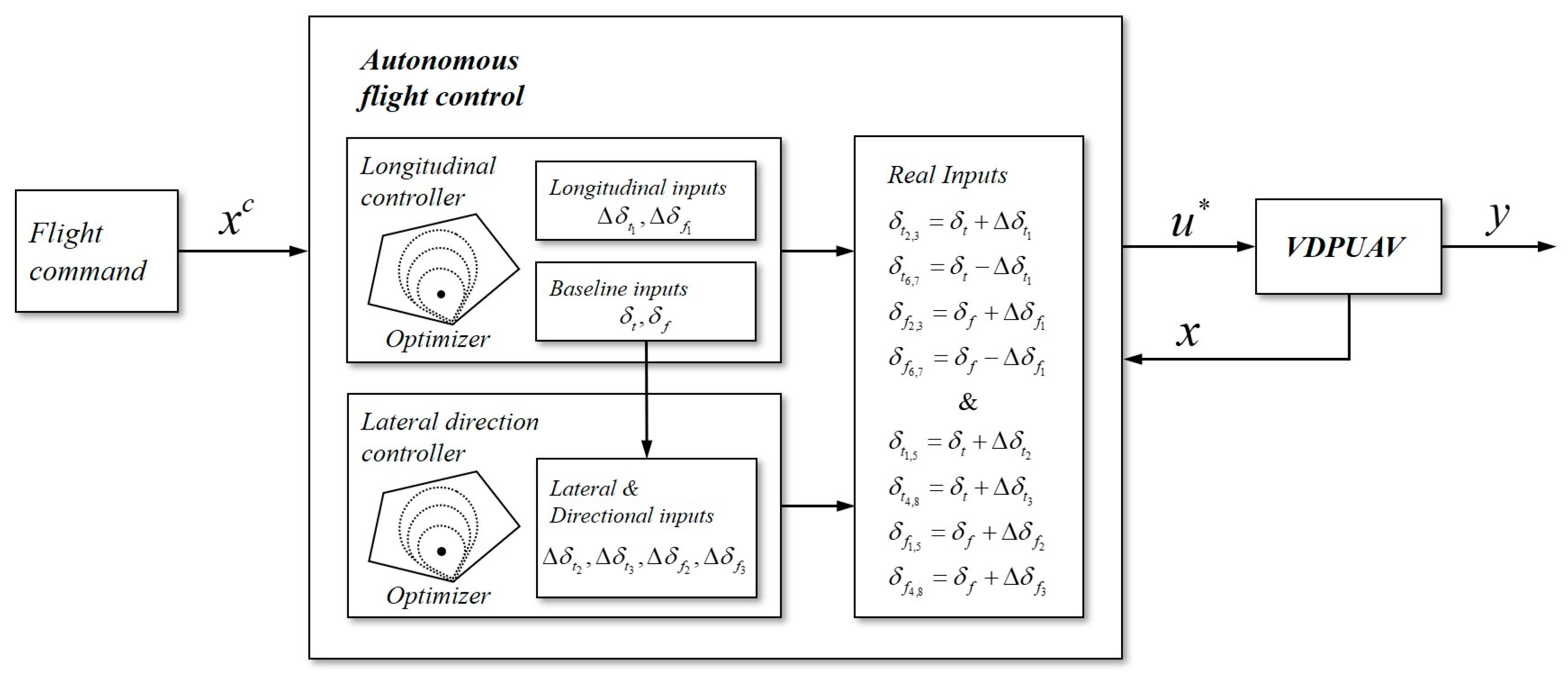
Figure 15.
Diagram of controller.

Figure 16.
Task flow of flight simulation.

Figure 17.
Response of state tracking under transition flight.
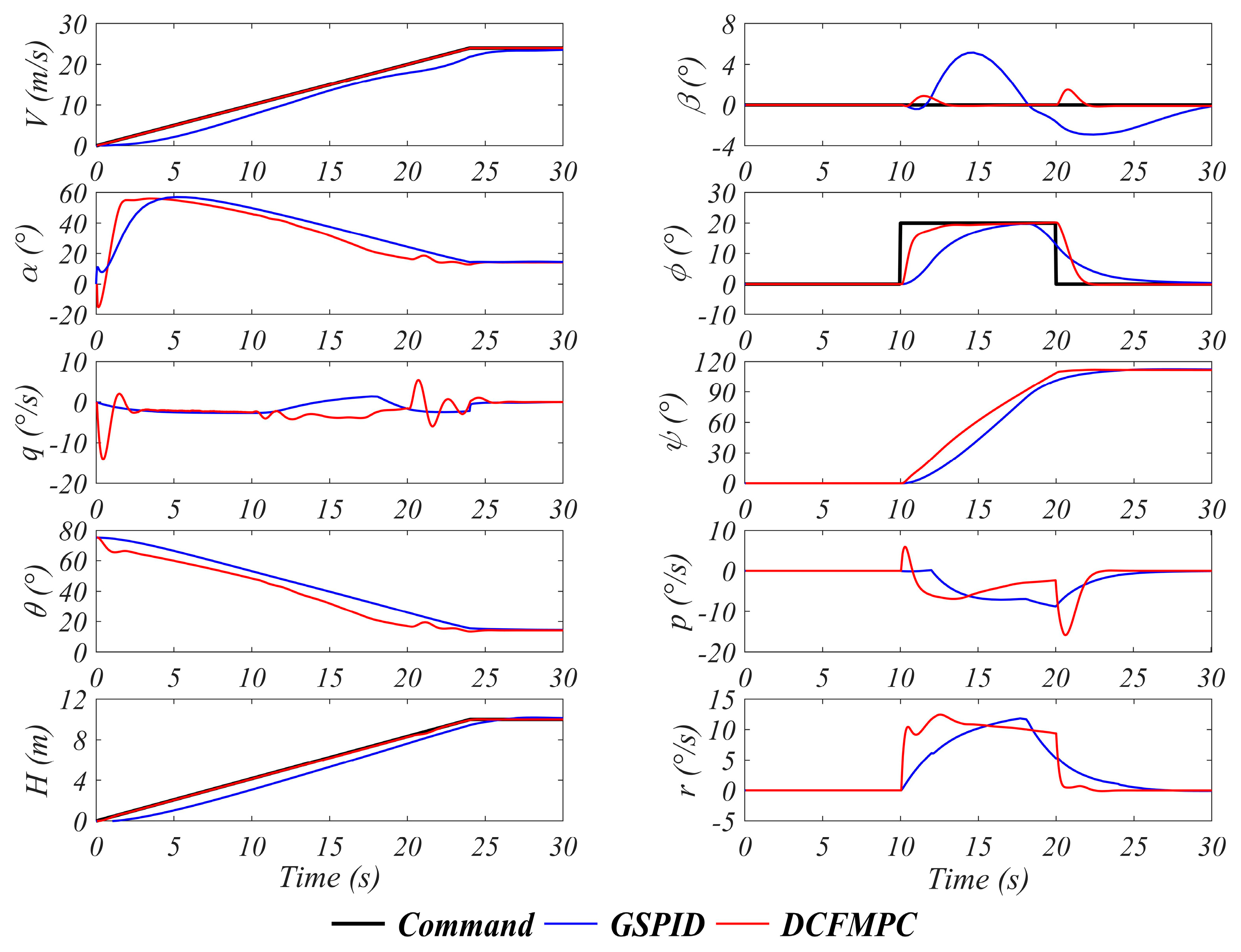
Figure 18.
Inputs response under transition flight.
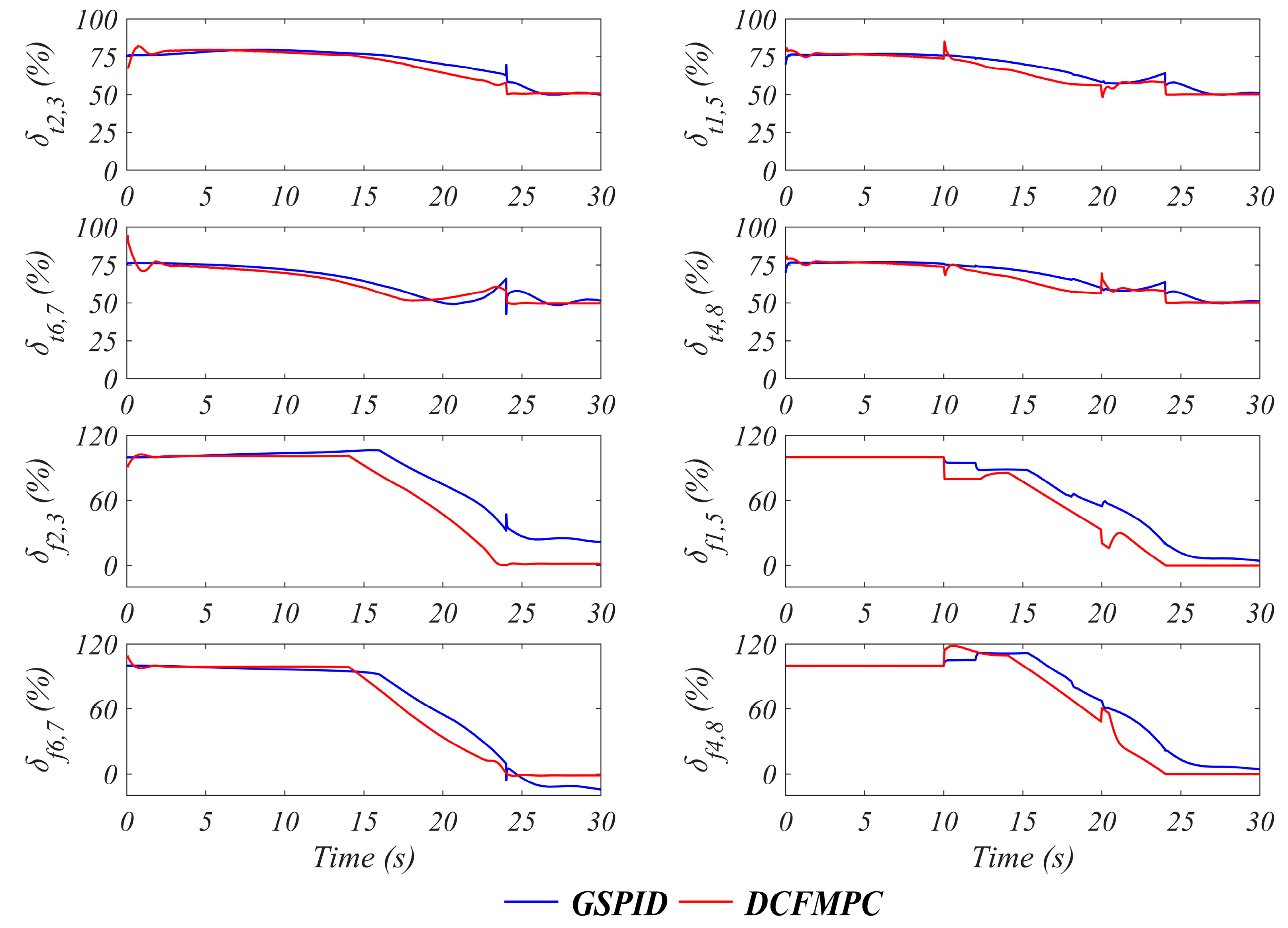
Figure 19.
Response of state tracking under cruise flight.
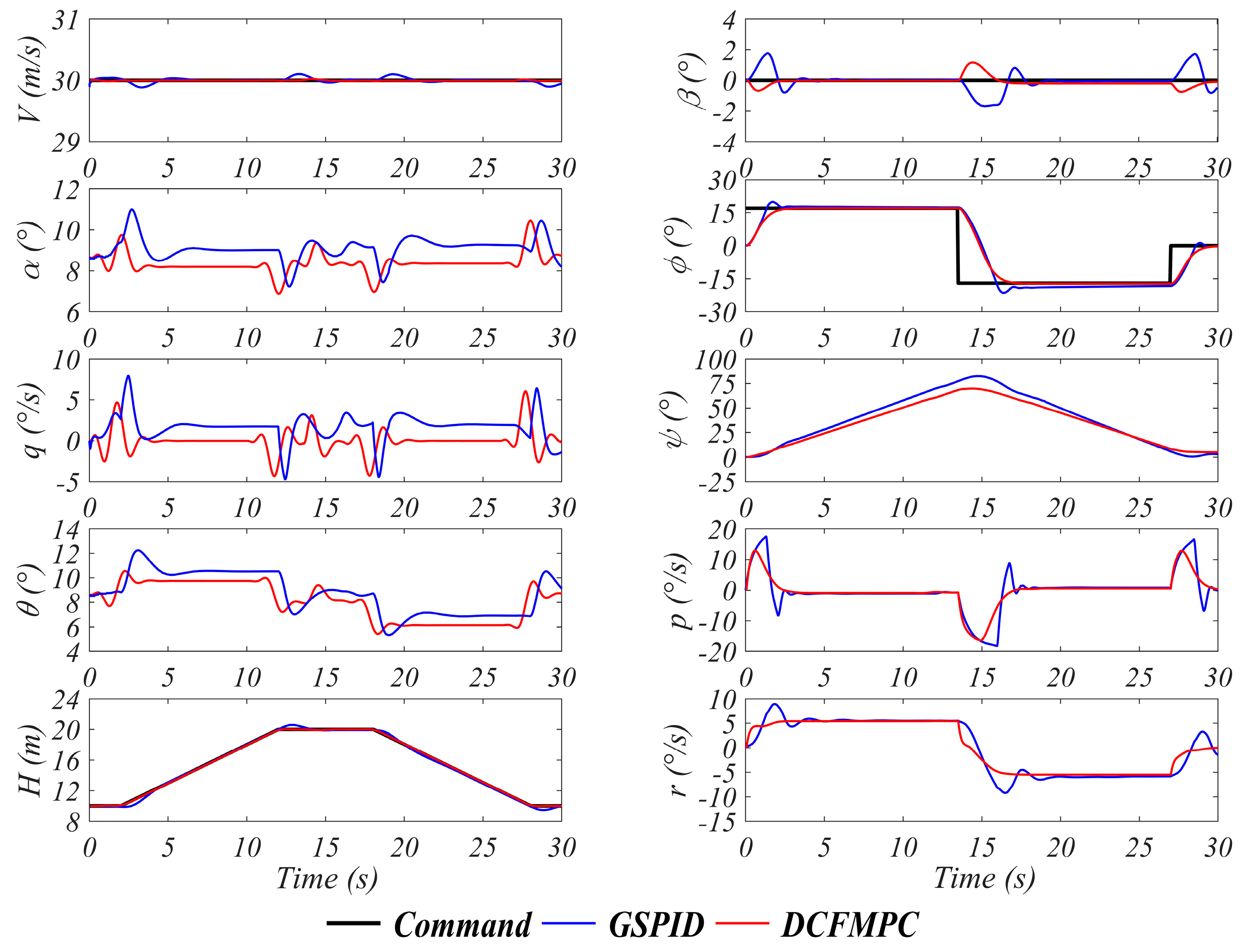
Figure 20.
Response of state tracking under maneuver flight.

Figure 21.
Response of state tracking under reverse transition flight.

Figure 22.
Inputs response under reverse transition flight.
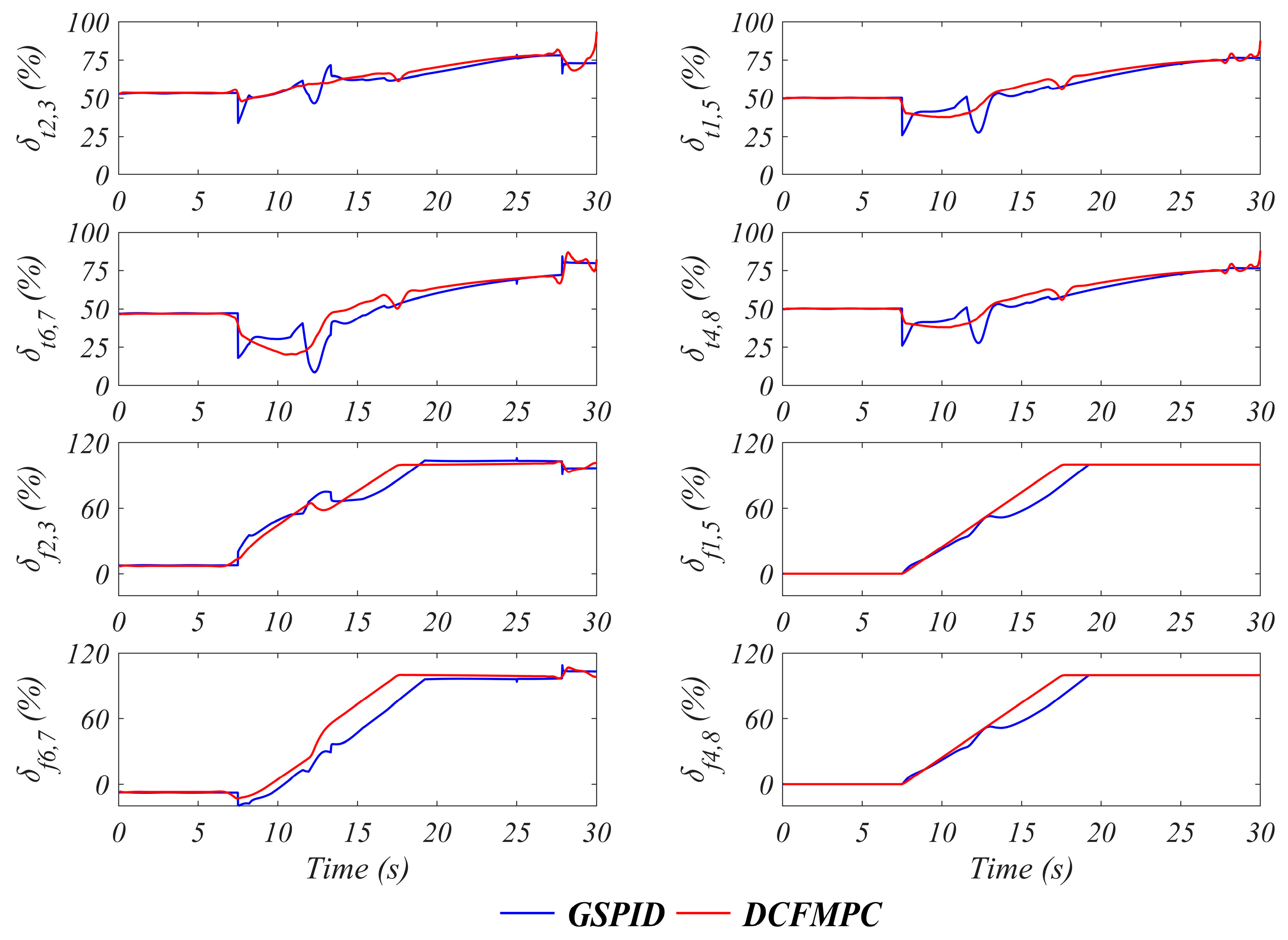
Figure 23.
Response of state tracking during cruise flight with uncertainty.
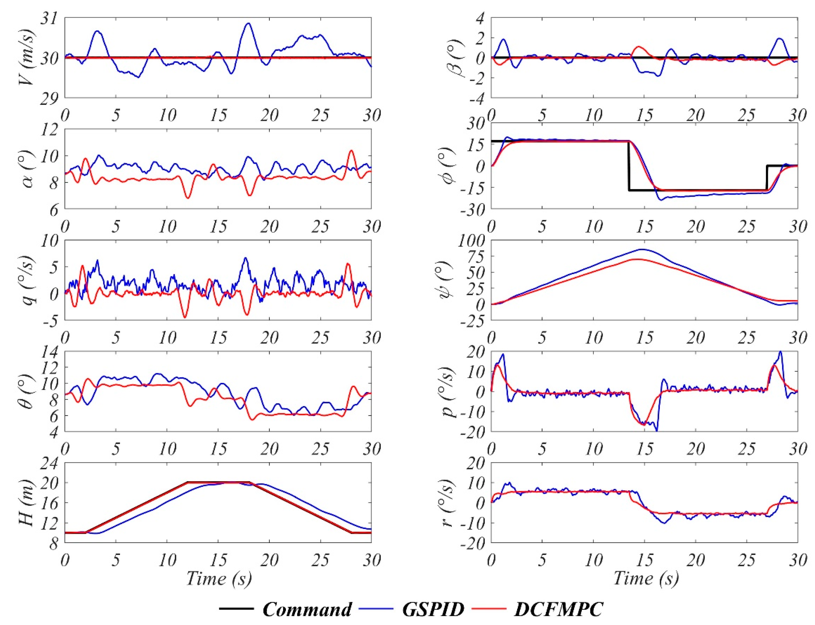
Figure 24.
Response of state tracking during reverse transition flight with uncertainty.


Table 1.
Weights for state, input and terminal costs of longitudinal controller.
| 100 | 0 | 0 | 0 | 100 | 100 | 100 | 500 | 100 | |
Table 2.
Weights for state, input and terminal costs of lateral directional controller.
| 100 | 100 | 0 | 0 | 0 | 500 | 500 | 100 | 100 | |
Disclaimer/Publisher’s Note: The statements, opinions and data contained in all publications are solely those of the individual author(s) and contributor(s) and not of MDPI and/or the editor(s). MDPI and/or the editor(s) disclaim responsibility for any injury to people or property resulting from any ideas, methods, instructions or products referred to in the content. |
© 2024 by the authors. Licensee MDPI, Basel, Switzerland. This article is an open access article distributed under the terms and conditions of the Creative Commons Attribution (CC BY) license (https://creativecommons.org/licenses/by/4.0/).
Share and Cite
MDPI and ACS Style
Xia, J.; Zhou, Z. The Modeling and Control of a Distributed-Vector-Propulsion UAV with Aero-Propulsion Coupling Effect. Aerospace 2024, 11, 284. https://doi.org/10.3390/aerospace11040284
AMA Style
Xia J, Zhou Z. The Modeling and Control of a Distributed-Vector-Propulsion UAV with Aero-Propulsion Coupling Effect. Aerospace. 2024; 11(4):284. https://doi.org/10.3390/aerospace11040284
Chicago/Turabian StyleXia, Jiyu, and Zhou Zhou. 2024. "The Modeling and Control of a Distributed-Vector-Propulsion UAV with Aero-Propulsion Coupling Effect" Aerospace 11, no. 4: 284. https://doi.org/10.3390/aerospace11040284
Note that from the first issue of 2016, this journal uses article numbers instead of page numbers. See further details here.