A Combined Experimental and Numerical Calibration Approach for Modeling the Performance of Aerospace-Grade Titanium Alloy Products

Abstract

Finite element modeling for designing and optimizing lightweight titanium aerospace components requires advanced simulation tools with adequate material modeling. In this sense, a hybrid strategy is proposed in this work to identify the parameters of the Johnson–Cook plasticity and damage laws using a combined direct-inverse method. A direct calibration method for plasticity law is applied based on the literature-reported data of strain-stress curves from experimental tensile tests at different temperatures and strain rates. The triaxiliaty-dependent fracture parameters of the Johnson–Cook damage law at reference conditions of strain rate and temperature (d₁, d₂, and d₃) are calibrated with the direct method based on new data of experimental evolution of computed average fracture strain with the average stress triaxiality. The validation is performed with numerical results from an accurate micromechanics-based Ti64 model. The inverse calibration method is used to determine the strain rate and temperature-dependent damage parameters (d₄ and d₅) through large strain simulations of uniaxial tensile tests. The numerical results, including average strain and necking profile at fracture, are then utilized to calculate stress triaxiality by the Bridgman criterion for adjusting parameters d₄ and d₅. The calibrated model yields a 2.1% error for plasticity and 3.4% for fracture predictions. The experimental and simulated load-bearing capacity using the micromechanics damage model differed by only 1%. This demonstrates that the SC11–TNT model of Ti64 is reliable for identifying the Johnson–Cook damage law through the accurate use of inverse methods. The hybrid calibration strategy demonstrates the potential capability of the identified Johnson–Cook model to accurately predict the design load-carrying capacity of Ti64 aerospace components under different deformation rates and temperatures while accounting for material damage effects.

1. Introduction

Titanium alloys are attractive engineering materials for the aerospace industry [1,2,3] mainly due to their high specific strength and ductility at low and moderate temperatures. In particular, Ti-6Al-4V (Ti64) is the most widely used titanium alloy because of its appropriate balance of processing characteristics, such as good malleability, plastic workability, heat treatability, and weldability [4]. In addition, it exhibits good biocompatibility, low density, high corrosion resistance, high compressive strength, adequate ductility, toughness, as well as the capacity to resist to impact loading and damage tolerance [4,5,6].

Finite element simulation for design of aerospace components subjected to different loadings speed requires the correct knowledge of the operational conditions, accurate boundary definitions, and adequate modeling of the investigated part material behavior. Load carrying capacity and material damage processes are strongly influenced by the speed of mechanical loads and material temperature. Extreme conditions of operating aircrafts can lead to failure in a mechanical component or structure, with potential damages including loss of human lives. Therefore, engineering calculations and analyses are conducted to predict useful life and ensure component and structural strength. Material Models—mathematical expressions representing complex physical phenomena observed in materials—are employed to forecast their loading response and deterioration.

Materials models are based on physics, generally inspired by thermodynamics and slip kinetics, and usually have a complex form [7,8,9,10,11,12]. Some frequently used Metallic Alloys Material Models are the Zirilli–Armstrong (ZA) model [13], the Bodner–Partom model (BP) [14], the mechanical threshold plasticity model (MTS) [15], the Nemat-Nasser–Guo model (NN-G) [16], and the Khan-Huang-Liang model (KHL) [17]. However, the effective prediction of the mechanical behavior of materials and design of mechanical components subjected to different strain rate and various temperatures is generally performed with the Johnson–Cook (JC) model [18]. The Johnson–Cook plasticity law is used for the design of mechanical components subjected to impact loading [6,19,20], to several strain rates and various temperatures [21], for predicting the response of a material during machining [22,23], for forming processes [24,25,26] and surface treatments [27,28]. The effects of strain hardening, strain rate sensitivity, and thermal softening are incorporated as a product for the stress response computation. Progressive material damage due to microstructural changes such as nucleation, cavity growth, coalescence, and propagation of microcracks is incorporated in the model through several damage parameters dependent on stress triaxiality, strain, temperature, and strain rate. Due to its simplicity, Johnson–Cook is one of the most widely used models [10,22,25,29,30]; however, some studies limit its application. For instance, Tuninetti et al. [31] showed that this model is only suitable for predicting the plastic deformation behavior of Ti64 with temperatures below 400 °C.

Understanding the limitations and possible modifications of the Johnson–Cook model for titanium alloys is critical to optimizing the design and manufacturing processes of aerospace components. Modifications to the original Johnson–Cook model have been proposed to improve predictions [32,33,34,35,36,37], however, implementing and adapting them in finite element software is not straightforward. The modifications are justified by unique microstructural properties observed in the investigated alloys, demonstrating improved prediction accuracy of mechanical responses to different loading conditions [38].

One of the most widely accepted criticisms of the Johnson–Cook model is that it oversimplifies material behavior by assuming isotropic hardening [39,40,41]. In addition, some studies have shown that the damage parameter in the Johnson–Cook model may not fully represent the complexity of material damage, especially in cases where multiple damage mechanisms occur [36,42]. Furthermore, model modifications to the constitutive equation for titanium alloys may introduce additional complexity, particularly for software implementation and calibration, without significantly improving the accuracy of the model predictions. Finally, the required accuracy of results for a specific application or design requirements is the most important criterion for determining the limitations of the Johnson–Cook model, since, for certain studies, this model may not adequately capture the material behavior, while whereas, for other studies, similar results may be considered acceptable.

The Ti64 models based on Johnson–Cook equations differ in the strategy used for parameter calibration. The model parameters can be obtained through experimental results using a direct identification method [43,44,45] or inverse analysis [46,47,48,49,50]. The differences between the results obtained with these methods depend mainly on the quality of the simulations, observed variables, and applied models to determine virtual or simulation parameters. Therefore, this study focuses on the accuracy of calibration methods for JC model plasticity and damage-related parameters required for aerospace engineering design of Ti64 components. First, the direct identification method is applied for the plasticity parameters and the damage-related parameters affecting the material behavior at the reference temperature and strain rate conditions. Subsequently, damage parameters associated with the combined effect of temperature and strain rate are calibrated using finite element inverse simulations with an accurate micromechanics-based damage model from the literature. The main originality of this work is the proposal of a hybrid calibration strategy of the Johnson–Cook model when some missing data from experiments are a constraint. In addition, the calibrated set of Johnson–Cook parameters for the Ti64 alloy that includes all the capabilities of the model in plasticity and damage is highlighted as the main contribution for applications to aerospace engineering design, aeronautical structures, and in general, manufacturing optimization and critical mechanical components under operation of Ti64 titanium alloy parts.

2. Materials and Methods

2.1. Characteristic Properties of the Investigated Ti64 Titanium Alloy

The microstructure of the Ti64 alloy consists of primary α -grains, hexagonally packed compactly packed (hcp) embedded in a two-phase matrix (Figure 1). The matrix is composed of alternating lamellae of a primary α -phase and a body-centered cubic β -phase. This alloy exhibits anisotropic behavior in different directions of the material characterized by Young’s modulus, initial flow stress, and strain hardening [51].

The average grain size is of equivalent ellipsoidal shape with a length and width of 12 ± 3 and 6 ± 2 μm, respectively, measured according to the linear intersection method on micrographs taken with a field emission scanning electron microscope (FESEM). The elemental composition determined directly by energy-dispersive X-ray spectroscopy (EDS) is shown in

Table 1. Chemical composition of Ti64 alloy.

Al	V	Fe	N	O	C	Ti
6.1	4.0	0.3	0.05	0.2	0.08	Balance

, equivalent to a Grade 5 alloy by ASTM B265 standard.

Split Hopkinson bar experiments are frequently used to characterize the high strain rate mechanical behavior of metals. These experiments yield the specimen’s strength and elongation history, reflecting its material and structural behavior. Calculating the actual material behavior from this global response is not simple; certainly, for materials such as Ti64, due to the low strain hardening, the sample deformation is very heterogeneous. However, for fundamental materials research and modeling of constitutive materials, knowledge of the true effective stress versus plastic strain, strain rate, and temperature is essential [52]. The mechanical properties for tensile strength of Ti64 alloy are shown in

Table 2. Summary of mechanical properties determined directly from the quasi-static true tensile strain-stress curve at room temperature [4].

$\mathbf{Strain} \mathbf{Rate}, \dot{\mathit{\epsilon }}$  ${(\mathbf{s}}^{-1})$	Young’s Modulus, E (GPa)	$\mathbf{Initial} \mathbf{Yield} \mathbf{Stress}, {\mathit{\sigma }}_{0.2\mathit{\%}}$ (MPa)	$\mathbf{True} \mathbf{Fracture} \mathbf{Strain}, {\mathit{\epsilon }}_{\mathit{f}}$	True Stress at Fracture (MPa)
0.001	111 ± 1	927 ± 3	0.41	1241

.

The experimental procedures, including the specific testing conditions and equipment used for the tensile tests at different temperatures and strain rates are previously reported in different studies. Lecarme et al. [53] performed tensile test in miniaturized tensile samples of 3 mm diameter at strain rates of ${10}^{-5}{ \mathrm{s}}^{-1}$, ${7.6 \mathrm{s}}^{-1}$, ${2 \mathrm{s}}^{-1}$, and temperature of 25 °C. Tuninetti et al. [54] performed tensile tests in 6 mm diameter cylindrical samples aided with digital image correlation applied in image recorded from stereo-cameras for computing the evolving deformed shape of samples using Vic3D software. The strain rates applied were $7.5\times {10}^{-5} {\mathrm{s}}^{-1}$, ${10}^{-3}{ \mathrm{s}}^{-1}$, ${10}^{-2}{ \mathrm{s}}^{-1}$, and ${10}^{-1} {\mathrm{s}}^{-1}$ at 25 °C, and for high temperature testing, 150 °C and 400 °C were selected at ${10}^{-3}{ \mathrm{s}}^{-1}$. For high strain rate testing at ${1150 \mathrm{s}}^{-1}$, Peirs et al. [55] used the Split Hopkinson bar equipment at University of Ghent. The dogbone samples of 2.5 mm diameters were used and the high speed digital image correlation allowed to obtain local strain data.

2.2. Johnson–Cook Constitutive Model of Plasticity and Damage

The plasticity and damage model proposed by Johnson–Cook is an empirical constitutive model that arises from the need to calculate intense impulsive charging due to high-velocity impacts and explosive detonations. Unlike other models, this model includes strain rate dependence for both deformation and failure of the material [18,29].

2.2.1. Strain Hardening, Strain Rate Strengthening, and Temperature Softening

The Johnson–Cook plasticity model [18] describes the equivalent von Mises stress ($\overline{\sigma }$) (Equation (1)) dependent on the equivalent plastic strain ($\epsilon$), the equivalent plastic strain rate ($\dot{\epsilon }$) and temperature ($T$).

$$\overline{\sigma }=\left(A+B{\epsilon }^n\right)\left[1+C·ln\left(\frac{\dot{\epsilon }}{\dot{{\epsilon }_0}}\right)\right]\left(1-{T^{*}}^m\right)$$

(1)

The term $A$ corresponds to the yield stress at a reference temperature $\left(T_0\right)$ and reference strain rate ($\dot{{\epsilon }_0}$). Coefficient $B$ and strain hardening exponent $n$ describe the reference strain-stress curve, while $C$ identifies the sensitivity of the material to the strain rate. Finally, the effect of hardening with temperature, is described with the homologous temperature ($T^{*}$) and thermal softening ($m$). The temperature of the deformation process based on homologous temperature is defined as a fraction of the melting point (Equation (2)).

$$T^{*}=\left(T-T_0\right)/\left(T_{melt}-T_0\right)$$

(2)

$T_0$ is the reference temperature set at 25 °C, and $T_{melt}$ is the melting temperature of the material [56,57,58].

2.2.2. Damage and Failure Criteria

The Johnson–Cook damage model given in Equation (3) describes the fracture strain $\left({\epsilon }_f\right)$ as a function of stress triaxiality ($\eta$), strain rate, and temperature. The Johnson–Cook fracture model expression comprises three factors. The first term indicates that fracture strain decreases with increasing hydrostatic stress $\left(p\right)$, and the second and third terms relate the change in material ductility to strain rate and thermal softening, respectively.

$${\epsilon }_f=\left[d_1+d_2{e}^{{-d}_3\eta }\right]·\left[1+d_4\mathrm{l}\mathrm{n}\left(\frac{\dot{\epsilon }}{\dot{{\epsilon }_0}}\right)\right]·\left(1+d_5{T}^{*}\right)$$

(3)

The parameters $d_i$ with $i=1, 2,\dots , 5$ are the damage-related material constants, $\dot{{\epsilon }_0}$ is the reference strain rate, and $\eta$ is the stress triaxiality defined as the ratio of the hydrostatic pressure $\left(p\right)$ over the equivalent von Mises stress $\overline{\sigma }$[29,59]. According to this law, fracture occurs when the damage index $D$ increases with the cumulative plastic strain until the value 1 is reached (Equation (4)) [59].

$$D=\int \frac{d\epsilon }{{\epsilon }_f}$$

(4)

3. Hybrid Calibration Method

In this work, the direct calibration strategy is based on two techniques: (a) a linear regression method and (b) the generalized reduced gradient technique. For the non nonlinear optimization, the analytical model JC prediction is compared with post-processed experimental data minimizing the error with an objective function such as Equation (5) [46,60,61]. Inverse identification is based on minimizing the normalized error (Equation (5)) between the finite element predictions of the model and the experimental measurements using the Levenberg–Marquardt approach [62]. The general objective function for error is shown in Equation (5), which normalized the data and avoid weighting of higher values. The normalized error between stress from test results ($\sigma \_exp$) and analytical model or numerical simulation ($\sigma \_model$) can be computed for each pair of data, such as strain or displacement (i) for the total number of sampling considered (n) and the total number of data curves ($n_m$). The average error value is finally obtained by dividing the total amount of data curves considered ($n_m$). MAPE stands for mean average percentage error. Accurate fit is defining for values lower than 5% as assumed for this type of material and models.

$$\mathrm{M}\mathrm{A}\mathrm{P}\mathrm{E}=\frac{1}{n_m}\sum _{m=1}^{n_m}{\sum }_{i=1}^n\frac{\left|{\sigma \_exp}_i-{\sigma \_model}_i\right|}{{\sigma \_exp}_i}\times 100$$

(5)

3.1. Identification of Johnson-Cook Plasticity Constants

The direct calibration method was applied to determine the parameters of the Johnson–Cook (JC) plasticity model (Equation (1)). The normalized error between stress data computed from experiments and analytical JC plasticity model was globally minimized for tensile tests at 25 °C, 150 °C, and 400 °C, and at different strain rates of ${1150 \mathrm{s}}^{-1}$, ${7.6 \mathrm{s}}^{-1}$, ${2 \mathrm{s}}^{-1}$, ${10}^{-3}{ \mathrm{s}}^{-1}$, ${10}^{-2}{\mathrm{s}}^{-1}$, ${10}^{-1} {\mathrm{s}}^{-1}$, and $7.5\times {10}^{-5} {\mathrm{s}}^{-1}$. Each stress strain data curve at specific temperature and strain rate used for the identification was the average data from three tests.

Note that uniaxial tensile strain data were previously determined by different authors. For strain rate tests at ${10}^{-5}{ \mathrm{s}}^{-1}$, ${7.6 \mathrm{s}}^{-1}$, ${2 \mathrm{s}}^{-1}$, Lecarme et al. [53] used miniaturized tensile samples of 3 mm diameter at the Catholic University of Leuven. The tests data from strain rate of $7.5\times {10}^{-5} {\mathrm{s}}^{-1}$, ${10}^{-3}{ \mathrm{s}}^{-1}$, ${10}^{-2}{ \mathrm{s}}^{-1}$, and ${10}^{-1} {\mathrm{s}}^{-1}$, including the thermal curves performed at the University of Liège were obtained from Tuninetti et al. [54] (Figure 2). The highest strain rate curves of ${1150 \mathrm{s}}^{-1}$ have been obtained from tests performed at the University of Ghent [55] with the Split Hopkinson bar technique.

For the identification, first the reference temperature of 25 °C and the reference strain rate of ${10}^{-3}{\mathrm{s}}^{-1}$ are considered. Model parameter $A$ is determined as the yield stress under the given reference conditions. To calculate parameters $B$ and $n$, the test temperature ($T$) is equated with the reference temperature ($T_{ref}$) and the test strain rate ($\dot{\epsilon }$) with the reference strain rate (${\dot{\epsilon }}_{ref}$), eliminating the factors of Equation (1) dependent on these variables to obtain Equation (6).

$$\overline{\sigma }=\left(A+B{\epsilon }^n\right)$$

(6)

Rearranging the obtained equation and applying natural logarithm to both sides of the equation, the linear relationship between both sides of Equation (7) is plotted obtaining a linear fitting. From the slope and the intersection of the this fitted line, the constants $B$ and $n$ are identified.

$$\ln \left(\overline{\sigma }-A\right)=n\ln \epsilon +\ln B$$

(7)

The parameter $C$ is subsequently obtained by equating the test temperature ($T$) with $T_{ref}$, reducing the equation as only strain rate-dependent (Equation (8)).

$$\frac{\overline{\sigma }}{\left(A+B{\epsilon }^n\right)}=\left[1+C·ln\dot{{\epsilon }^{*}}\right]$$

(8)

The computed values of A, B, and n are replaced in Equation (8), and the data from the tests with different strain rates at room temperature are plotted on the orthogonal axes $\frac{\overline{\sigma }}{\left(A+B{\epsilon }^n\right)}$ and $ln\dot{{\epsilon }^{*}}$, obtaining a linear fit which determines the value of the constant C from the slope of the curve.

The parameter $m$ is determined by using data at the test strain rate ($\dot{\epsilon }$) of the reference (${\dot{\epsilon }}_{ref})$, eliminating the strain rate dependent factor. Equation (1) is rearranged, leaving the temperature-dependent part on one side of the equation, and by applying natural logarithm, the following form is obtained (Equation (9)).

$$\mathrm{Ln}\left[1-\frac{\overline{\sigma }}{\left(A+B{\epsilon }^n\right)}\right]=m\ln T^{*}$$

(9)

By replacing the values of the material constants $A$, $B$, and $n$ in Equation (9) and obtaining the trend line of the data at temperatures 150 °C and 400 °C, the constant $m$ is determined.

3.2. Calibration of Johnson-Cook Damage Parameters

To determine the model parameters of the Johnson–Cook damage law (Equation (3)), the direct method is applied for the parameters $d_1$, $d_2$, and $d_3$. The inverse analysis from finite element simulations is selected to calibrate a micromechanical-based damage model adapted to compute the force-displacement curves and sample deformed shape at fracture under different strain rates and temperatures. The numerical process data are used to obtain stress triaxiality and fracture for the calibration of damage parameters $d_4$ and $d_5$.

3.2.1. Direct Calibration of Damage Parameters at Reference Condition ($d_1$, $d_2$, and $d_3)$

To determine the parameters $d_1$, $d_2$, and $d_3$, fractured specimens geometry deformed at reference temperature and reference strain rate are required to reduce the Johnson–Cook (JC) damage model (Equation (3)) to Equation (10).

$${\epsilon }_f=\left[d_1+d_2{e}^{-d_3\eta }\right]$$

(10)

The stress triaxiality can be computed using the Bridgman analytical model given in Equation (11) [63].

$$\eta =\frac{1}{3}+\mathrm{l}\mathrm{n}\left(1+\frac{a}{2 R}\right)$$

(11)

$R$ and $a$ are values obtained experimentally just before fracture, corresponding to the circumferential notch radius and the minimum cross-sectional radius, respectively. This minimum cross-sectional radius at fracture and the initial cross-section of the samples allow computing the fracture strain with the classical true strain definition.

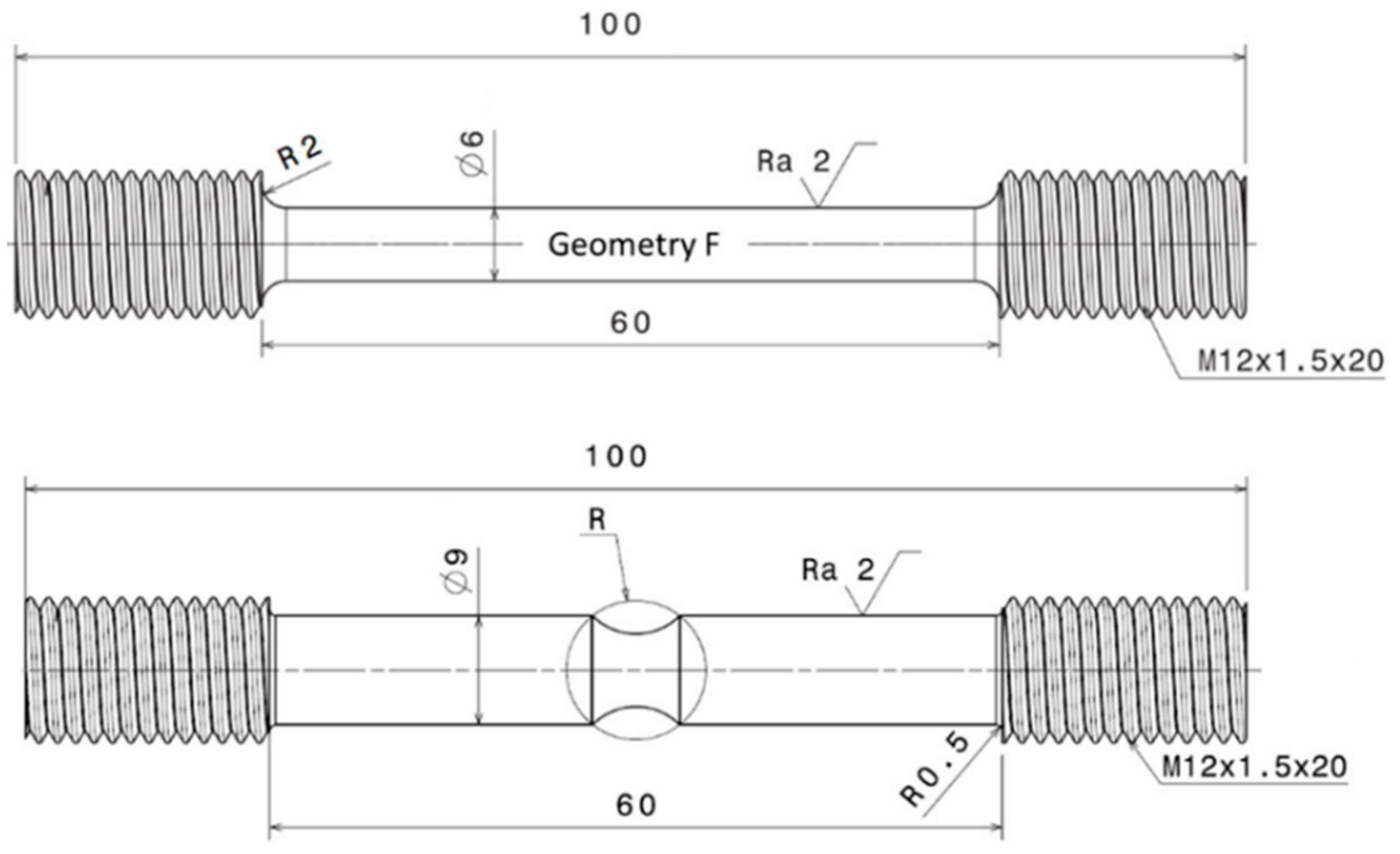
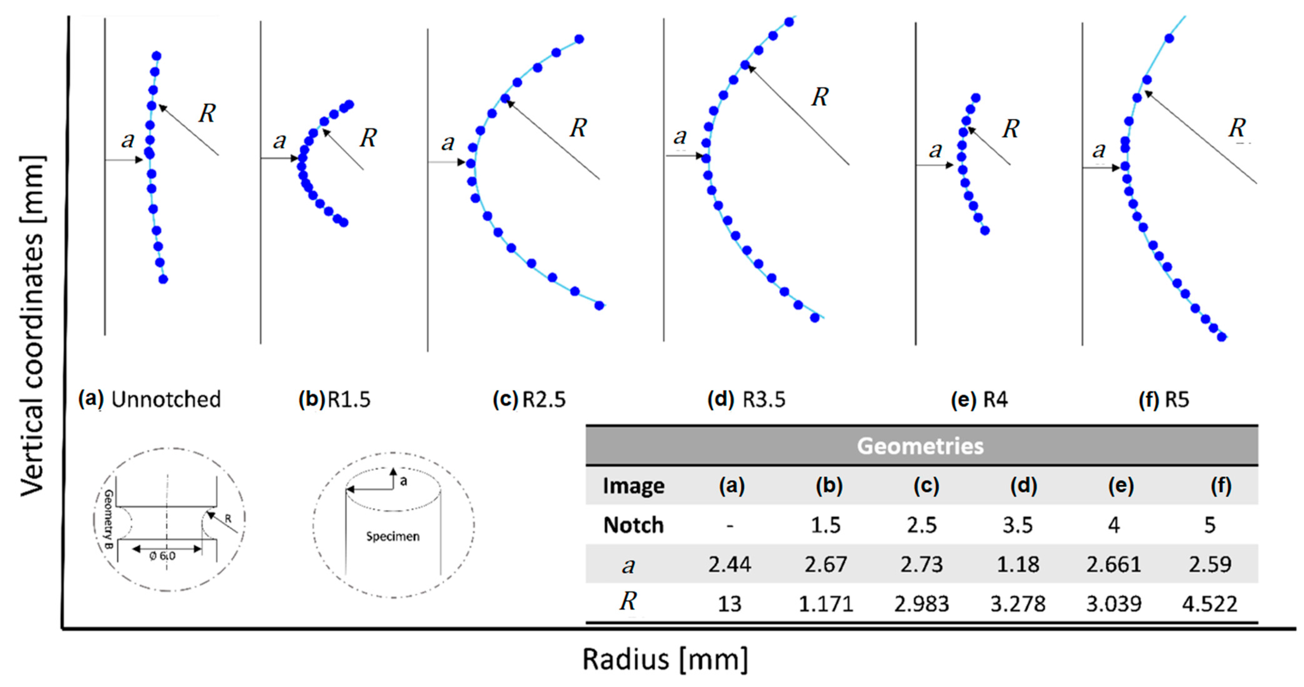
In the reference condition, the model constants of analytical JC damage are computed by minimizing the objective function such as Equation (5) with the non nonlinear optimization technique of generalized reduced gradient explained at the first paragraph of Section 3. In this case, the objective function to minimize is dependent on the fracture strain for certain values of triaxiality, instead of stress and strain variables defined in Equation (5). To obtain a large set of experimental data points of fracture strain vs. 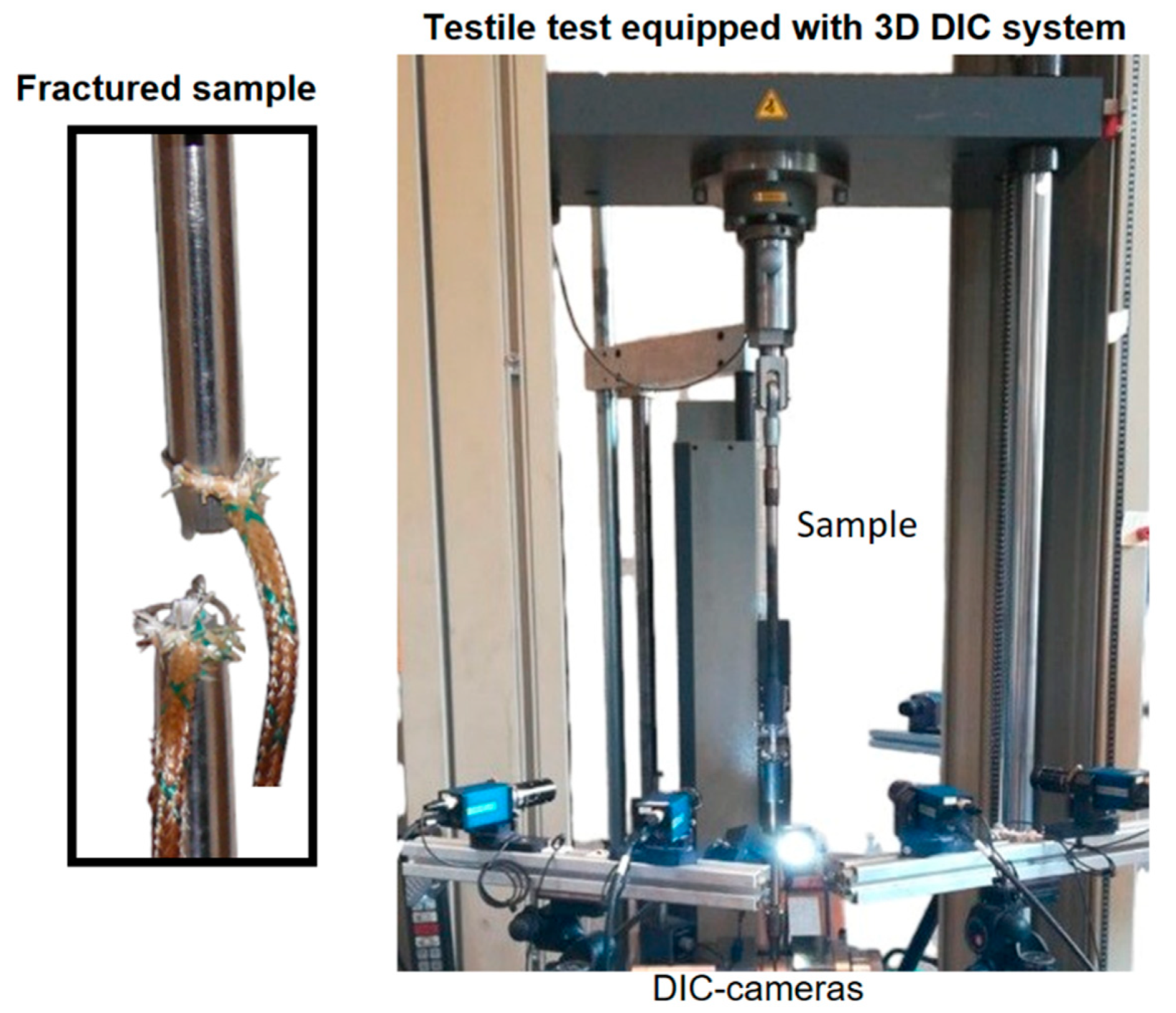stress triaxiality, a total of six type of cylindrical specimens of the alloy with different geometries were analyzed (Figure 3): cylindrical with no initial notch, and notched cylinders with radii of R1.5, R2.5, R3.5, R4, and R5. The three tested samples of each geometry were measured until rupture with using stereovision CCD devices and analyzed with digital image correlation, providing accurate notch shape evolution measurements with a maximum error of about 2 $\mathsf{\mu }\mathrm{m}$, as reported in previous research [51].

The stereoscopic camera setup allows representation of each object point on a specific pixel on the image plane of each camera. By utilizing the imaging parameters and orientations of the cameras, such as intrinsic parameters (focal length, principle point, and distortion parameters) and extrinsic parameters (rotation matrix and translation vector), the position of each object point can be calculated in 3D. The analysis was performed using Commercial Vic3D DIC software from Correlated Solutions Inc., Columbia, SC, USA, along with Limess system from Limess Messtechnik und Software GmbH, Pforzheim, Germany. The following steps were required for the accurate measurements in terms of adequate surface reconstruction of the sample in the three-dimension space. Optimal size for spray paint ranged from 3 × 3 to 10 × 10 pixels. Cables and camera supports were fixed for eliminating any vibrations or relative movement that could affect cameras calibration. Lamps at various positions were tried to achieve suitable lighting without creating reflections in the image and light isolating the testing environment to maintain consistent brightness. Experimental resolution improvements of CCD cameras were achieved with 50 mm lenses along with extension tubes of 10 mm. The resulting image resolution of 30 µm/pixel provided the required shape accuracy. For obtaining sharp images, adjustment was performed until optimal values of f/5.6 for aperture, 15 ms for exposure time, and a depth-of-field focus range of 5–10 mm was reached.

3.2.2. Inverse Identification of the Damage Parameters $d_4$ and $d_5$

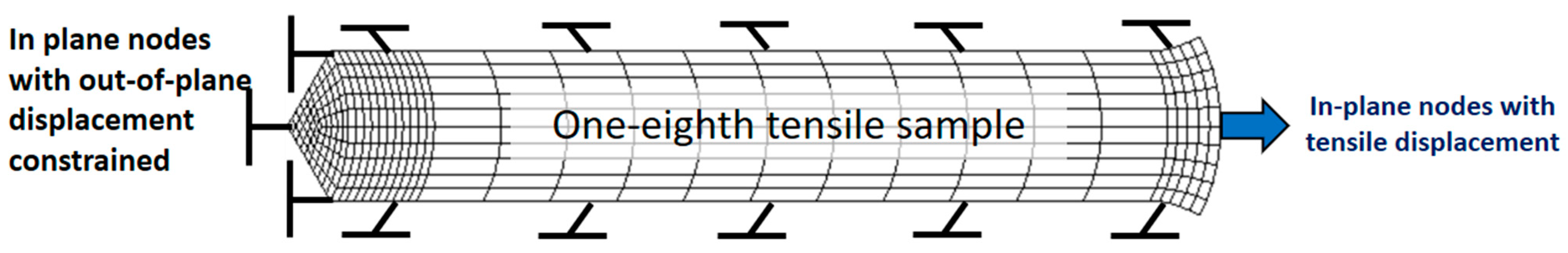
The simulated test conditions performed with the finite element LAGAMINE software are shown in

Table 3. Test condition simulations for the inverse identification of damage constants $d_4$ and $d_5$.

Simulations	$\mathbf{Temperature} \left(\mathit{T}\right)$	$\mathbf{Strain} \mathbf{Rate} \left(\dot{\mathit{\epsilon }}\right)$
Simulation 1	Room temperature	${10}^{-2}{ \mathrm{s}}^{-1}$
Simulation 2	Room temperature	${10}^{-4}{ \mathrm{s}}^{-1}$
Simulation 3	150 °C	${10}^{-3}{ \mathrm{s}}^{-1}$
Simulation 4	400 °C	${10}^{-3}{ \mathrm{s}}^{-1}$

. The mesh of the simulated samples shown in Figure 4 is performed with 2025 eight-node hexahedral BWD3D elements based on the nonlinear three-field Hu–Washizu variational principle of stress, strain and displacement [64,65,66]. A refinement zone was set in the middle of the sample where localization necking and higher stress–strain gradients appears previous to fracture. The samples are displacement controlled in the thread zone with a ramp displacement reaching maximum values between 3 and 4 mm depending on the simulated condition of strain rate and temperature (see details in Results Section 4.3, for maximum displacement). Note the symmetry condition in three orthogonal planes is selected and only one eight of the sample is modeled. The mechanical law of the material used for these simulations was the Cazacu law (Equation (12)), which is integrated into the software and incorporates the CPB06 yield criterion and Voce’s strain hardening law [51,67,68]. In addition, the SC11–TNT damage model [39], an extension of CPB06 plasticity is used for local state values computations such as stress triaxiality based on micromechanics failure. As a cutting plane algorithm in a semi-implicit method was used for the implementation, the convergence at the global level of the finite element routine is linked to the global time step size. The computational efficiency, stability, and robustness of the law was obtained with the verified convergence criterion and time step size to avoid convergence problems. More details regarding the implementation of the model and simulation parameters can be found in Rojas-Ulloa et al. [69]. The Cazacu-plasticity related parameters are given in

Table 4. CPB06 model constants (Cij) for Ti64 reported in [51].

Plastic Work Per Volume (W/m3)	CPB06 Model Constants
	C11	C12	C13	C22	C23	C33	C44 = C55 = C66
1.86	1	−2.37	−2.36	−1.84	1.20	−2.44	−3.61
9.38	1	−2.50	−2.93	−2.28	1.28	−2.45	4.02
48.6	1	−2.43	−2.92	1.65	−2.24	1.00	−4.00
100	1	−2.57	−2.88	1.39	−2.38	0.88	−3.93
207	1	−2.97	−2.93	0.53	−2.96	0.44	−3.88

. The hardening/softening law was adapted to describe the experimentally obtained force versus displacement data at each tests condition for the total displacement test until rupture. The final obtained geometry of the fractured samples was further analyzed for the computation of the damage parameters as explained hereafter.

The CPB06 equivalent stress for the studied Ti64 is given in Equation (12).

$${\overline{\sigma }}^{\mathrm{CPB}06}={\tilde{m}\left\{{\left(\left|{\sum }_1\right|-k{\sum }_1\right)}^2+{\left(\left|{\sum }_2\right|-k{\sum }_2\right)}^2+{\left(\left|{\sum }_3\right|-k{\sum }_3\right)}^2\right\}}^{\frac{1}{2}}$$

(12)

${\sum }_1$, ${\sum }_2$, ${\sum }_3$ are the principal values of the tensor $\sum =\mathrm{C}:\mathrm{S}$, where C is the orthotropy tensor and S is the deviator of the Cauchy tensor. C_ij are the CPB06 model constant for the Ti64 [70]. The material constant $\tilde{m}$ describes the equivalent stress hardening in the tensile direction, which is based on the Voce hardening law (Equation (13)):

$$\sigma \left({\overline{\epsilon }}_p\right)=A+B\left[1-\exp \left(-C{\overline{\epsilon }}_p\right)\right]$$

(13)

A, B, and C are the hardening constants for specific strain rate and temperature of the material, which are identified by inverse calibration until the simulated load displacement curve reached the experimental curve.

Note that for the simulated tests conditions, even if the test range for the calibration of the parameter $d_4$ is between the quasi-dynamic and the very low strain rate, the exponential order difference in two digits covers the significant range of half of the total strain rate regime between ${10}^{-3} {\mathrm{s}}^{-1}$ and ${10}^3 {\mathrm{s}}^{-1}$. This sensitivity of fracture is similar in the full strain rate regime as given by the Johnson–Cook damage criteria (Equation (3)).

The fracture features of the simulated samples, computed with the constants of the Voce stress–strain law varied until accurate prediction of the experimental force-displacement data of each simulated case was achieved, allowing us to obtain the stress triaxiality with the Bridgman method for each simulated specimen. In addition, the state variables given by the Cazacu plasticity law (CPB06) allows to obtain the local value without damage. To calculate the damage parameter $d_4$, the results of the simulations at room temperature and two different strain rates are used to eliminate the temperature-dependent component of the damage criteria (Equation (3)). This allows to obtain Equation (14).

$${\epsilon }_f=\left[d_1+d_2{e}^{{-d}_3\eta }\right]·\left[1+d_4\mathrm{l}\mathrm{n}\left(\frac{\dot{\epsilon }}{\dot{{\epsilon }_0}}\right)\right]$$

(14)

Equation (14) is properly rearranged for applying the linear regression method, leaving the strain rate-dependent part on one side and applying a natural logarithm on both sides (Equation (15)).

$$\frac{{\epsilon }_f}{\left[d_1+d_2{e}^{-d_3\eta }\right]}-1=d_4\mathrm{l}\mathrm{n}\left(\frac{\dot{\epsilon }}{\dot{{\epsilon }_0}}\right)$$

(15)

The values of the constants $d_1$, $d_2$, and $d_3$ already obtained are replaced, and the data from the simulations with different strain rates at room temperature are plotted on the axes $\frac{{\epsilon }_f}{\left[d_1+d_2{e}^{{-d}_3\eta }\right]}-1$ and $\mathrm{l}\mathrm{n}\left(\frac{\dot{\epsilon }}{\dot{{\epsilon }_0}}\right)$. This provides the linear trend with the corresponding slope the value of the constant $d_4$.

The parameter $d_5$ is calculated with the results of the simulations of test at reference strain rate and temperatures different from the reference. This eliminates the strain rate-dependent component from the damage criterion (Equation (16)).

$${\epsilon }_f=\left[d_1+d_2{e}^{-d_3\eta }\right]·\left(1+d_5{T}^{*}\right)$$

(16)

The equation is rearranged, leaving the strain rate-dependent part on one side of the equation, using the natural logarithm of the equation, represented in Equation (17).

$$\frac{{\epsilon }_f}{\left[d_1+d_2{e}^{{-d}_3\eta }\right]}-1=d_5{T}^{*}$$

(17)

The values of the constants $d_1$, $d_2$, and $d_3$ obtained are replaced, and the data from the simulations obtained for different temperatures at the reference strain rate are plotted on the horizontal axis $\frac{{\epsilon }_f}{\left[d_1+d_2{e}^{-d_3\eta }\right]}-1$ and the vertical axis $T^{*}$. Finally, by the linear fitting, the slope determines the value of the constant $d_5$.

4. Results and Discussion

4.1. Plasticity-Related Parameters

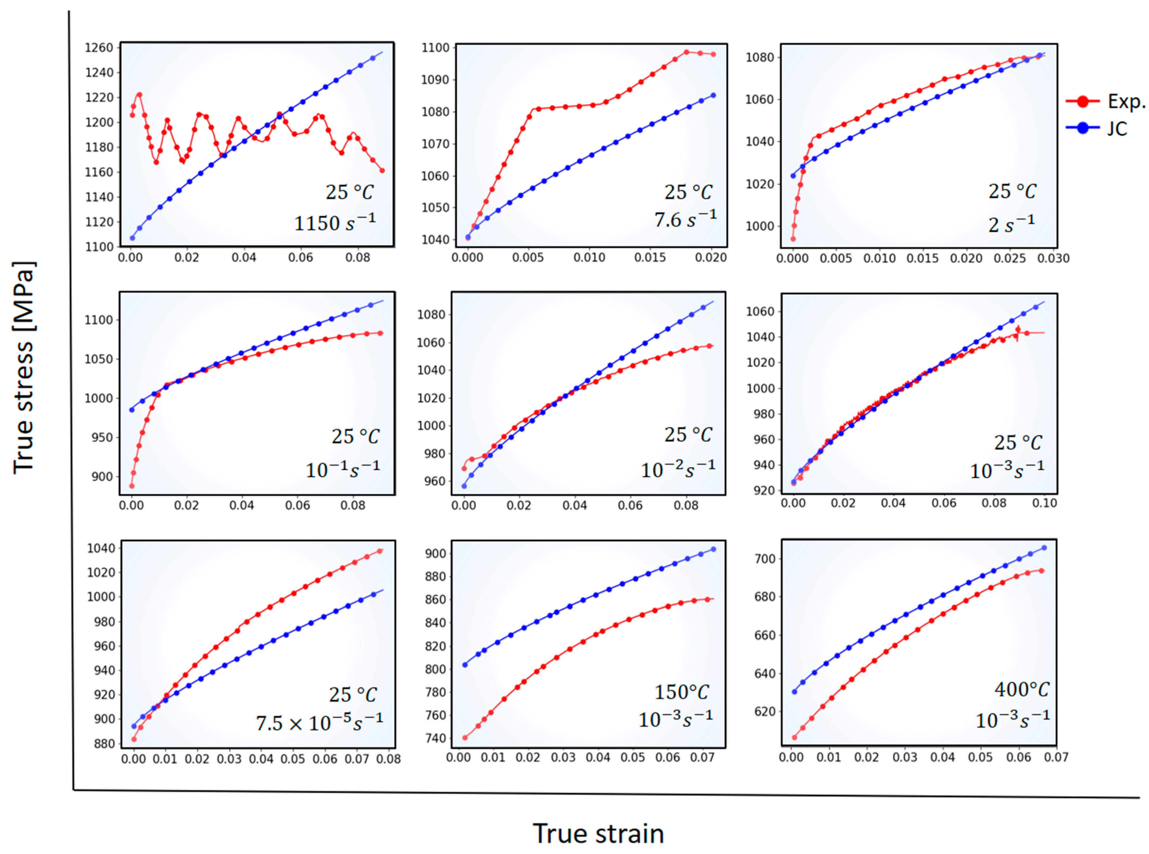
Experimental data demonstrate the reported strong effect of the temperature, and the strain rates’ effect on the strength of the Ti64 alloy is clearly observed. The increase of strain rate increases the value of stress in the alloy. The initial yield stress of the alloy captured between at 25 °C and at very low and high strain rated performed in the samples are between 881 and 1220 MPa. The stress rapidly decreases with the increase of the temperature for all the investigated strain rates. Thermal softening of the alloy reaches the yield stress of 600 MPa at 400 °C at 0.001/s.

Table 5. Johnson–Cook plasticity constants of Ti64 obtained by the direct calibration method.

Model Constant	Values
A (MPa)	927
B (MPa)	877.96
C (-)	0.0137
m (-)	0.594
n (-)	0.795

shows the parameters of the Johnson–Cook plasticity model obtained by the direct method of simultaneous fitting of the model with the experimental data for all tests both at different strain rates and at various temperatures (150 °C and 400 °C).

With the identified constants, the stress provided by the Johnson–Cook plasticity model was obtained and compared with the data from the tests as shown in Figure 5. To assessed the identification, the mean average percentage error (MAPE) is computed using Equation (5). The mean average percentage error (MAPE) obtained for the different loading conditions are shown in

Table 6. Average errors between the results obtained experimentally and analytically from the tensile tests with the data obtained with the direct method. The global MAPE is 2.1%.

	$\mathbf{Strain} \mathbf{Rate} {(\mathbf{s}}^{-1})$	Temperature (°C)	Error (MAPE)
Constant temperature tests with variable speed	1150	25	3.31
	$7.6$	25	0.99
	$2$	25	0.48
	${10}^{-1}$	25	2.56
	${10}^{-2}$	25	1.31
	${10}^{-3}$	25	0.73
	$7.5\times {10}^{-5}$	25	2.67
Constant strain rate tests with variable temperature	${10}^{-3}$	150	4.62
	${10}^{-3}$	400	2.47

.

From the values of the tensile tests at the same temperature and different strain rates, the errors prediction of the Johnson–Cook model obtained in the different tests are within an acceptable range. Please note that the change of slope of experimental points for some curves is related to the initial yielding of the material. As post-processing is performed using the 0.2% offset method [72], initial yielding could include some uncertainties in the identification method. However, verification of the global error of 2.1% indicate that this this discrepancy is negligible. In general, it was observed that the Johnson–Cook model for the Ti64 titanium alloy can be used to predict the stress in a wide range of strain rate. It is well known that this model is generally used for high speed deformations of metals and alloys, however, for the investigated Ti64, accurate predictions are obtained in full strain rate range (from ${10}^{-5}$ to ${10}^3 { \mathrm{s}}^{-1}$), demonstrating the applicability of this model for quasi-static a mid-range strain rate. For the results of the higher temperature, 150 °C and 400 °C, good results are also obtained in terms of model prediction with errors within an acceptable range (lower than 5% for all cases).

4.2. Johnson–Cook Damage Parameters by Direct Method

The resulting geometry parameters, cross-section radius $\left(a\right)$ and notch radius $\left(R\right)$ obtained with the digital image correlation post-processed in the current study is the input data to determine the stress triaxiality ($\eta$) of the specimens using the Bridgman method (Figure 6). The stress triaxiality and the dependent variables of the specimens computed with the method are shown in

Table 7. Stress triaxiality obtained with the Bridgman method, experimental fracture deformation, and fracture strain with the Johnson-Cook damage law at reference temperature and strain rate for the analyzed specimens. The global average error found is 3.4%.

Sample	Bridgman’s Stress Triaxiality	Experimental Fracture Strain	Johnson-Cook Fracture Strain	MAPE (%)
Cylindrical	0.416	0.518	0.517	0.23
R 3.5	0.499	0.306	0.319	4.10
R 5	0.59	0.290	0.263	9.20
R 4	0.696	0.242	0.250	2.80
R 2.5	0.783	0.247	0.247	0.07
R 1.5	1.093	0.236	0.246	4.19

. In addition, the value of the error between the experimental notch curve and that obtained by the aforementioned method is added.

The experimental fracture strain (${\epsilon }_f$) is calculated with the true strain definition depending on the initial $\left(A_0\right)$ and fractured ${(A}_f)$ cross-sections of the tensile sample (Equation (18)).

$${\epsilon }_f=\ln \left(\frac{A_0}{A_f}\right)$$

(18)

The triaxiality of the stress state in terms of principal components (${\sigma }_1, {\sigma }_2, \mathrm{a}\mathrm{n}\mathrm{d} {\sigma }_3)$ is defined as the ratio between the hydrostatic stress $\left(p\right)$ and the von Mises equivalent stress $\overline{(\sigma })$[73,74]. The mathematical form is given in Equation (19).

$$\eta =\frac{p}{\overline{\sigma }}=\frac{\frac{1}{3}\left({\sigma }_1+{\sigma }_2+{\sigma }_3\right)}{\sqrt{\frac{1}{2}\left({\left({\sigma }_1-{\sigma }_2\right)}^2+{\left({\sigma }_2-{\sigma }_3\right)}^2+{\left({\sigma }_3-{\sigma }_1\right)}^2\right)}}$$

(19)

The results of fracture strain obtained from the stress triaxiality using the Johnson-Cook damage law (Equation (3)) for reference temperature and strain rate are shown in Table 7.

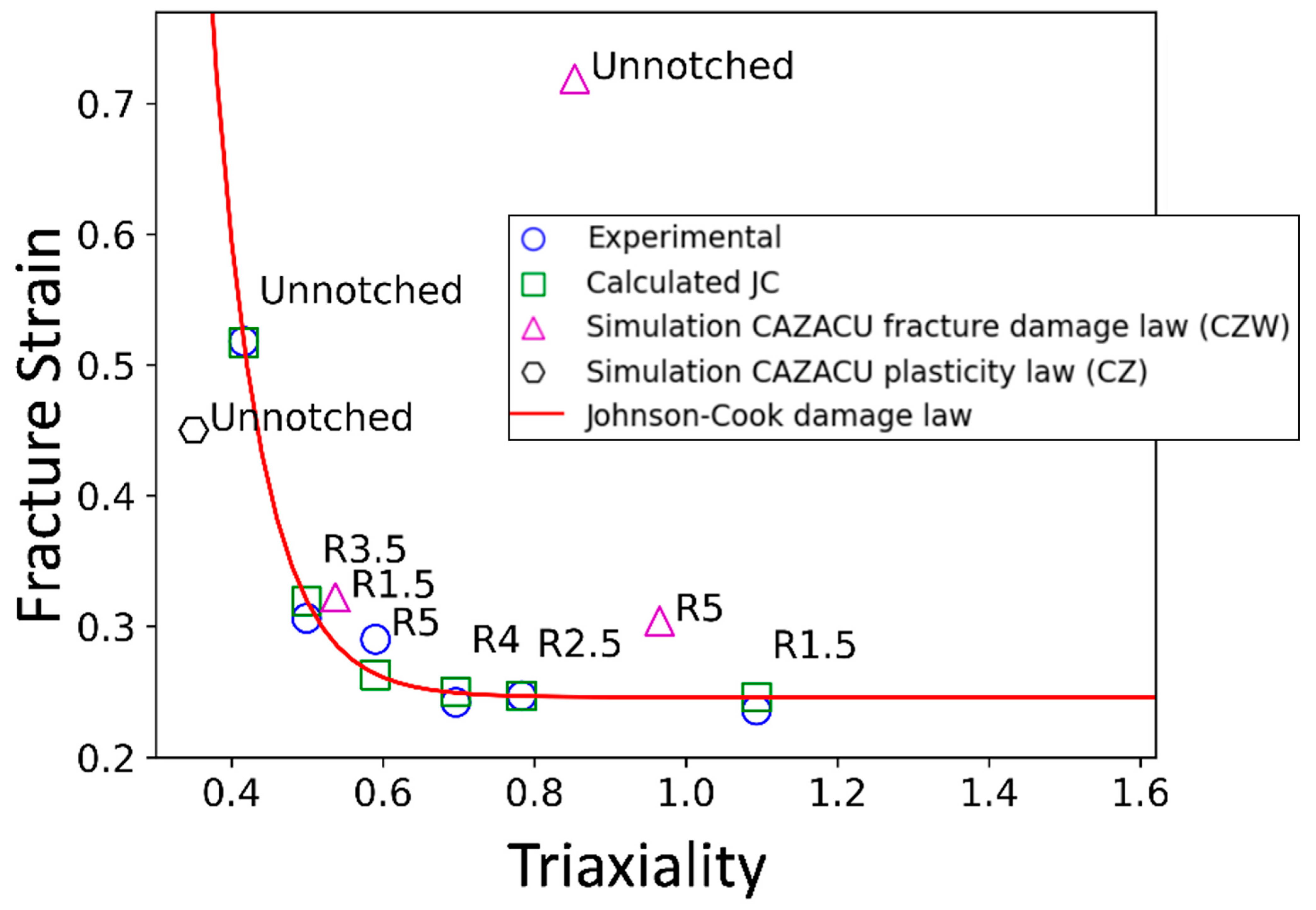
The relationship between the fracture deformation and the stress triaxiality of the investigated specimens is shown in Figure 7. This figure includes the data obtained from experimental stress triaxiality found with the Bridgman method and the data obtained through simulations with the SC11–TNT damage law previously reported in the literature [69]. The results of the micromechanics-based numerical simulation (SC11–TNT) match the local values of fracture deformation and stress triaxiality in the area where the fracture first appears. These simulated tests correspond to the tensile of specimens without a notch, specimens with a notch radius of 5 mm (R5), and specimens with a notch radius of 1.5 mm (R1.5). Note that local values computed in the damage law for smooth specimens are not average value of the samples, explaining the larger fracture strain. In addition, as notch localized deformation and produce a non-homogeneous stress triaxiality, the value locally does not correspond to average JC values. The law of plasticity without damage (CAZACU) for the specimen without notch is included to validate previous analysis, showing closeness to the predicted JC model. The experimental and simulation values compared with the evolution of the fracture deformation as a function of the stress triaxiality given by the Johnson-Cook damage model (Equation (10)) allows to determine the values for $d_1, d_2$ and $d_3$ through the direct identification method (

Table 8. Johnson Cook damage constants $d_1, d_2$ and $d_3$ for Ti64.

Parameters	Values
$d_1$	0.246
$d_2$	186.0
$d_3$	−15.7

) explained in Section 3.

4.3. Johnson–Cook Damage-Related Constants by Inverse Analysis

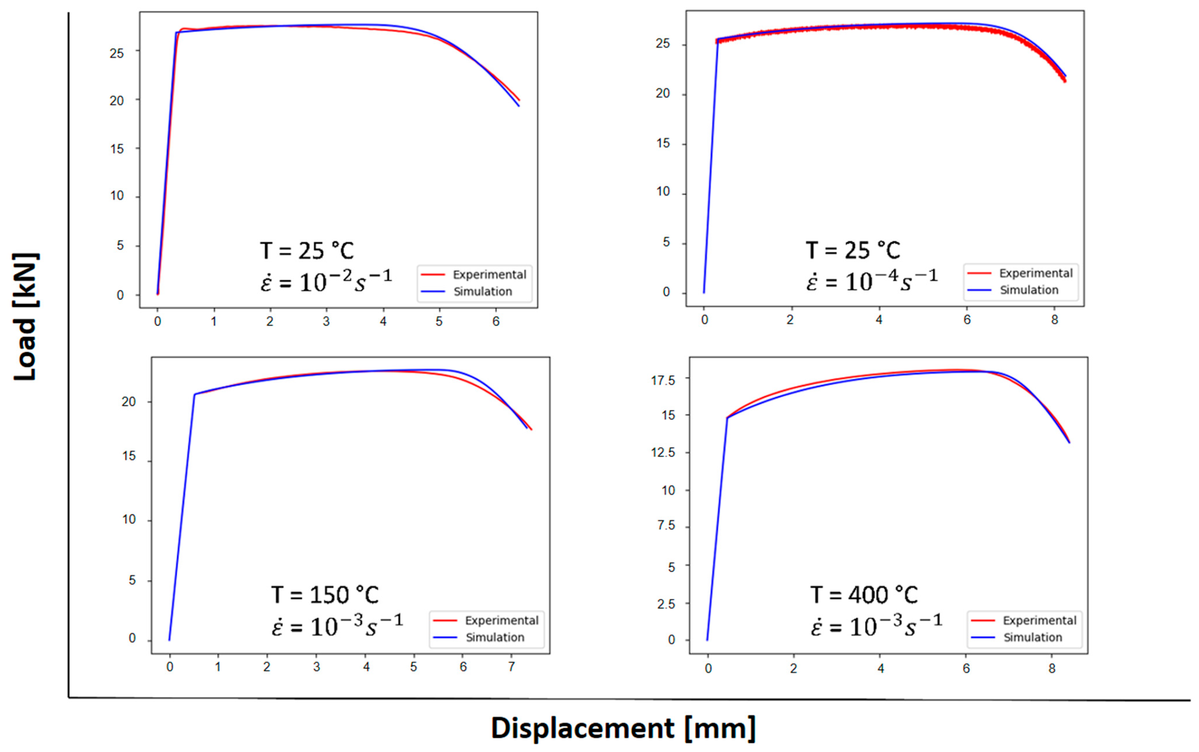
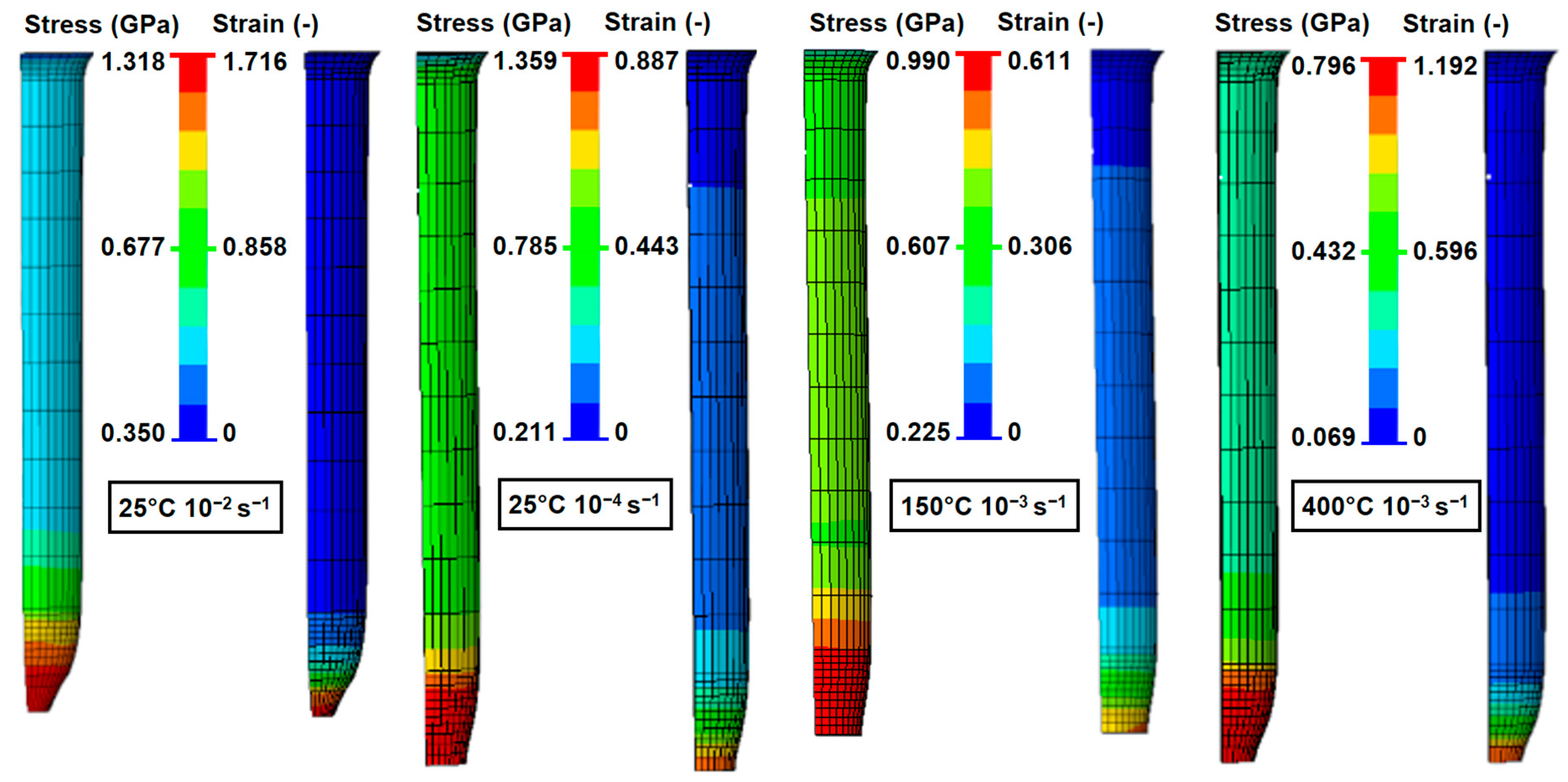
The results of experimental tests are adjusted to various temperatures and strain rates using the inverse analysis technique. The force-displacement results obtained by the simulations and compared with the experimental results are shown in Figure 8.

The mean absolute percentage error (MAPE) between the experimental and simulated curves was calculated using Equation (5), and the values obtained are shown in

Table 9. Percentage error between the experimental and simulated curves of the tensile tests at room temperature with different strain rates and tensile tests with constant strain rate and different temperatures.

Tensile Test	Temperature (°C)	$\mathbf{Strain} \mathbf{Rate} {(\mathbf{s}}^{-1})$	MAPE (%)
1	25	${10}^{-2}$	1.27
2	25	${10}^{-4}$	1.15
3	150	${10}^{-3}$	1.41
4	400	${10}^{-3}$	1.31

.

As can be seen, the errors calculated between the experimental curves and simulations have a value close to 1%. Consequently, the data obtained through the simulations can be correctly used to determine the damage parameters $d_4$ and $d_5$.

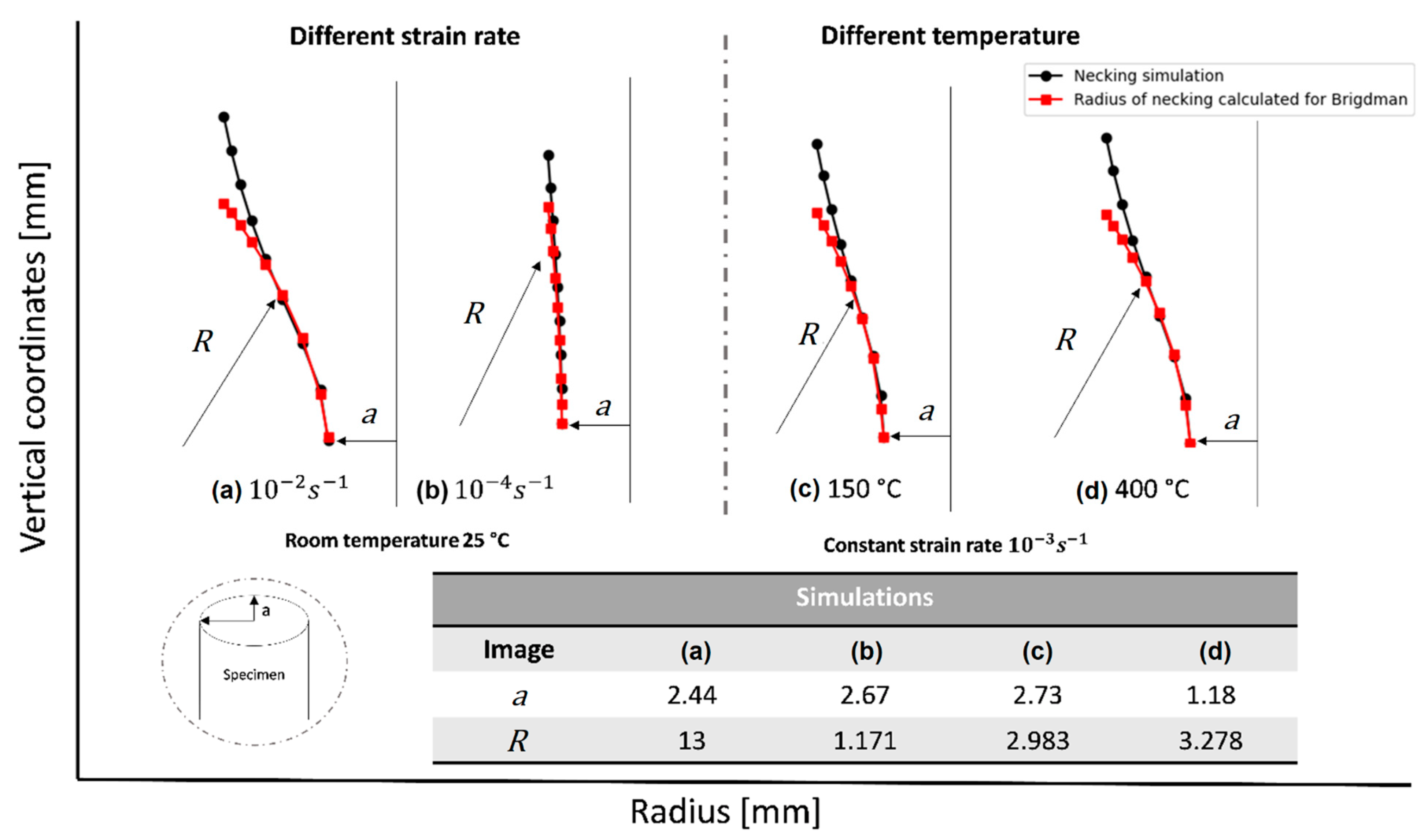
The values of the average radius of the cross-section ($a$) and vertical radius of the necking ($R$) of the tensile specimens are obtained from the validated simulations (Figure 9). These test variables required to calculate the stress triaxiality using the Bridgman method are shown in Figure 10.

Table 10. Triaxialities obtained with the Bridgman method using data from the different simulated tests.

Temperature (°C)	$\mathbf{Strain} \mathbf{Rate} {(\mathbf{s}}^{-1})$	Sample Stress Triaxiality
25	${10}^{-2}$	0.410
25	${10}^{-4}$	0.355
150	${10}^{-3}$	0.409
400	${10}^{-3}$	0.415

shows the stress triaxiality for each specimen computed with the Bridgman method and the data generated from the simulations. Finally,

Table 11. Damage constant $d_4$ and $d_5$ Johnson–Cook damage law obtained with the inverse method.

Parameters	Values
$d_4$	0.2582
$d_5$	1.2059

completes the damage-model-calibrated constants with the computed values of parameter $d_4$ and $d_5$ using the inverse method and linear regression from Equations (16) and (17).

4.4. Potential Implications of Identified JC Model for Aerospace Engineering Design and Manufacturing Optimization

The Johnson–Cook (JC) model constants provided in this work are essential in aerospace engineering design and the manufacturing optimization of aerospace titanium-grade parts. By utilizing finite element simulations and numerical optimization techniques, the model proposed for the Ti64 aerospace-grade titanium alloy can offer various benefits across a wide range of applications within the aerospace and medical industry, particularly for reducing costs associated with material testing and prototyping, leading to more efficient and cost-effective solutions.

In aerospace engineering design, the calibrated JC model can enhance the development of critical components such as aircraft engine components, fasteners, brackets, blades, discs, and structural airframe elements. By accurately predicting the behavior of the alloy under a wide range of operating conditions, engineers could optimize the design of these components for improved performance, durability, and safety. For aeronautical structures, including wing structures, landing gear components, and critical fasteners, the optimization of these components could improve impact resistance and overall aircraft safety. Through finite element simulations, engineers can also gain more accurate insights into the physical behavior of titanium-grade parts, leading to more reliable predictions and improved structural integrity, decreasing the overall workload and fuel consumption.

In the manufacturing optimization of aerospace titanium-grade parts such as springs, hydraulic tubing, engines, rotorcraft, and hydraulic system components, by utilizing numerical optimization and finite element modeling of several fabrication techniques, manufacturers can speed up the production process of defect-free parts while ensuring performance requirements. Moreover, this Johnson–Cook model could provide engineers with a deeper understanding of the alloy behavior for a more accurate predictions performance of the parts under various operating conditions, allowing for the development of more efficient and reliable aerospace components, and ultimately contributing to advancements in aerospace technology and safety standards. In conclusion, the application of the Johnson–Cook model constants of Ti64 has the potential to decrease workload, improve fuel consumption, enhance safety and impact resistance, and expedite the manufacturing process through precise knowledge of alloy behavior and accurate predictions of aerospace and aeronautical parts a wide range of operating conditions.

4.4.1. Limitations of the Study

Understanding the limitations of the identified Johnson–Cook model for the calibrated Ti64 alloys is critical to optimizing aerospace component design and manufacturing. This JC calibrated model assumes isotropic criteria for initial yielding under multiple stress conditions, as well as isotropic hardening neglecting any anisotropic response. In addition, this JC damage model cannot predict the different damage mechanism of void appearance or coalescence in comparison to micromechanics based models. However, in this work, this material complexity of multiple damage mechanisms is adequately represented for microscopic fracture of samples with average stress triaxiality of 0.4 and 1.1. The required accuracy for engineering design of a specific application determines the limitations of the Johnson–Cook model’s effectiveness. In this work, this model is limited for the very accurate design of bulk Ti64 aerospace parts manufactured from ingots, plates or bars, under temperature between 25 °C and 400 °C and under loading producing large strain rates in the range of ${10}^{-5}$ s⁻¹ and ${10}^3 { \mathrm{s}}^{-1}$. Material deformation of parts loaded out of this range will predict the behavior with higher error than the reported 2.1% in plasticity and 3.4% in fracture, and estimations of extrapolated behavior must be verified with adequate validation experiments. For instance, specific applications or design requirements for which the Johnson–Cook model may not adequately capture are cryogenic applications or machining with strain rate higher than ${10}^3 { \mathrm{s}}^{-1}$.

The Johnson–Cook model could also present limitations when applied to other aerospace-grade titanium alloy products. The model calibrated parameters may vary with process conditions, affecting the accuracy of predictions, especially if material experiences high strain rates and temperatures. For instance, if sheet aerospace-grade titanium alloy materials are analyzed and optimized for products design and manufacturing in different scenarios, a new identification and calibration could be needed. Previous deformation process during manufacturing can also modify the aerospace-grade titanium properties, such as ductility and toughness. The key limitation of this model lies in the assumption of strain hardening, strain rate hardening, and thermal softening as independent phenomena. This could lead to a model which may not fully capture the complex behavior of the aerospace-grade titanium alloys under extreme conditions. In this study, the unknown behavior occurs in the range below 25° or above 400 °C, as well as for creep loadings and ultra-high strain rates above ${10}^3 { \mathrm{s}}^{-1}$.

The practical significance of the calibrated SC11–TNT model for prediction the fracture of sample in a very accurate way lies in the capability of the model to predict fracture and local porosity due to void nucleation, growth, and coalesce. This micromechanical model has a great potential to not only predict initial failure, but also crack growth in a micro-, meso-, and macro-length scale for life cycle analysis and fatigue predictions of load-carrying Ti64 components under various conditions. However, further implementations and validation in commercial or in-house software is required.

4.4.2. Potential Future Directions

In the context of advancing aerospace engineering design and manufacturing optimization, the implications of the identified model for the safe design of aircraft engine components subjected to impact loads and the related optimization of manufacturing processes is highlighted. Manufacturing optimizations could be related to any part of aerospace-grade Ti64 alloy, including femoral implant or prosthesis owing to the biocompatibility capacity of the alloy. The parts subjected to impact load or critical components could fail under certain conditions. To avoid catastrophic and generalized failure of aircrafts, local damage of parts and components should be accurately predicted and plastic deformation programed to determine the corresponding design safety factor. This could include critical components such as aircraft engine parts, fasteners, brackets, blades, discs, springs, and hydraulic system components, among others. Plastic deformations respond differently according to the speed of the deformation process and temperature. In the case of fan blade out [75] or bird strike [76] of turbofan, engines are designed to contain the detachment of a blade from both the fan and turbines without perforation of the casing. With this identified model, the dynamic loads and deformations can be accurately predicted in the investigated ranges. Furthermore, with the identified Johnson–Cook model, manufacturing of Ti64 aerospace components or even for femoral implant manufacturing, trial and error virtual testing and customized design can be efficiently optimized through finite element-based numerical simulations techniques for large deformations.

5. Conclusions

This work correctly applies the proposed hybrid calibration strategy for fully determine the Johnson–Cook plasticity and damage laws for the Ti64 alloy using most of the data documented in various open literature sources. Based on the results analysis, the following statements are declared:

• The direct method allows the correct identification of the parameters of the Johnson–Cook plasticity law with the data obtained from tensile tests at different strain rates up to temperatures of 400 °C. The global mean average percentage error obtained by the plasticity model is 2.1%, which is very accurate for the design and optimization of aerospace components of Ti64 alloy under plastic deformation.
• The hydrostatic stress related parameters of the Johnson–Cook damage law, $d_1$, $d_2$, and $d_3$, are accurately adjusted with the evolution of the fracture deformation as a function of stress triaxiality. Considering an adequate safety factor of design, these parameters can be used for modeling fracture of structures and aerospace components of Ti64 at low speed and 25 °C.
• The mean absolute percentage errors (MAPE) between experimental and simulated curves of specimens with different states of stress triaxiality and deformed at various temperatures and strain rates are close to 1%. These results indicate that it is valid and appropriate to apply the finite element method with the calibrated SC11–TNT model to determine predictions of stress triaxiality and fracture strain required to calibrate parameters $d_4$ and $d_5$ of the Johnson–Cook damage law.
• The combined direct-inverse identification method yields a calibrated JC model with accurate predictions of the load-carrying capacity of Ti64 components, including material damage caused by loading under a wide range of strain rate between ${10}^{-5}$ to ${10}^3 { \mathrm{s}}^{-1}$ and temperatures below 400 °C.

Recent research is centered on assessing the efficacy of the established model in designing aircraft engine components that endure impact loads resulting in substantial deformations and material fracture. Furthermore, ongoing efforts are directed towards refining the manufacturing of femoral implants through impact forging and chip removal processes.

References

1. Pavlenko, D.; Dvirnyk, Y.; Przysowa, R. Advanced materials and technologies for compressor blades of small turbofan engines. Aerospace 2021, 8, 1. [Google Scholar] [CrossRef]
2. Miko, T.; Petho, D.; Gergely, G.; Markatos, D.; Gacsi, Z. A Novel Process to Produce Ti Parts from Powder Metallurgy with Advanced Properties for Aeronautical Applications. Aerospace 2023, 10, 332. [Google Scholar] [CrossRef]
3. Williams, J.C.; Boyer, R.R. Opportunities and Issues in the Application of Titanium Alloys for Aerospace Components. Metals 2020, 10, 705. [Google Scholar] [CrossRef]
4. Tuninetti, V.; Jaramillo, A.F.; Riu, G.; Rojas-Ulloa, C.; Znaidi, A.; Medina, C.; Mateo, A.M.; Roa, J.J. Experimental Correlation of Mechanical Properties of the Ti-6Al-4V Alloy at Different Length Scales. Metals 2021, 11, 104. [Google Scholar] [CrossRef]
5. Rojas-Ulloa, C.; Bouffioux, C.; Jaramillo, A.F.; García-Herrera, C.M.; Hussain, T.; Duchêne, L.; Riu, G.; Josep Roa, J.; Flores, P.; Marie Habraken, A.; et al. Nanomechanical Characterization of the Deformation Response of Orthotropic Ti–6Al–4V. Adv. Eng. Mater. 2021, 23, 2001341. [Google Scholar] [CrossRef]
6. Canale, G.; Kinawy, M.; Maligno, A.; Sathujoda, P.; Citarella, R. Study of mixed-mode cracking of dovetail root of an aero-engine blade like structure. Appl. Sci. 2019, 9, 3825. [Google Scholar] [CrossRef]
7. Wang, J.; Hu, X.; Yuan, K.; Meng, W.; Li, P. Impact resistance prediction of superalloy honeycomb using modified Johnson–Cook constitutive model and fracture criterion. Int. J. Impact Eng. 2019, 131, 66–77. [Google Scholar] [CrossRef]
8. Seddik, R.; Rondepierre, A.; Prabhakaran, S.; Morin, L.; Favier, V.; Palin-Luc, T.; Berthe, L. Identification of constitutive equations at very high strain rates using shock wave produced by laser. Eur. J. Mech.-A/Solids 2022, 92, 104432. [Google Scholar] [CrossRef]
9. Liu, G.; Zhang, D.; Yao, C. A modified constitutive model coupled with microstructure evolution incremental model for machining of titanium alloy Ti–6Al–4V. J. Mater. Process. Technol. 2021, 297, 117262. [Google Scholar] [CrossRef]
10. Che, J.; Zhou, T.; Liang, Z.; Wu, J.; Wang, X. An integrated Johnson–Cook and Zerilli–Armstrong model for material flow behavior of Ti–6Al–4V at high strain rate and elevated temperature. J. Brazilian Soc. Mech. Sci. Eng. 2018, 40, 253. [Google Scholar] [CrossRef]
11. Ahmad, D.; Kumar, D.; Ajaj, R.M. Multiaxial Deformations of Elastomeric Skins for Morphing Wing Applications: Theoretical Modeling and Experimental Investigations. Polymers 2022, 14, 4891. [Google Scholar] [CrossRef] [PubMed]
12. Gour, S.; Ahmad, D.; Kumar, D.; Ajaj, R.M.; Zweiri, Y. Investigating the Tear Fracture of Elastomeric Skins in Morphing Wings: An Experimental and Computational Study. Int. J. Appl. Mech. 2023, 15, 2350096. [Google Scholar] [CrossRef]
13. Mirzaie, T.; Mirzadeh, H.; Cabrera, J.M. A simple Zerilli-Armstrong constitutive equation for modeling and prediction of hot deformation flow stress of steels. Mech. Mater. 2016, 94, 38–45. [Google Scholar] [CrossRef]
14. Huang, S.; Khan, A.S. Modeling the mechanical behaviour of 1100-0 aluminum at different strain rates by the bodner-partom model. Int. J. Plast. 1992, 8, 501–517. [Google Scholar] [CrossRef]
15. Fameso, F.; Desai, D.; Kok, S.; Newby, M.; Glaser, D. Simulation of laser shock peening on X12Cr steel using an alternate computational mechanical threshold stress plasticity model. Int. J. Adv. Manuf. Technol. 2020, 111, 1–11. [Google Scholar] [CrossRef]
16. Nemat-Nasser, S.; Guo, W.G. Thermomechanical response of HSLA-65 steel plates: Experiments and modeling. Mech. Mater. 2005, 37, 379–405. [Google Scholar] [CrossRef]
17. Kotkunde, N.; Deole, A.D.; Gupta, A.K.; Singh, S.K. Comparative study of constitutive modeling for Ti-6Al-4V alloy at low strain rates and elevated temperatures. Mater. Des. 2014, 55, 999–1005. [Google Scholar] [CrossRef]
18. Johnson, G.R.; Cook, W.H. A constitutive model and data for metals subjected to large strains, high strain rates and high. In Proceedings of the 7th International Symposium on Ballistics, The Hague, The Netherlands, 19–21 April 1983; pp. 541–547. [Google Scholar]
19. Citarella, R.; Giannella, V.; Vivo, E.; Mazzeo, M. FEM-DBEM approach for crack propagation in a low pressure aeroengine turbine vane segment. Theor. Appl. Fract. Mech. 2016, 86, 143–152. [Google Scholar] [CrossRef]
20. Giannella, V.; Vivo, E.; Mazzeo, M.; Citarella, R. FEM-DBEM approach to simulate crack propagation in a turbine vane segment undergoing a fatigue load spectrum. Procedia Struct. Integr. 2018, 12, 479–491. [Google Scholar] [CrossRef]
21. Kay, G.J. Failure Modelling of Titanium 6Al-4V and Aluminum 2024-T3 With the Johnson-Cook Material Model, U.S. Department of Transportation, Federal Aviation Administration, Office of Aviation Research, Washington, DC 20591; pp. 1–24. Available online: https://www.tc.faa.gov/its/worldpac/techrpt/ar03-57.pdf (accessed on 14 March 2024).
22. Ojal, N.; Cherukuri, H.P.; Schmitz, T.L.; Devlugt, K.T.; Jaycox, A.W. A combined experimental and numerical approach that eliminates the non-uniqueness associated with the Johnson-Cook parameters obtained using inverse methods. Int. J. Adv. Manuf. Technol. 2022, 120, 2373–2384. [Google Scholar] [CrossRef]
23. Chen, G.; Ke, Z.; Ren, C.; Li, J. Constitutive modeling for Ti-6Al-4V alloy machining based on the SHPB tests and simulation. Chin. J. Mech. Eng. (Engl. Ed.) 2016, 29, 962–970. [Google Scholar] [CrossRef]
24. Kumar Reddy Sirigiri, V.; Yadav Gudiga, V.; Shankar Gattu, U.; Suneesh, G.; Mohan Buddaraju, K. A review on Johnson Cook material model. Mater. Today Proc. 2022, 62, 3450–3456. [Google Scholar] [CrossRef]
25. Murugesan, M.; Jung, D.W. Johnson cook material and failure model parameters estimation of AISI-1045 medium carbon steel for metal forming applications. Materials 2019, 12, 609. [Google Scholar] [CrossRef]
26. Farhadzadeh, F.; Salmani-Tehrani, M.; Tajdari, M. Determining biaxial tensile stresses by fracture cruciform specimen at different temperatures and strain rates for Ti–6Al–4V alloy. J. Braz. Soc. Mech. Sci. Eng. 2018, 40, 532. [Google Scholar] [CrossRef]
27. Kuliiev, R.; Keller, S.; Kashaev, N. Identification of Johnson-Cook material model parameters for laser shock peening process simulation for AA2024, Ti–6Al–4V and Inconel 718. J. Mater. Res. Technol. 2024, 28, 1975–1989. [Google Scholar] [CrossRef]
28. Tserpes, K.; Papadopoulos, K.; Unaldi, S.; Berthe, L. Development of a numerical model to simulate laser-shock paint stripping on aluminum substrates. Aerospace 2021, 8, 233. [Google Scholar] [CrossRef]
29. Wang, X.; Shi, J. Validation of Johnson-Cook plasticity and damage model using impact experiment. Int. J. Impact Eng. 2013, 60, 67–75. [Google Scholar] [CrossRef]
30. Neuvonen, R.; Skriko, T.; Björk, T. Use of the quasi-static Johnson-Cook model in the failure assessment of tensile specimens with metallurgical constraints. Eur. J. Mech.-A/Solids 2020, 82, 104011. [Google Scholar] [CrossRef]
31. Tuninetti, V.; Forcael, D.; Valenzuela, M.; Mart, A.; Medina, C.; Pincheira, G.; Salas, A.; Oñate, A.; Duch, L. Assessing Feed-Forward Backpropagation Artificial Neural Networks for Strain-Rate-Sensitive Mechanical Modeling. Materials 2024, 17, 317. [Google Scholar] [CrossRef]
32. Shi, L.; Wang, T.; Wang, L.; Liu, E. Research on Johnson–Cook Constitutive Model of γ-TiAl Alloy with Improved Parameters. Materials 2023, 16, 6715. [Google Scholar] [CrossRef]
33. Zhou, J.; Ren, J.; Jiang, Y. Inverse identification of modified Johnson–Cook model for cutting titanium alloy Ti6Al4V using firefly algorithm. Proc. Inst. Mech. Eng. Part B J. Eng. Manuf. 2020, 234, 584–599. [Google Scholar] [CrossRef]
34. Zhu, S.; Liu, J.; Deng, X. Modification of strain rate strengthening coefficient for Johnson-Cook constitutive model of Ti6Al4V alloy. Mater. Today Commun. 2021, 26, 102016. [Google Scholar] [CrossRef]
35. Song, W.; Ning, J.; Mao, X.; Tang, H. A modified Johnson–Cook model for titanium matrix composites reinforced with titanium carbide particles at elevated temperatures. Mater. Sci. Eng. A 2013, 576, 280–289. [Google Scholar] [CrossRef]
36. Valoppi, B.; Bruschi, S.; Ghiotti, A.; Shivpuri, R. Johnson-Cook based criterion incorporating stress triaxiality and deviatoric effect for predicting elevated temperature ductility of titanium alloy sheets. Int. J. Mech. Sci. 2017, 123, 94–105. [Google Scholar] [CrossRef]
37. Huang, Y.; Ji, J.; Lee, K.M. An improved material constitutive model considering temperature-dependent dynamic recrystallization for numerical analysis of Ti-6Al-4V alloy machining. Int. J. Adv. Manuf. Technol. 2018, 97, 3655–3670. [Google Scholar] [CrossRef]
38. Yang, S.; Liang, P.; Gao, F.; Song, D.; Jiang, P.; Zhao, M.; Kong, N. The Comparation of Arrhenius-Type and Modified Johnson–Cook Constitutive Models at Elevated Temperature for Annealed TA31 Titanium Alloy. Materials 2023, 16, 280. [Google Scholar] [CrossRef] [PubMed]
39. Rojas-Ulloa, C.; Valenzuela, M.; Tuninetti, V.; Habraken, A.M. Identification and validation of an extended Stewart-Cazacu micromechanics damage model applied to Ti–6Al–4V specimens exhibiting positive stress triaxialities. Proc. Inst. Mech. Eng. Part L J. Mater. Des. Appl. 2021, 235, 1248–1261. [Google Scholar] [CrossRef]
40. Tuninetti, V.; Flores, P.; Valenzuela, M.; Pincheira, G.; Medina, C.; Duchêne, L.; Habraken, A.M. Experimental characterization of the compressive mechanical behaviour of Ti6Al4V alloy at constant strain rates over the full elastoplastic range. Int. J. Mater. Form. 2020, 13, 709–724. [Google Scholar] [CrossRef]
41. Simha, C.H.M.; Williams, B.W. Modeling failure of Ti–6Al–4V using damage mechanics incorporating effects of anisotropy, rate and temperature on strength. Int. J. Fract. 2016, 198, 101–115. [Google Scholar] [CrossRef]
42. Rajaraman, D.; Hertelé, S.; Fauconnier, D. A novel calibration procedure of Johnson-Cook damage model parameters for simulation of scratch abrasion. Wear 2023, 528–529, 204977. [Google Scholar] [CrossRef]
43. Zhao, Z.; Ji, H.; Zhong, Y.; Han, C.; Tang, X. Mechanical Properties and Fracture Behavior of a TC4 Titanium Alloy Sheet. Materials 2022, 15, 8589. [Google Scholar] [CrossRef] [PubMed]
44. Hou, X.; Liu, Z.; Wang, B.; Lv, W.; Liang, X.; Hua, Y. Stress-strain curves and modified material constitutive model for Ti-6Al-4V over thewide ranges of strain rate and temperature. Materials 2018, 11, 938. [Google Scholar] [CrossRef] [PubMed]
45. Yan, L.; Jiang, A.; Li, Y.; Qiu, T.; Jiang, F.; Xie, H.; Wang, F.; Wu, X.; Zhang, Y. Dynamic constitutive models of Ti-6Al-4V based on isothermal ture stress–strain curves. J. Mater. Res. Technol. 2022, 19, 4733–4744. [Google Scholar] [CrossRef]
46. Tuninetti, V.; Oñate, A.; Valenzuela, M.; Sepúlveda, H.; Pincheira, G.; Medina, C.; García-Herrera, C.; Duchêne, L.; Habraken, A.M. Characterization approaches affect asymmetric load predictions of hexagonal close-packed alloy. J. Mater. Res. Technol. 2023, 26, 5028–5036. [Google Scholar] [CrossRef]
47. Aranda, P.M.; García-Herrera, C.; Celentano, D.; Tuninetti, V.; Toro, S.A.; Landeros, F. Hybrid numerical–experimental strategy for damage characterization of SAE 1045 steel. Eur. J. Mech.-A/Solids 2024, 103, 105169. [Google Scholar] [CrossRef]
48. Xinjian, L.; Guigen, Y.; Zhimin, W.; Shifeng, X.; Yi, Z. Optimization on the Johnson-Cook parameters of Ti-6Al-4V used for high speed cutting simulation. J. Phys. Conf. Ser. 2020, 1653, 012034. [Google Scholar] [CrossRef]
49. Gross, A.J.; Ravi-Chandar, K. Prediction of ductile failure in Ti–6Al–4V using a local strain-to-failure criterion. Int. J. Fract. 2016, 198, 221–245. [Google Scholar] [CrossRef]
50. Ayed, Y.; Germain, G.; Ammar, A.; Furet, B. Thermo-mechanical characterization of the Ti17 titanium alloy under extreme loading conditions. Int. J. Adv. Manuf. Technol. 2017, 90, 1593–1603. [Google Scholar] [CrossRef]
51. Tuninetti, V.; Gilles, G.; Flores, P.; Pincheira, G.; Duchêne, L.; Habraken, A.-M. Impact of distortional hardening and the strength differential effect on the prediction of large deformation behavior of the Ti6Al4V alloy. Meccanica 2019, 54, 1823–1840. [Google Scholar] [CrossRef]
52. Peirs, J.; Verleysen, P.; Van Paepegem, W.; Degrieck, J. Determining the stress–strain behaviour at large strains from high strain rate tensile and shear experiments. Int. J. Impact Eng. 2011, 38, 406–415. [Google Scholar] [CrossRef]
53. Lecarme, L. Viscoplasticity, Damage, and Fracture of Ti-6Al-4V. Ph.D. Thesis, Université catholique de Louvain, Ottignies-Louvain-la-Neuve, Belgium, 2013. [Google Scholar]
54. Tuninetti, V. Experimental and Numerical Study of the Quasi-Static Behavior of Ti–6Al–4v. Ph.D. Thesis, Univertisé de Liège, Liège, Belgium, 2014. [Google Scholar]
55. Peirs, J. Experimental Charcterisation and Modelling of the Dynamic Behaviour of the Titanium Alloy Ti6Al4V. Ph.D. Thesis, Ghent University, Gent, Belgium, 2012. [Google Scholar]
56. Tao, Z.-J.; Fan, X.-G.; Yang, H.; Ma, J.; Li, H. A modified Johnson–Cook model for NC warm bending of large diameter thin-walled Ti–6Al–4V tube in wide ranges of strain rates and temperatures. Trans. Nonferrous Met. Soc. China (Engl. Ed.) 2018, 28, 298–308. [Google Scholar] [CrossRef]
57. Gao, S.; Sang, Y.; Li, Q.; Sun, Y.; Wu, Y.; Wang, H. Constitutive modeling and microstructure research on the deformation mechanism of Ti-6Al-4V alloy under hot forming condition. J. Alloys Compd. 2022, 892, 162128. [Google Scholar] [CrossRef]
58. Farahani, H.K.; Ketabchi, M.; Zangeneh, S. Determination of Johnson–Cook Plasticity Model Parameters for Inconel718. J. Mater. Eng. Perform. 2017, 26, 5284–5293. [Google Scholar] [CrossRef]
59. Verleysen, P.; Peirs, J. Quasi-static and high strain rate fracture behaviour of Ti6Al4V. Int. J. Impact Eng. 2017, 108, 370–388. [Google Scholar] [CrossRef]
60. Fylstra, D.; Lasdon, L.; Watson, J.; Waren, A. Design and use of the Microsoft Excel Solver. Interfaces 1998, 28, 29–55. [Google Scholar] [CrossRef]
61. Lasdon, L.; Fox, R.; Ratner, M. Nonlinear optimization using the generalized. Inform. Rech. Opérationn 1974, 3, 73–103. [Google Scholar]
62. Marquardt, D.W. An Algorithm for Least-Squares Estimation of Nonlinear Parameters. J. Soc. Ind. Appl. Math. 1963, 11, 431–441. [Google Scholar] [CrossRef]
63. Dang, N.; Luo, X.; Suo, T.; Dou, Q.; Ma, C.; Zhou, L. Damage evolution and failure in a titanium alloy: Revealed by 3D in situ X-ray tomography. J. Alloys Compd. 2022, 890, 161689. [Google Scholar] [CrossRef]
64. Li, X.; Cescotto, S. A mixed element method in gradient plasticity for pressure dependent materials and modelling of strain localization. Comput. Methods Appl. Mech. Eng. 1997, 144, 287–305. [Google Scholar] [CrossRef]
65. Simo, J.C.; Hughes, T.J.R. On the variational foundations of assumed strain methods. J. Appl. Mech. Trans. ASME 1986, 53, 51–54. [Google Scholar] [CrossRef]
66. Duchêne, L.; El Houdaigui, F.; Habraken, A.M. Length changes and texture prediction during free end torsion test of copper bars with FEM and remeshing techniques. Int. J. Plast. 2007, 23, 1417–1438. [Google Scholar] [CrossRef]
67. Harbaoui, R.; Daghfas, O.; Znaidi, A.; Tuninetti, V. Mechanical behavior of materials with a compact hexagonal structure obtained by an advanced identification strategy of HCP material, AZ31B-H24. Frat. Integrità Strutt. 2020, 14, 295–305. [Google Scholar] [CrossRef]
68. Gilles, G.; Tuninetti, V.; Ben Bettaïe, M.; Cazacu, O.; Habraken, A.M.; Duchene, L. Experimental characterization and constitutive modeling of TA6V mechanical behavior in plane strain state at room temperature. AIP Conf. Proc. 2011, 1383, 78–85. [Google Scholar] [CrossRef]
69. Rojas-Ulloa, C.; Tuninetti, V.; Sepúlveda, H.; Betaieb, E.; Pincheira, G.; Gilles, G.; Duchêne, L.; Habraken, A.M. Accurate numerical prediction of ductile fracture and micromechanical damage evolution for Ti6Al4V alloy. Comput. Mech. 2023, 73, 177–198. [Google Scholar] [CrossRef]
70. Tuninetti, V.; Gilles, G.; Milis, O.; Pardoen, T.; Habraken, A.M. Anisotropy and tension–compression asymmetry modeling of the room temperature plastic response of Ti–6Al–4V. Int. J. Plast. 2015, 67, 53–68. [Google Scholar] [CrossRef]
71. Tuninetti, V.; Habraken, A.M. Impact of anisotropy and viscosity to model the mechanical behavior of Ti-6Al-4V alloy. Mater. Sci. Eng. A 2014, 605, 39–50. [Google Scholar] [CrossRef]
72. Scholtz, D.; Wang, C.; English, M.; Mynors, D. Overcoming the Dependence of the Yield Condition on the Absence of Macroscopic Structures. Processes 2023, 11, 4. [Google Scholar] [CrossRef]
73. Peng, J.; Zhou, P.; Wang, Y.; Dai, Q.; Knowles, D.; Mostafavi, M. Stress triaxiality and lode angle parameter characterization of flat metal specimen with inclined notch. Metals 2021, 11, 1627. [Google Scholar] [CrossRef]
74. Hancock, J.W.; Mackenzie, A.C. On the mechanisms of ductile failure in high-strength steels subjected to multi-axial stress-states. J. Mech. Phys. Solids 1976, 24, 147–160. [Google Scholar] [CrossRef]
75. Sepúlveda, H.; Valle, R.; Pincheira, G.; Prasad, C.S.; Salas, A.; Medina, C.; Tuninetti, V. Dynamic numerical prediction of plasticity and damage in a turbofan blade containment test. Proc. Inst. Mech. Eng. Part L J. Mater. Des. Appl. 2022, 237, 2551–2560. [Google Scholar] [CrossRef]
76. Puneeth, M.L.; Jayaprakash, D. Influence of bird mass and impact height on the fan-blade of an aero-engine. Mater. Today Proc. 2021, 44, 1028–1038. [Google Scholar] [CrossRef]
Figure 1. FESEM micrograph view of the Ti64 alloy showing the heterogeneous distribution of α-/β phases [4].
Aerospace 11 00285 g001
Figure 2. Experimental tensile tests setup showing DIC cameras and necked-fractured sample.
Aerospace 11 00285 g002
Figure 3. Cylindrical and notch samples.
Aerospace 11 00285 g003
Figure 4. Mesh of one-eight geometry of cylindrical tensile sample simulated in different tests conditions of strain rates and temperatures using Cazacu plasticity and SC11–TNT damage models.
Aerospace 11 00285 g004
Figure 5. Comparison between the identified analytical model of Johnson–Cook plasticity and experimental stress–strain results in specimens deformed at different strain rates and temperatures [31,53,54,55,71].
Aerospace 11 00285 g005
Figure 6. Experimental notch at fracture obtained with the digital image correlation method and the adjusted value of radius (minimum cross-sectional radius a-value, and notch radius R in mm) for applying Bridgman method of stress triaxiality computation.
Aerospace 11 00285 g006
Figure 7. Relationship between fracture deformation and stress triaxiality among the experimental results, simulated with the CAZACU plasticity law, the CAZACU fracture damage law, and the Johnson-Cook damage law.
Aerospace 11 00285 g007
Figure 8. Comparison between experiments and simulations of stress–strain tensile tests at different strain rates for constant temperature (top), and tests at different temperatures and constant strain rates (bottom).
Aerospace 11 00285 g008
Figure 9. Notched-fractured sample from numerical simulations of tensile tests.
Aerospace 11 00285 g009
Figure 10. Notch of the specimens used for tensile tests at room temperature with different strain rates (a,b); and tests at different temperatures with identical strain rate (c,d). Note that the deformed sample is at the onset of rupture.
Aerospace 11 00285 g010