Remaining Useful Life Prediction for Aircraft Engines under High-Pressure Compressor Degradation Faults Based on FC-AMSLSTM

Abstract

The healthy operation of aircraft engines is crucial for flight safety, and accurate Remaining Useful Life prediction is one of the core technologies involved in aircraft engine prognosis and health management. In recent years, deep learning-based predictive methods within data-driven approaches have shown promising performance. However, for engines experiencing a single fault, such as a High-Pressure Compressor fault, existing deep learning-based predictive methods often face accuracy challenges due to the coupling relationship between different fault modes in the training dataset that includes a mixture of multiple fault modes. In this paper, we propose the FC-AMSLSTM method, a novel approach for Remaining Useful Life prediction specifically targeting High-Pressure Compressor degradation faults. The proposed method effectively addresses the limitations of previous approaches by fault classification and decoupling fault modes from multiple operating conditions using a decline index. Then, attention mechanisms and multi-scale convolutional neural networks are employed to extract spatiotemporal features. The long short-term memory network is then utilized to model RUL estimation. The experiments are conducted using the Commercial Modular Aero-Propulsion System Simulation dataset provided by NASA. The results demonstrate that compared to other prediction models, the FC-AMSLSTM method effectively reduces RUL prediction error for HPC degradation faults under multiple operating conditions.

1. Introduction

Prognostic and Health Management (PHM) has been used extensively in the automotive, marine, aviation, and other industries over the past decades. As opposed to conventional maintenance strategies, PHM aims to warn of failures before they occur, reduce the probability of serious disasters, and reduce repair costs [1]. Remaining Useful Life (RUL) forms an integral part of prognosis and health management and an important basis for judging the stability of equipment [2].

There are three approaches to predicting Remaining Useful Life (RUL) [3]: physical model-based approaches, hybrid approaches, and data-driven approaches. The physics-based approach for engine RUL prediction utilizes the engine’s physical characteristics and equations to establish a model. It predicts the RUL of the engine by monitoring and analyzing its operating conditions. Nathan Bolander et al. [4] presented a physics-based RUL prediction method for aircraft engine bearings, specifically targeting faults on the outer raceway. Matthew et al. [5] presented a physics-based prognostic method that considers the simultaneous occurrence of multiple damage processes within a component and applies it to system and component prognostic maintenance.

Hybrid approaches typically use statistical models as well as stochastic process models to simulate the degradation process of an aircraft engine and estimate RUL. Degeneracy-based approaches include, for example, the Weibull distribution [6] and degeneracy models based on nonlinear drifting Wiener processes [7]. There are also methods based on particle filtering [8]. However, aircraft engines are characterized by complex structures, making it challenging to establish accurate physical and mathematical models. This complexity arises from various factors such as fluid dynamics, combustion processes, heat transfer, and mechanical interactions within the engine.

Due to these complexities, accurately modeling the behavior of an aircraft engine becomes a daunting task. Uncertainties in factors like operating conditions, component degradation, and external influences further contribute to the limitation of prediction accuracy.

To address these challenges, data-driven approaches have gained popularity in the field of engine prediction and health monitoring. These approaches leverage machine learning and statistical techniques to learn patterns and relationships directly from the available data, bypassing the need for precise physical models.

The availability of data from aircraft engine sensors has become easier with the advancement of science and technology. As a result, researchers now have access to a substantial amount of data, enabling them to adopt a data-driven approach for predicting RUL. Early methods include Hidden Markov Model-based methods [9] and Support Vector Regression methods [10]. However, these methods required manual feature engineering, which could lead to inaccurate or incomplete feature selection. Moreover, these models performed poorly in handling complex non-linear relationships, making it difficult to capture the intricate features of engine degradation.

With the development of deep learning techniques, Recurrent Neural Networks (RNNs), attention mechanisms, convolutional neural networks (CNNs), and transformers have been proposed and applied to RUL prediction and fault diagnosis. Babu et al. [11] proposed a method for the predictive estimation of RUL using a CNN. However, the CNN ignores the temporal correlation of sensor state data. To overcome this problem, long and short-term memory (LSTM) networks have been invented [12]. KONG et al. [13] proposed a model fusing CNN and LSTM for RUL prediction.

Boujamza et al. [14] proposed a method for the prediction of RUL based on attention and LSTM. Liu et al. [15] proposed a double attention-based data-driven framework for aircraft engine RUL prognostics. Khumprom et al. [16] explored the current state of using deep neural networks for feature selection in data-driven prognostic models of aircraft engines. Zhang et al. [17] proposed a multilayer cross-domain transformer network to predict the RUL of rolling bearing. Zhang et al. [18] proposed an information stream fusion and semi-supervised learning method for intelligent fault diagnosis in offshore wind turbine bearings.

Xiang et al. [19] proposed a Bayesian Gated-Transformer (BGT) model for reliable RUL prediction in aircraft engines, utilizing the transformer architecture and a gated mechanism to balance long-term trends and short-term patterns. Zhang et al. [20] presented a pruning-adaptive optimal lightweight transformer to address the issue of redundant elements in the RUL prediction model for aerospace engines.

However, existing deep learning-based methods for engine RUL prediction neglect the impact of different engine failure modes on RUL prediction, especially when multiple failure modes and multiple operating conditions are coupled. Compared to single operating conditions and single failure modes, the prediction accuracy of existing methods significantly decreases in complex operating conditions. The challenges stated above arise from complex operating conditions, where engine data from various failure modes can overlap, leading to difficulties in accurately extracting relevant features for RUL fitting. This issue is further compounded by the presence of measurement noise, making the task even more challenging. Measurement noise in the engine system refers to the interference and errors in sensor measurements caused by various factors (such as sensor aging and electromagnetic interference), which may result in deviations or uncertainties between the sensor data and the actual engine state.

To address this issue, this paper proposes an FC-AMSLSTM model for RUL prediction of engine High-Pressure Compressor (HPC) degradation faults under multiple operating conditions. Firstly, a decline index is constructed based on the different trends of engine variations between different failure modes to differentiate HPC degradation faults from fan degradation faults. Based on the fault classification results, a dedicated dataset for HPC degradation faults is constructed. The AMSLSTM model is then used to predict the RUL of engines that have HPC degradation faults. The prediction model utilizes attention mechanisms to handle multiple operating conditions of the engine, employs multi-scale convolutional neural networks to extract spatial features at different time scales, and utilizes long short-term memory networks to capture temporal features. Finally, a fully connected layer is used to output the RUL value of the engine.

The approach of fault classification for engines in this paper contributes to improving the accuracy and reliability of RUL prediction. By categorizing engine failures into different classes, dedicated RUL prediction models can be established for different failure modes. This approach can better adapt to the actual working conditions and failure characteristics of the engine, enhancing the accuracy of RUL prediction.

This paper’s structure is as follows: Section 2 provides an overview of related work. Section 3 presents the methodology proposed in this paper. The experimental results are presented in Section 4. Finally, Section 5 concludes the paper and discusses future directions for the work.

2. Related Work

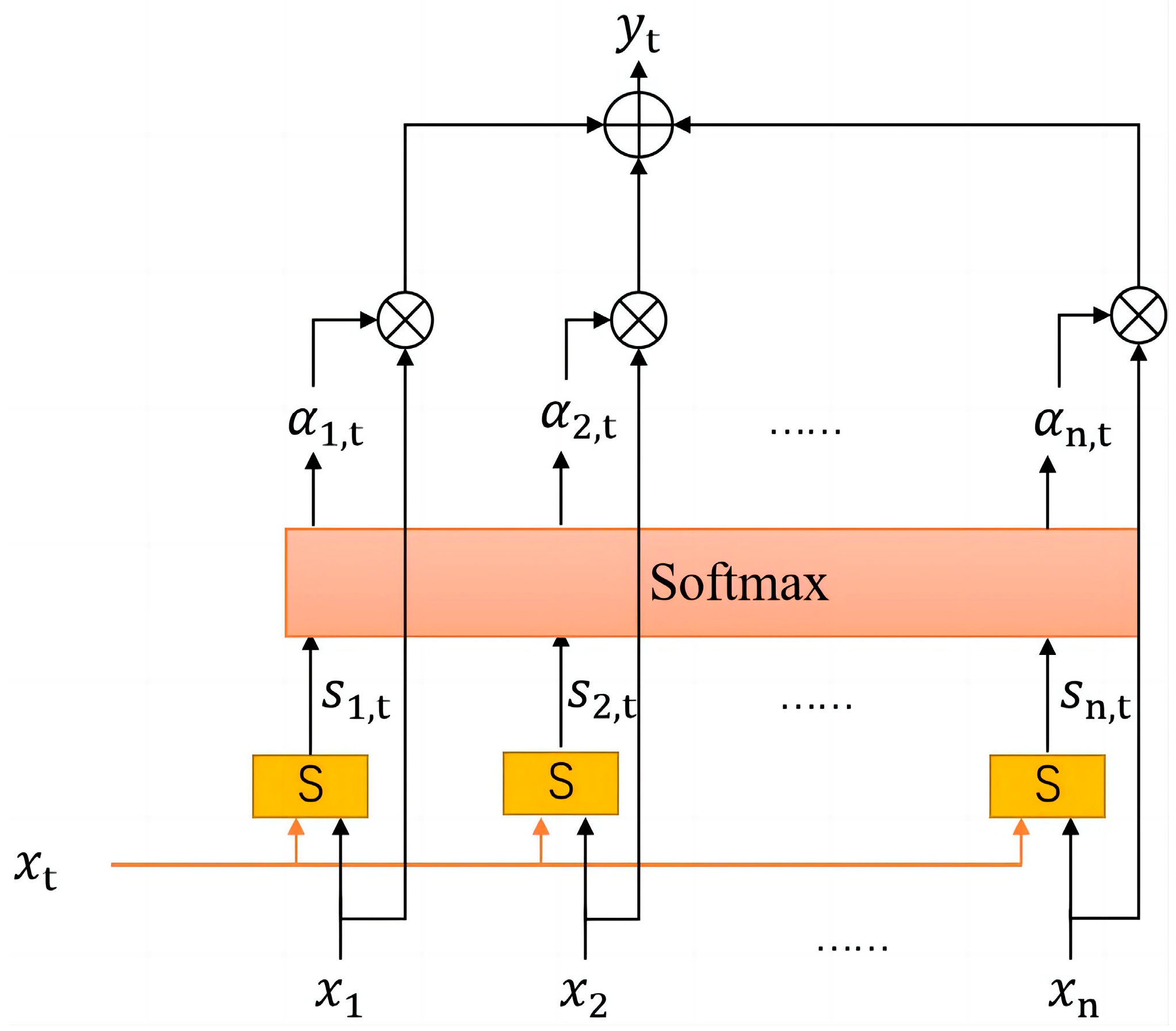
2.1. Attention Mechanism

The attention mechanism is a commonly used technique in machine learning and natural language processing, which mimics the human attention mechanism to address the relevance and importance between different parts of an input sequence [21].

In traditional machine learning models, all parts of the input sequence are typically treated equally. However, the attention mechanism allows the model to focus on specific parts of the input sequence, allocating more attention to those parts that are relevant to the current task. This mechanism enables the model to handle different parts of the input sequence flexibly, thereby improving the performance and representation of the model [22].

The core idea of the attention mechanism is to compute weights for each input part and apply these weights to the representation of the input sequence, generating a weighted sum representation. This weighted sum representation is then used as the output of the model or passed to the next layer for further processing. The weights of the attention mechanism are typically determined by calculating the relevance between each part of the input sequence and the current task. The structure of the attention mechanism is shown in Figure 1.

The processing flow of the attention mechanism can be described as follows:

$$s_{n,t}=S\left(x_n,x_t\right),$$

(1)

when calculating the network output $y_n$ for $x_n$, the first step is to compute the relevance scores $s_{n,t}$ between $x_n$ and the other input $x_t$ at different time steps $(t=1, 2, \dots , n)$. The $s_{n,t}$ represents the importance or similarity between $x_n$ and each $x_t$.

After computing the relevance scores $s_{n,t}$, they undergo a normalization process in order to standardize as follows:

$${\alpha }_{n,t}=Softmax\left(S\left(x_n,x_t\right)\right)=\frac{S\left(x_n,x_t\right)}{{\sum }_{j=1}^{i}S\left(x_j,x_t\right)}$$

(2)

The normalized relevance scores ${\alpha }_{n,t}$ are subsequently utilized to weigh the network inputs $x_t$. Each $x_t$ is multiplied by its corresponding normalized relevance score and then summed up to obtain the final network output $y_n$. This weighted-sum process allows the model to focus more on the inputs that are deemed more relevant or important for the current task.

$$y_t={\sum }_{\mathrm{j}=1}^n{\mathsf{\alpha }}_{j,\mathrm{t}}{\mathrm{x}}_j$$

(3)

Equations (4) and (5) represent the computations involved in calculating the relevance scores using a multi-layer perceptron (MLP) for the attention mechanism.

$$h_{n,t}=\tan h\left(x_n^T{W}_1+x_t^T{W}_1^{\prime }+b_1\right),$$

(4)

$$s_{n,t}=\sigma \left(W_2{h}_{n,t}+b_2\right),$$

(5)

where $h_{n,t}$ represents the hidden state or intermediate representation for the relevance computation between $x_n$ and $x_t$. It is calculated using a combination of the input vectors $x_n$ and $x_t$, along with learnable parameters $W_1$, $W_1^{\prime }$ and $b_1$. The $\tan h$ activation function is then applied to the resulting vector. $s_{n,t}$ represents the relevance score between $x_n$ and $x_t$. It is computed based on the hidden state $h_{n,t}$ obtained from Equation (4). The hidden state $h_{n,t}$ is passed through another linear transformation using the weight matrix $W_2$ and bias term $b_2$. This sigmoid function squashes the output to represent the relevance score.

By using an MLP to calculate the relevance scores, the model becomes more flexible in capturing complex relationships and can dynamically adjust the weights based on the specific task or context at hand. This allows the attention mechanism to adapt and focus on the most relevant parts of the input sequence, enhancing the model’s performance in capturing important information.

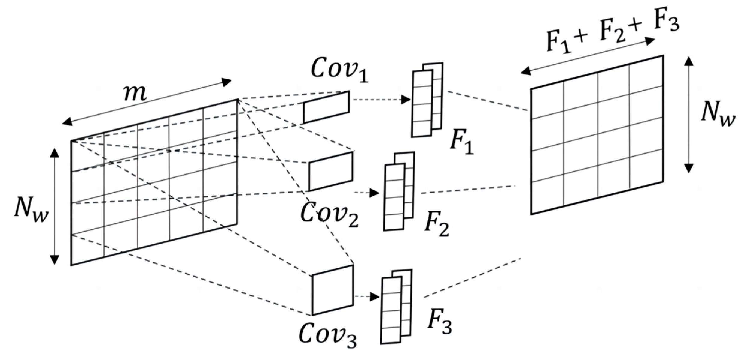
2.2. Multi-Scale Convolutional Neural Network

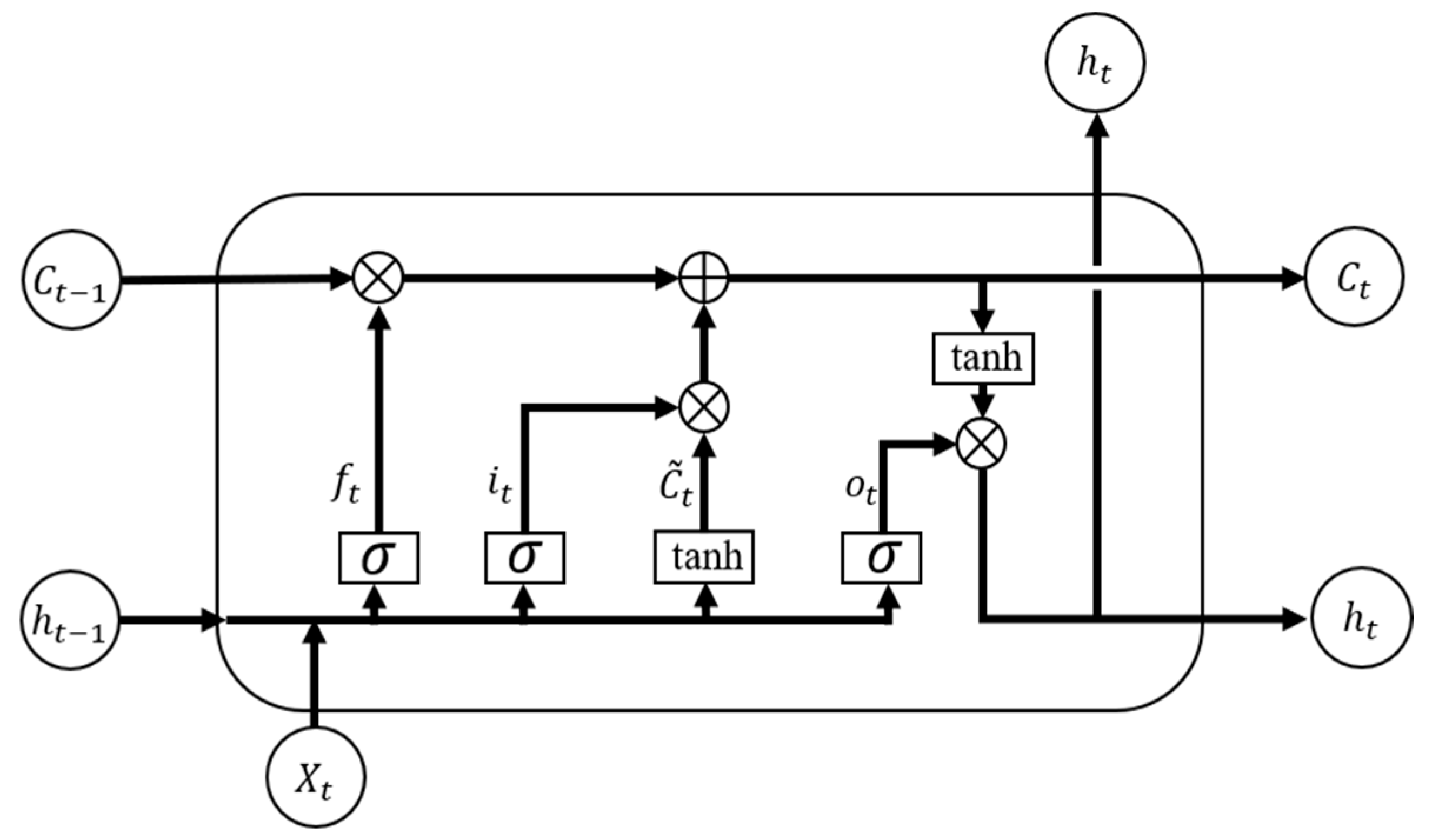
CNNs have strengths in processing high-dimensional data, and the original position relationship is still retained after the convolution operation. Therefore, CNNs are widely applied to feature extraction [23]. To avoid the effect of the change of engine sensor order on the prediction result, the 1-Dimensional (1D) convolution kernel is required. The width of the 1D convolution kernel is the same as the sample, while the length and amount of convolution kernels are artificially set as hyperparameters. However, a single-length 1D convolutional kernel is not sufficient to extract the complex degradation features of the engine, so the Multi-Scale Convolutional Neural Network (MSCNN) is necessary [24]. The structure of the MSCNN model is shown in Figure 2. $m$ and $N_w$ denote the width and length of the samples; $Cov1$, $Cov2$, and $Cov3$ are three different sizes of 1D convolution kernels; $F_1$, $F_2$, and $F_3$ are the amount of $Cov1$, $Cov2$, and $Cov3$ used.

Suppose the sample $S={\left[S_1,S_2,\dots ,S_{N_w}\right]}^T\in R^{N_w\times m}$; after convolution with a 1D convolution kernel $K_u$, the result is

$$h_u=\begin{array}{c}[\phi \left(W_u{S}_{1:t_u}+b_u\right),\phi \left(W_u{S}_{2:t_u+1}+b_u\right),\dots \phi \left(W_u{S}_{i:t_u+i-1}+b_u\right), \\ {\dots ,\phi \left(W_u{S}_{N_w-t_u+1:N_w}+b_u\right)]}^T\end{array}$$

(6)

where $S_{i:t_u+i-1}={\left[S_i,S_{i+1},\dots ,S_{t_u+i-1}\right]}^T;h_u$ is the output after the sample has been convolved by $K_u$; $\phi$ is the activation function of $K_u$; $W_u$, $b_u$ are the weights and biases of $K_u$, and $t_u$ is the kernel size of $K_u$.

The multiscale convolutional neural network is used to convolve the samples using several different sizes of thought convolutional kernels. The final result is obtained as

$$H=\left[h_1,h_2,\dots ,h_u,\dots h_n\right],$$

(7)

where $H$ is the output of the multiscale convolutional neural network, and $n$ is the total number of 1D convolutional kernels used.

It is worth noting that when the input data are processed using different sizes of convolutional kernels, the dimensionality of the obtained results is not consistent. Therefore, we need to use the padding method to ensure that the samples have the same dimensionality.

2.3. LSTM

The RNN has a ring structure and handles short-term memory well but is unable to perform long-term memory output. The LSTM adds a cellular state to the RNN, reducing the possibility of gradient disappearance and gradient explosion [25]. Figure 3 shows the structure of the LSTM cell.

The calculation formulas of the flow process in the LSTM cell block are as follows:

$$f_t=\sigma \left(b_f+U_f{x}_t+W_f{h}_{t-1}\right),$$

(8)

$$i_t=\sigma \left(b_i+U_i{x}_t+W_i{h}_{t-1}\right),$$

(9)

$${\tilde{C}}_t=\tan h\left(b_c+U_c{x}_t+W_c{h}_{t-1}\right),$$

(10)

$$C_t=f_t{C}_{t-1}+i_t{\tilde{C}}_t,$$

(11)

$$o_t=\sigma \left(b_o+U_i{x}_t+W_o{h}_{t-1}\right),$$

(12)

$$h_t=o_t\tan h\left(C_t\right),$$

(13)

where $\sigma$ is the sigmoid function; $W_f$, $W_i$, $W_c$, and $W_o$ are the loop weight of each layer; $U_f$, $U_i$, $U_c$, and $U_o$ are the input weight of each gate; and $b_f$, $b_i$, $b_c$, and $b_o$ are the bias. Equation (8) describes the output of the forget gate, which is used to control the discarding and retention of old information when new information is input. Equations (9) and (10) are the equations of the input gates. Firstly, the information of the hidden state of the previous layer and the current input are passed to the sigmoid function. Secondly, the information of the hidden state of the previous layer and the current input is passed to the tanh function, and finally, it is decided which information is important and should be kept. Equation (11) updates the cell state with the information obtained earlier. The final prediction results are obtained by Equations (12) and (13).

3. Method

3.1. The Experiment Dataset

Due to the harsh operating conditions of aircraft engine components, which are exposed to high temperatures and pressures, performance degradation is inevitable with increasing usage. It is crucial to obtain monitoring data from initial operation to failure in order to model and analyze the degradation process of the engine. However, for aircraft engines, which are highly expensive equipment, it is challenging to collect data through active usage of multiple real engines. The National Aeronautics and Space Administration (NASA) utilizes the MAPSS system to simulate the realistic deterioration of a turbofan engine [26]. The simulated model can generate a maximum thrust of 90,000 $\mathrm{l}\mathrm{b}$. In addition, the engine can work under different operating conditions, including differing altitudes, Mach numbers, and sea-level temperatures.

In the C-MAPSS dataset, 21 types of sensor data for aircraft engines are recorded. Their descriptions and units are shown in

Table 1. Description of the aircraft engine sensor measurements [27].

NO	Description	Units
1	Total temperature at fan inlet	$°\mathrm{R}$
2	Total temperature at LPC outlet	$°\mathrm{R}$
3	Total temperature at HPC outlet	$°\mathrm{R}$
4	Total temperature at LPT outlet	$°\mathrm{R}$
5	Pressure at fan inlet	psia
6	Total pressure in bypass duct	psia
7	Total pressure at HPC outlet	psia
8	Physical fan speed	rpm
9	Physical core speed	rpm
10	Engine pressure ratio (P50/P2)	-
11	Static pressure at HPC outlet	psia
12	Ratio of fuel flow to Ps30	pps/psi
13	Corrected fan speed	rpm
14	Corrected core speed	rpm
15	Bypass ratio	-
16	Burner fuel–air ratio	-
17	Bleed enthalpy	-
18	Demanded fan speed	rpm
19	Demanded corrected fan speed	rpm
20	HPT coolant bleed	lbm/s
21	LPT coolant bleed	lbm/s

. The engine health is reflected by monitoring the engine temperature, speed, pressure data, etc. RUL prognostic is based on the historical data of 21 engine sensors recorded in the CMAPSS dataset. RUL prediction in this study utilized data from all 21 sensors.

Table 2. C-MAPSS dataset description.

Dataset	FD001	FD002	FD003	FD004
Number of training engines	100	260	100	249
Number of test engines	100	259	100	248
Max/Min cycles for training engines	362/128	378/128	525/145	543/128
Max/Min cycles for test engines	303/31	367/21	475/38	486/19
Operating conditions	1	6	1	6
Fault modes	1	1	2	2

provides a comprehensive description of the C-MAPSS dataset, which consists of four dataset variants: FD001, FD002, FD003, and FD004.

The four sub-datasets differ from each other in terms of the operating conditions and fault modes. For instance, FD001 only has one operating condition and one fault mode (HPC degradation fault). FD004 involves engines operating under six different operating conditions, and the engines exhibit two fault modes (HPC degradation fault and fan degradation fault).

Each dataset in the C-MAPSS dataset comprises multiple multivariate time series. These datasets are then divided into separate training and test subsets. In the training set, the magnitude of the fault gradually increases until the system fails. In contrast, the time series in the test set ends some time before the system reaches failure. Each record includes 26 channels involving engine id, running time (in cycles), 3-dimensional operating condition setting, and 21-dimensional sensor readings.

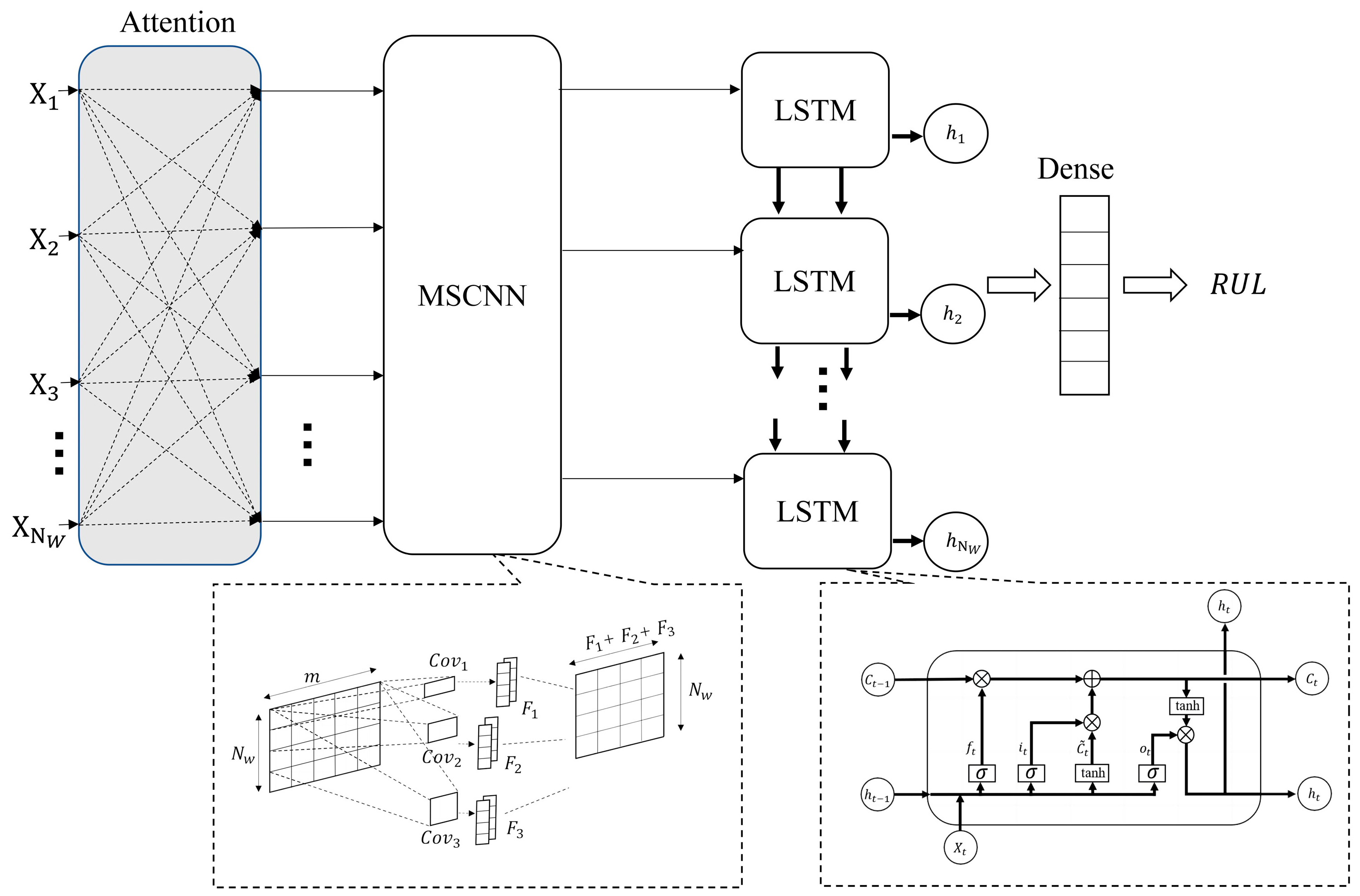
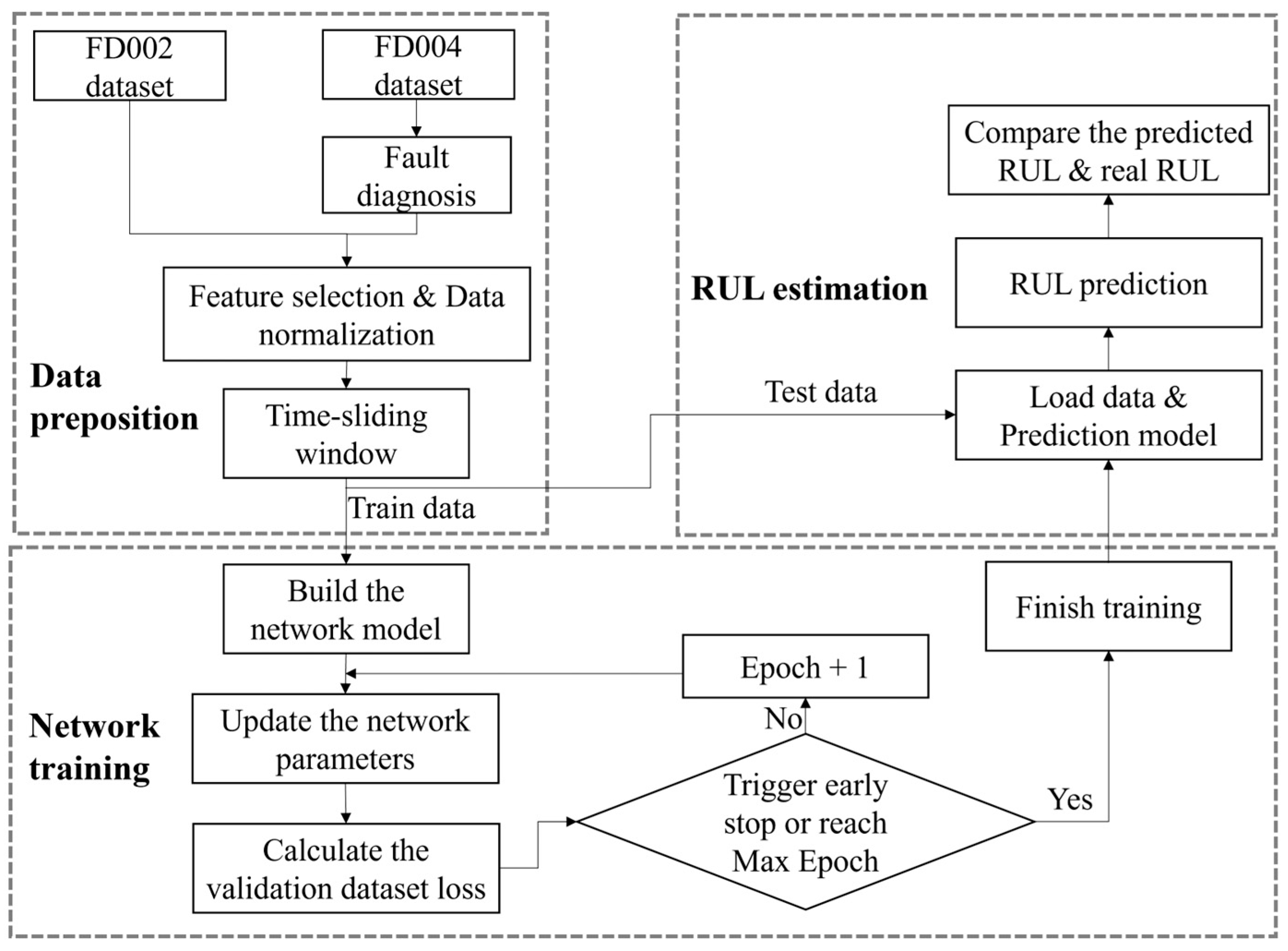
3.2. Prediction Process and Network Architecture

The network structure of the proposed method is shown in Figure 4. Firstly, the attention mechanisms are utilized to handle the multiple operating conditions of the engine. This attention mechanism helps to capture the varying dynamics and characteristics of the engine under different operating conditions. Secondly, the multi-scale CNN component extracts spatial features at different time scales. By applying convolutional filters of varying sizes, the model can capture both local and global patterns in the input data. Lastly, the LSTM networks are employed to capture temporal dependencies and patterns in the engine data. By utilizing memory cells and gates, LSTM networks can effectively model and remember long-term dependencies in the time-series data. This is particularly useful in RUL prediction tasks, where historical patterns and trends often play a crucial role in determining the remaining useful life of the engine.

During RUL prediction, each individual sample consists of 60 time steps of sensor data, denoted as $N_w=60$. At each time step, 21 sensor measurements of the engine, as shown in Table 1, are recorded. Therefore, the input size of the network is $(60\times 21)$, representing the sequence of sensor data over time. The attention mechanism is employed to extract relevant features by calculating the similarity between different time steps within a single sample. This mechanism allows the model to focus on important time steps or patterns in the sensor data, enhancing its ability to capture temporal dependencies and make accurate predictions for the remaining useful life.

In the field of aircraft engine RUL prediction, sensor data from different operating conditions may exhibit distinct patterns and behaviors. By applying the attention mechanism, the model can focus more on the features at the current time step that are similar to the target operating condition when processing the sensor data.

By calculating the similarity of features at different time steps, the attention mechanism provides a mechanism for the model to adaptively weigh the features at different time points, giving more importance to time steps that are similar to the target operating condition. This allows the model to capture the relevant features and patterns associated with the target operating condition more accurately, thereby improving the performance of RUL prediction.

The MSCNN component of the architecture is effective in extracting features at multiple scales. Different scales of features can provide complementary information and capture different aspects of the data. This helps in capturing both local and global patterns in the sensor data, enhancing the model’s ability to extract meaningful and discriminative features for RUL prediction. The LSTM component of the architecture is well-suited for modeling sequential data and capturing long-term dependencies. It can remember and utilize information from previous time steps, allowing the model to understand the temporal patterns and relationships in the sensor data.

By combining attention mechanisms, multi-scale CNN, and LSTM networks, the proposed model can effectively capture both spatial and temporal features, adapt to varying operating conditions, and make accurate predictions of the Remaining Useful Life of the engine. This integrated approach enhances the model’s ability to handle complex and dynamic degradation patterns, ultimately improving the accuracy and reliability of RUL predictions.

The experimental flow is shown in Figure 5. First, classify the data into different fault categories and extract the engine data diagnosed as HPC degradation fault to create training and testing datasets. Then, the engine sensor data need to be pre-processed, including normalization and sliding window. Normalization is used to eliminate the influence of different sensor data with different units on the prediction results. Sliding window is used to ensure that the input dimensions are consistent for each sample.

This is followed by network training. This consists of determining the network structure and parameters, updating the network weights using the training dataset, and outputting the prediction model. To prevent overfitting, this method uses early stopping. When the maximum iteration period is reached or the prediction error of the validation dataset does not decrease after 20 iterations, the model is suspended and outputs the final prediction model. Afterward, the test dataset is used to make the prediction, and the results are compared with the real RUL.

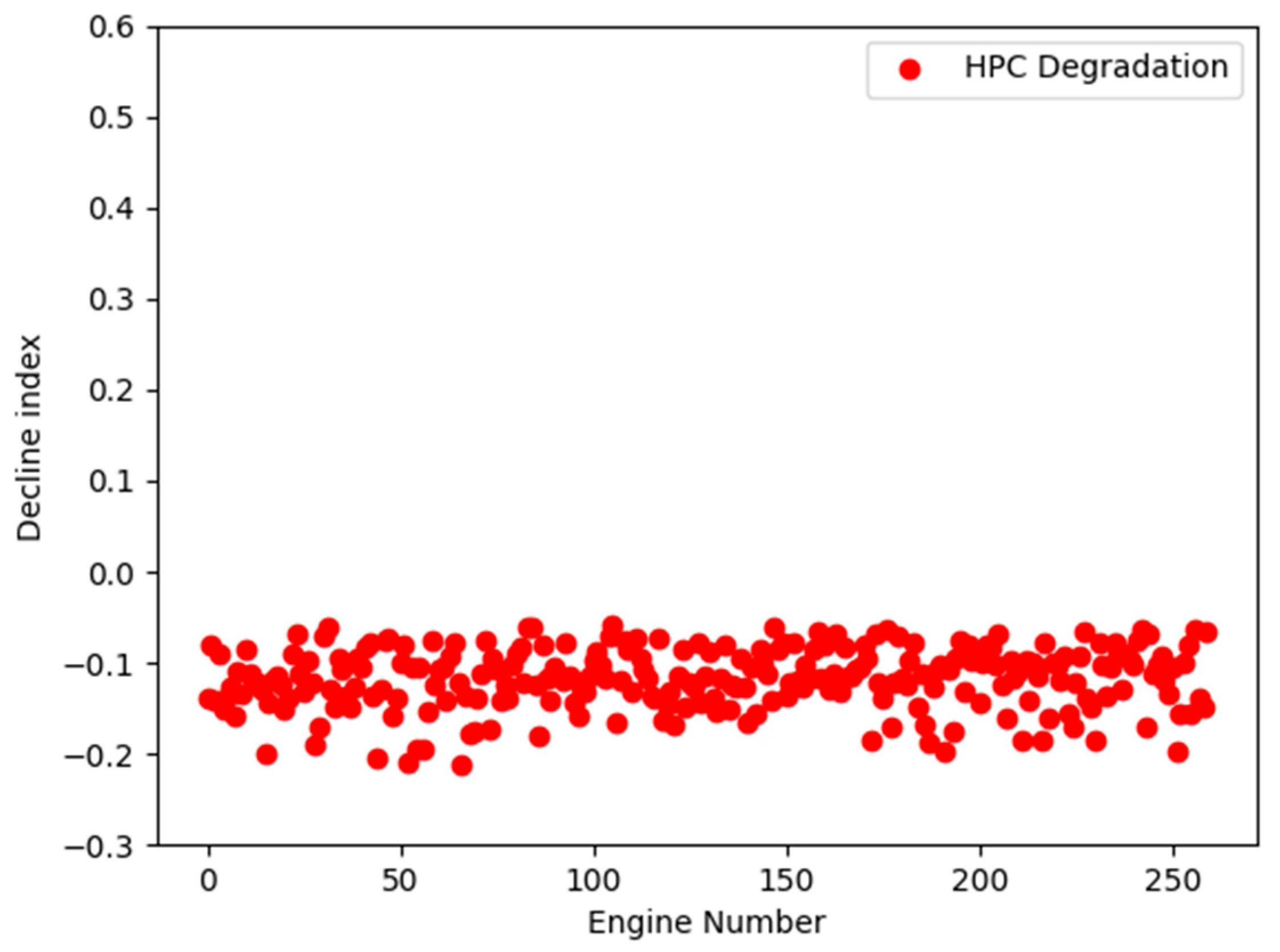
3.3. Fault Classification Method

The principle of the fault classification used in this study is that different fault modes may exhibit different trends in sensor data [28]. According to

Table 3. Operating condition classification.

Operating Conditions	Altitude (kft)	Mach Number	Sea-Level Temperature (°F)
Operating condition 1	0	0	100
Operating condition 2	10	0.25	100
Operating condition 3	20	0.7	100
Operating condition 4	25	0.62	60
Operating condition 5	35	0.84	100
Operating condition 6	42	0.84	100

, the engine operating conditions are classified into 6 categories based on altitude, Mach number, and sea-level temperature.

Figure 6 depicts the scatter plot of P30 (total pressure at HPC outlet) data for a specific engine before and after the classification of operating conditions. The x-axis represents the operating cycles, and the y-axis represents the P30 data. Each red dot in Figure 6 represents the recorded raw P30 data for the respective engine during the current operating cycle.

Figure 6a exhibits noticeable data discontinuities prior to performing operating condition classification.

Figure 6a illustrates the phenomenon of data discontinuities before the classification of operating conditions due to the changes in engine operating conditions throughout the operating cycles. It is difficult to observe any degradation trends. However, Figure 6b–e represent the scatter plots of P30 data for each individual operating condition after the classification. Upon conducting the operating condition classification, it becomes evident that the initially discontinuous data undergo a transformation into six scatter plots, each exhibiting a distinct degradation trend.

Following the classification of operating conditions, the FD002 and FD004 datasets were analyzed to observe data variations under specific operating conditions. The FD002 dataset represents a single fault mode, specifically HPC degradation, while the FD004 dataset includes two fault modes (HPC degradation fault and fan degradation fault). When examining the trend of sensor data changes for each dataset under a single operating condition, noticeable differences were observed.

Figure 7 and Figure 8 illustrate this comparison. Figure 7 displays the variation curves of BPR (bypass ratio) for all 260 engines in the FD002 training dataset under operating condition 1. Figure 8 shows the variation curves of BPR for all 249 engines in the FD004 training dataset under the same operating condition. The x-axis represents the operating cycles of the engine, while the y-axis represents the engine’s BPR values. The different colored lines in Figure 7 and Figure 8 represent the variations in BPR data for different engines under operating condition 1. Each line with a different color represents a different engine.

When classifying engine failures, the sensor data tends to exhibit abrupt changes due to variations in operating conditions at different time points. As shown in Figure 6a, however, when performing condition-based classification, significant trends can be observed in the data under a single operating condition without complex abrupt changes. Therefore, Figure 7 and Figure 8 illustrate the variations in BPR data for all engines in the FD002 and FD004 training datasets under a single operating condition. It can be observed that the BPR data in the FD002 training set only show an increasing trend, as it has only one fault mode. In contrast, the FD004 training dataset contains two fault modes, resulting in two distinct trends in the data. Based on this phenomenon, a decline index can be designed to differentiate between these two types of faults.

These observations suggest that this feature has the potential to distinguish between HPC (High-Pressure Compressor) degradation faults and fan degradation faults in engines. In addition to BPR data, the engine’s P30 and phi (ratio of fuel flow to Ps30) data were also employed for fault classification in this study.

The original data of the engine are denoted as $x_{ij}$, representing the $j$th sensor data of the engine in the $i$th operating cycle. After the classification of operating conditions, the original data are transformed into $x_{ij}^{n_i}$, where $n_i$ represents the operating condition for the engine in the $i$th operating cycle. Then, the change slope is calculated by performing a least-squares fit and summation of the different sensor data using Equation (14)

$${\alpha }_j={\sum }_{n_i=1}^6\frac{Cov(i_{n_i},x_{ij}^{n_i})}{Var\left(i_{n_i}\right)},$$

(14)

where ${\alpha }_j$ represents the slope and $i_{n_i}$ represents the set of operating cycles for the engine under operating condition $i_{n_i}$. Then, according to Equation (15), the decline index of different sensors in the engine is weighted and summed to obtain the final decay index.

$$\alpha ={\sum }_{j=1}^3{W}_j{\alpha }_j,$$

(15)

where $W_j$ represents the weight assigned to each sensor.

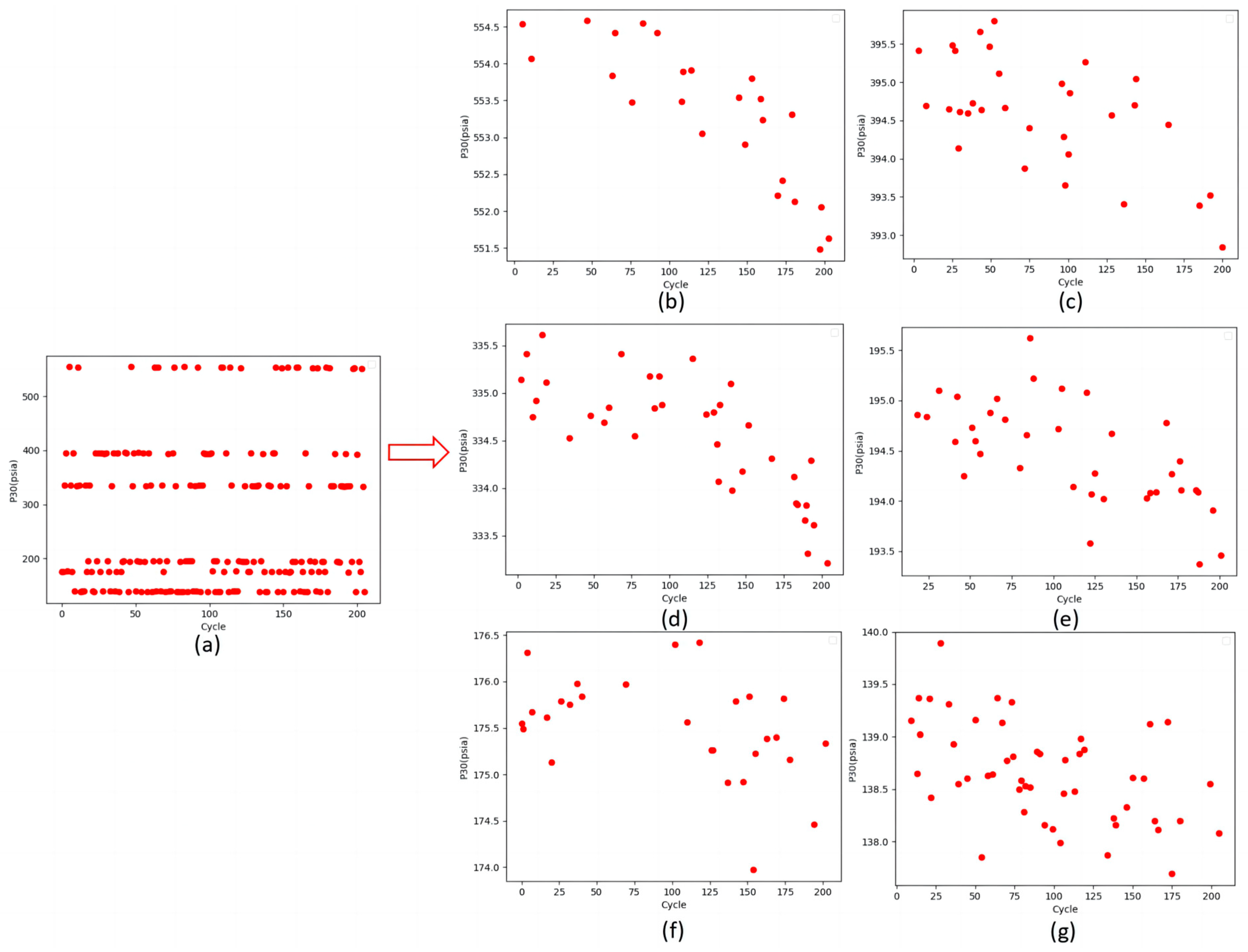
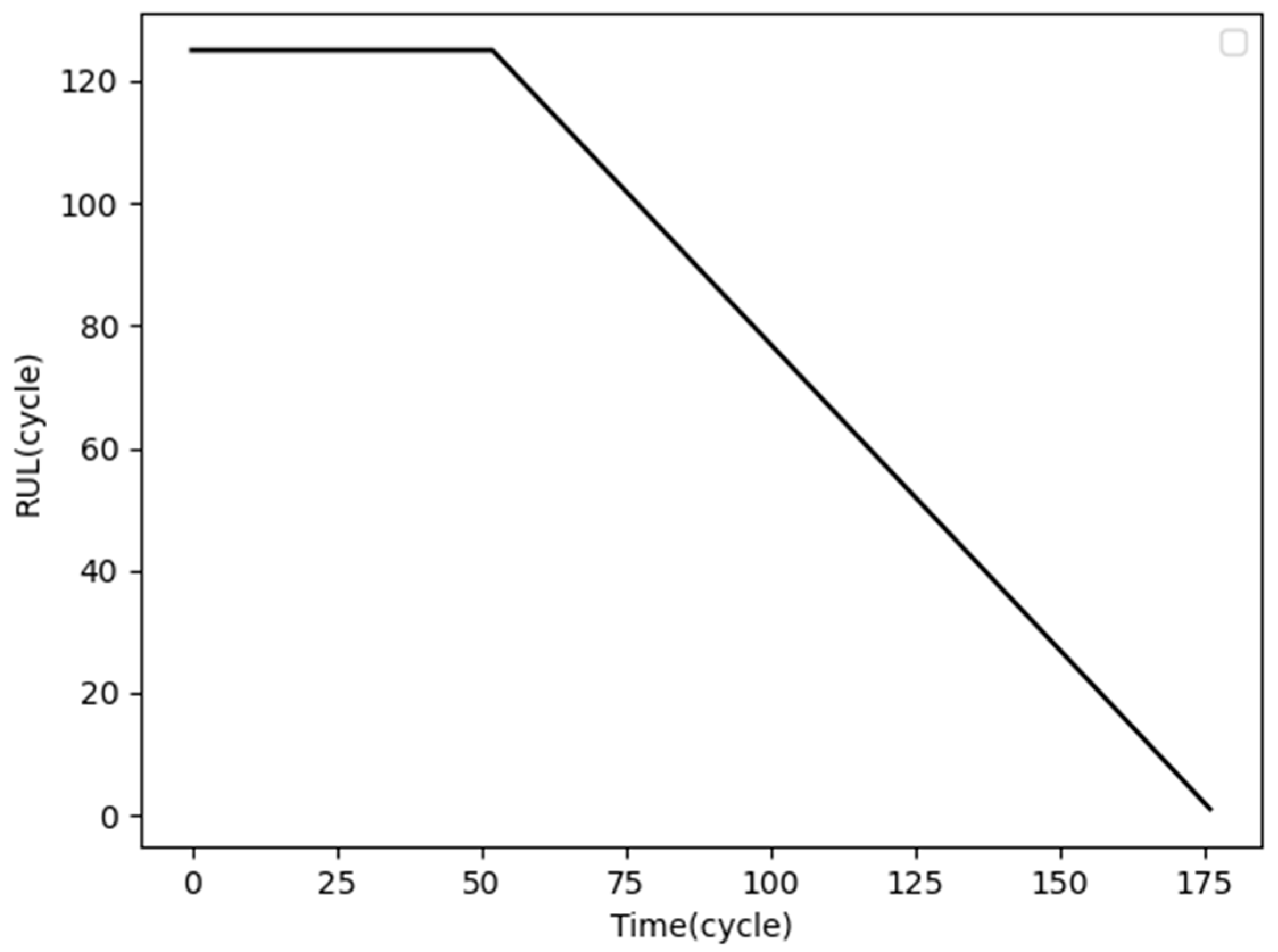
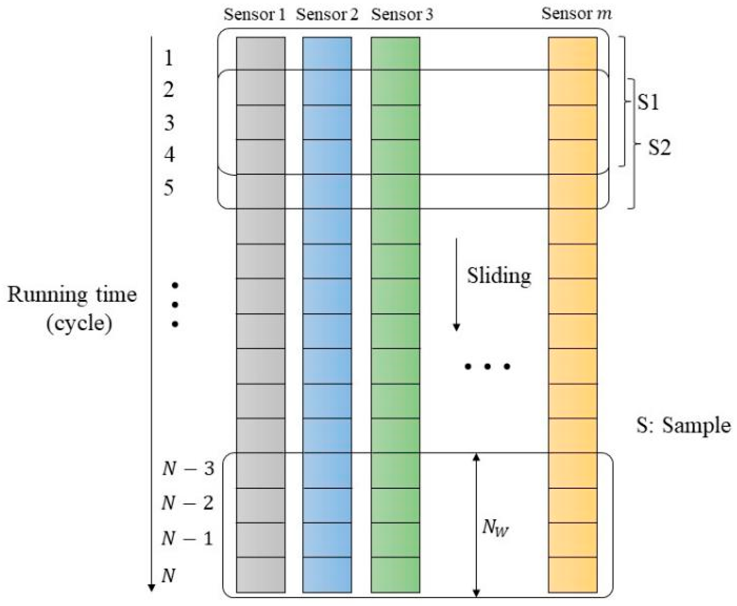
3.4. Data Preprocessing

Equation (16) is used for normalization [20] so that the data size is limited between $[0,1]$:

$${\tilde{x}}_i=\frac{x_i-x_i^{min}}{x_i^{max}-x_i^{min}},$$

(16)

where ${\tilde{x}}_i$ and $x_i$ are the normalized and original value, and $x_i^{min}$ and $x_i^{max}$ denote the minimum and maximum value of the $i$th sensor.

In the early stages of engine operation, due to the relative newness of the engine, it has a low failure rate, and the data change slowly. After that, the failure rate increases rapidly as the engine’s running time increases. Following previous work [24], a piecewise RUL labeling method was used, as shown in Figure 9. During the early stage of engine operation, RUL of the engine keeps a constant value, and then linearly decline until complete failure. Setting the initial RUL to 125 can achieve a better performance.

$${RUL}_{new}^i\left(t\right)=\left\{\begin{array}{l}125,\hspace{1em}\hspace{1em}t\le {RUL}^i-125\\ {RUL}^i-t,t>{RUL}^i-125\end{array},\right.$$

(17)

Each engine’s historical monitoring data are a time series, and because each engine’s running cycles are different, the lengths of these time series are not the same. To make each sample equal on the time scale, we use a sliding window to reconstruct the data, as shown in Figure 10. Suppose the historical data of an engine are $X={\left[X_1,X_2,\dots X_i,\dots X_N\right]}^T\in R^{N\times m}$, where $m$ is the number of monitored sensors and $N$ is the length of the time series. After the window sliding, we obtain the sample $S_i={\left[X_i,X_{i+1},\dots X_{i+N_w-1}\right]}^T$, where $N_w$ is the length of each sample in time dimension. After the sliding window, the historical data of one engine can be reconstructed into multiple samples containing the same time series length.

3.5. Network Parameter Configuration

The network parameters are set as shown in

Table 4. Parameters of the proposed model.

Hyperparameter	Value	Hyperparameter	Value
Window size	60	Activation in LSTM layer	tanh
Number of neurons in attention model	32	Number of LSTM layers	2
Kernel sizes for Conv1 to Conv3	7/12/17	Number of dense layers	1
Number of convolution kernels for Conv1 to Conv3	10/10/10	Dropout rate	0.1
Number of convolution layer	3	Activation in dense layer	linear
Padding	Same	Batch size	256
Activation in convolution layer	Relu	Loss function	MSE
Number of neurons in LSTM layer	100	Optimization function	Adam

. The sample size is (60,21), where each sample contains data from 21 sensors for 60 consecutive operating cycles. In the attention mechanism layer, there are 32 neurons used to calculate the similarity at different time steps. The multi-scale convolutional neural network layer employs 3 different kernel sizes: (7,1), (12,1), and (17,1). Each convolutional layer uses 10 of each type of kernel, and total of 3 convolutional layers are used. The model utilizes two LSTM layers, and to prevent overfitting, dropout mechanism is applied in the LSTM layer with a dropout rate of 0.1. Afterward, the model connects to a fully connected layer to predict RUL of the engine. The batch size is set as 256, the loss function is Mean Squared Error (MSE), and the optimization function is Adam.

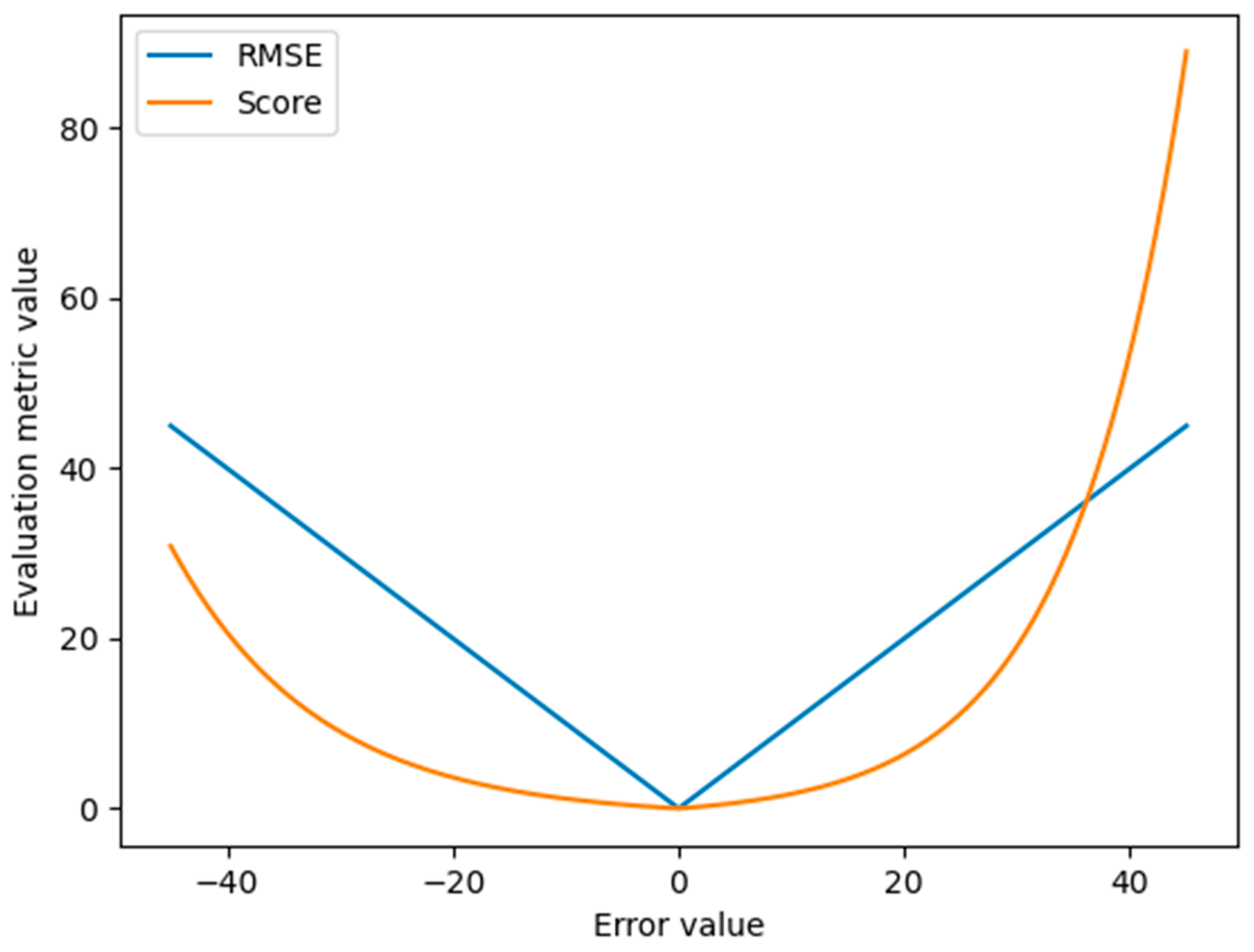
3.6. Evaluation Metrics

In order to evaluate the prediction accuracy of different methods, this paper uses three evaluation metrics that are widely used in the field of aircraft engine RUL prediction [14]. One is RMSE (Root Mean Square Error), another is Score, and the third is AS (Average Score). Their expressions are shown in Equations (18)–(20):

$$RMSE=\sqrt{\frac{1}{N}{\sum }_{i=1}^N\left({\hat{y}}_i-y_i\right)},$$

(18)

$$Score=\left\{\begin{array}{c}{\sum }_{i=1}^N\left(e^{-\frac{{\hat{y}}_i-y_i}{13}}-1\right),{\hat{y}}_i-y_i<0\\ {\sum }_{i=1}^N\left(e^{\frac{{\hat{y}}_i-y_i}{10}}-1\right),{\hat{y}}_i-y_i\ge 0\end{array}\right.,$$

(19)

$$AS=\frac{Score}{N},$$

(20)

where ${\hat{y}}_i$ denotes the predicted value of engine RUL, $y_i$ denotes the real value, and $N$ is the number of engines.

The $RMSE$ and $Score$ function graphs are shown in Figure 11, where the horizontal coordinates are the difference between ${\hat{y}}_i$ and $y_i$ (the prediction error), and the vertical coordinates are the function values. When the absolute value of the prediction error is equal, the value of the Score function with a prediction error greater than zero is larger than the value with a prediction error less than zero. An inaccurate prediction of RUL can have significant repercussions. For instance, if the predicted RUL is greater than the actual RUL, it may lead to premature engine maintenance, resulting in unnecessary costs and disruptions. On the other hand, if the predicted RUL is less than the actual RUL, it can result in delayed maintenance, increasing the risk of unexpected failures and potential safety hazards.

4. Experimental Results and Discussion

Experiments were carried out using a laptop computer with an AMD Ryzen 9 5900HX CPU and NVIDIA GeForce RTX 3080 Laptop GPU. In the conducted experiments, the software used was PyCharm 2022.2.3 (Community Edition), and the experiment code was based on Python 3.10.0 interpreter, Keras 2.8.0 API, and the Tensorflow 2.11.0 deep learning framework.

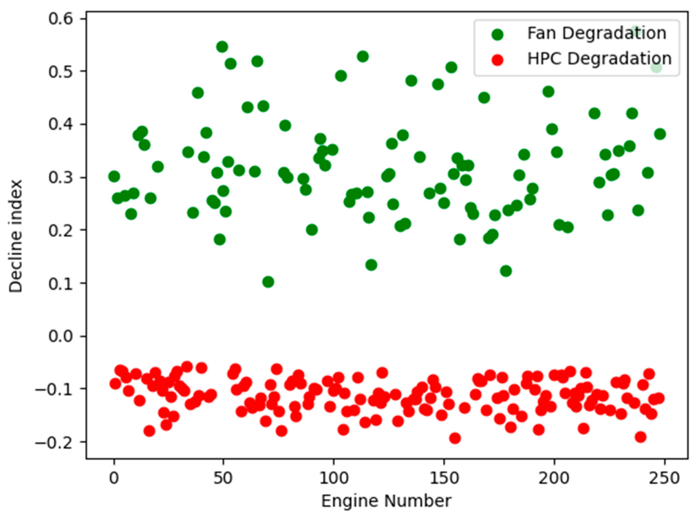
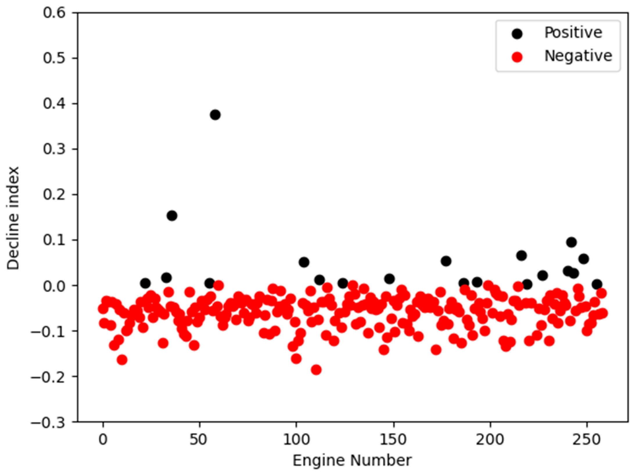
4.1. Fault Classification Results

Section 3.3 of this paper introduces the fault classification method. We utilize the metrics of P30, phi, and BPR for fault diagnosis. Considering their different magnitudes of deterioration, weightings of 1, 1, and −20 are assigned when calculating the decline index. The results of fault classification are shown in Figure 12, Figure 13 and Figure 14.

The x-axis represents the engine number, and the y-axis represents the decline index of the engine. Figure 12 is a scatter plot of the decline index values of all 260 engines in the FD002 training set. It is evident that all engines exhibit decline index values below 0. Figure 13 is a plot of the decline index values for all 249 engines in the FD004 training set. For the FD004 training set, engines with decline index values less than 0 are classified as experiencing HPC degradation faults, while engines with decline index values greater than 0 are classified as experiencing FAN degradation faults. Figure 13 clearly shows the distinct boundary between the two fault categories.

However, simply distinguishing the fault categories in the FD004 test set based on whether the decline index is greater than or less than 0 would result in a significant number of misclassifications. This is because the test set differs from the training set, and the test set contains a large number of engines that do not exhibit a clear degradation trend. These engines are significantly affected by noise in the slope fitting process, as shown in Figure 14. Figure 14 depicts the distribution of degradation indices in the FD002 test set, which only includes HPC degradation faults. Therefore, the majority of the decline index values in this distribution are below 0. However, due to noise disturbances, a small portion of engines without a clear degradation trend have decline index values greater than 0.

Hence, when classifying HPC faults in the FD004 test set, the threshold for the decline index is set to the 95th percentile of the decline index in the FD002 test set, which is −0.02.

The final HPC fault diagnostic results for the FD004 dataset are shown in

Table 5. Engine identification numbers diagnosed with HPC degradation fault.

Dataset	Engine Number
FD004 training dataset	2, 4, 5, 7, 8, 11, 13, 16, 17, 19, 20, 22, 23, 24, 25, 26, 27, 28, 29, 30, 31, 32, 33, 34, 36, 38, 40, 41, 44, 45, 55, 56, 57, 59, 60, 61, 63, 64, 67, 68, 70, 72, 73, 74, 75, 76, 77, 81, 82, 83, 84, 85, 86, 89, 90, 92, 93, 98, 99, 101, 102, 103, 105, 106, 107, 110, 112, 113, 115, 119, 120, 121, 122, 123, 124, 129, 130, 134, 135, 137, 138, 139, 141, 142, 143, 145, 146, 147, 150, 152, 153, 156, 160, 165, 166, 167, 168, 170, 172, 175, 176, 177, 178, 181, 182, 183, 186, 188, 189, 192, 193, 194, 195, 196, 197, 199, 201, 204, 205, 206, 208, 209, 210, 211, 212, 213, 214, 215, 216, 217, 218, 220, 222, 223, 226, 229, 231, 232, 233, 234, 237, 240, 241, 242, 244, 245, 246, 248
FD004 test dataset	2, 7, 8, 10, 14, 20, 22, 23, 26, 27, 31, 32, 35, 38, 42, 43, 47, 53, 58, 63, 67, 68, 69, 73, 77, 78, 80, 81, 82, 88, 90, 91, 92, 94, 96, 98, 101, 103, 106, 107, 113, 115, 116, 117, 120, 121, 124, 126, 131, 132, 136, 145, 147, 148, 150, 153, 154, 155, 156, 158, 159, 162, 163, 166, 167, 168, 169, 170, 172, 173, 174, 176, 177, 181, 182, 183, 184, 185, 187, 188, 196, 197, 198, 199, 200, 202, 204, 205, 208, 209, 210, 215, 216, 217, 218, 219, 224, 225, 226, 229, 230, 233, 234, 237, 238, 239, 241, 242, 244, 247, 248

. In the FD004 training set, a total of 148 engines were diagnosed with HPC degradation faults, while in the FD004 test set, a total of 111 engines were diagnosed with HPC degradation faults.

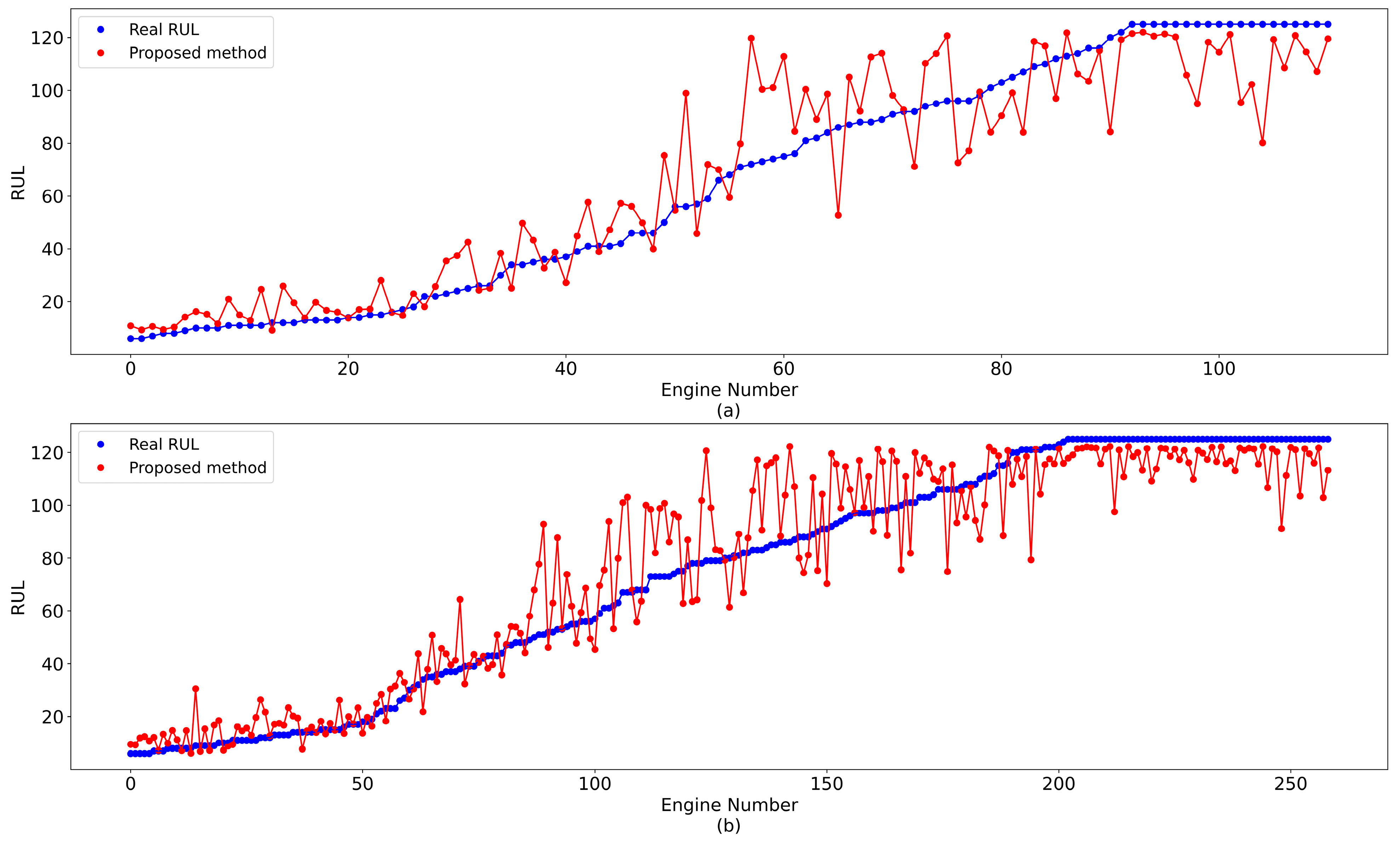
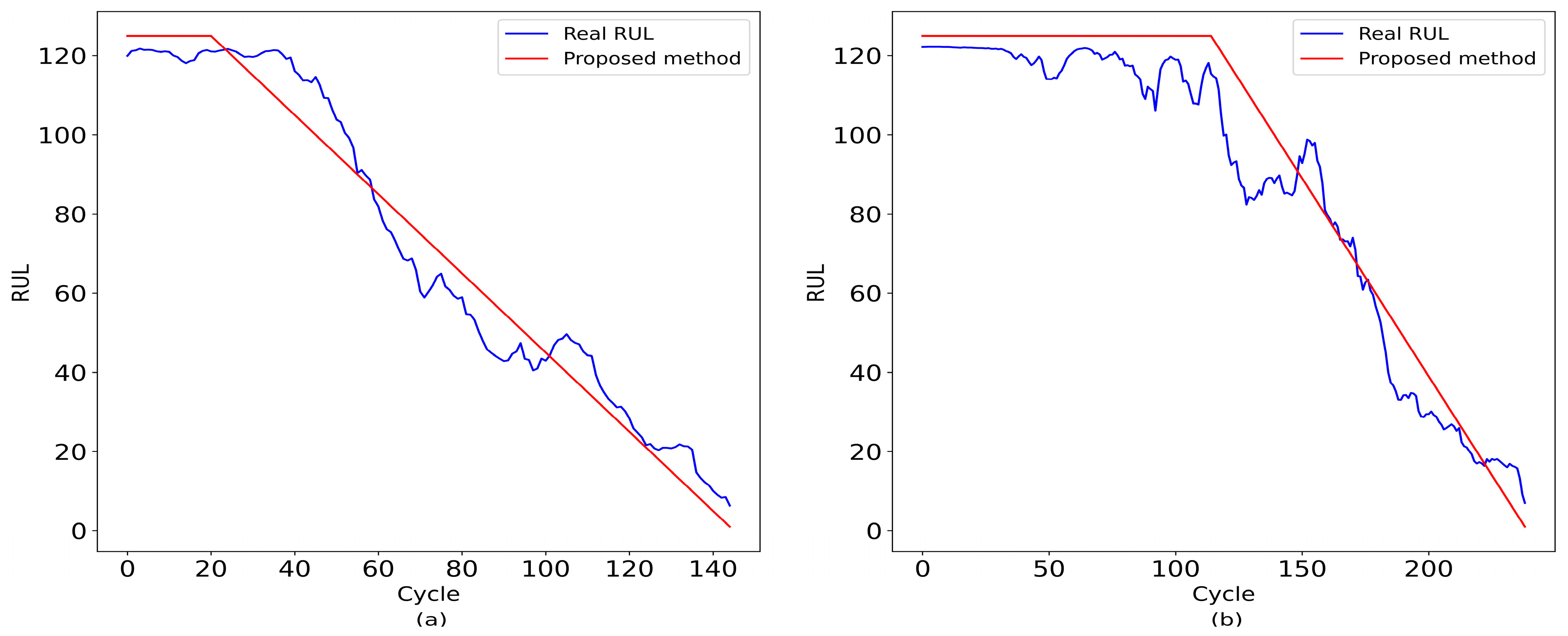
4.2. Prediction Results and Degradation Experiments

During the model training process, the 148 engines diagnosed with HPC degradation faults from both the FD002 training set and FD004 training set were combined as the training dataset to predict the engines in the FD002 test set and the engines diagnosed with HPC degradation faults in the FD004 test set. The prediction results are shown in Figure 15. The x-axis represents the engine number, where the engine numbers have been re-ordered based on the true RUL values of the engines. The y-axis represents RUL values, where the blue dots represent the true values and the red dots represent the predicted values.

By examining Figure 15, it becomes apparent that the model achieves high prediction accuracy during normal engine operation at the initial stages and near the point of failure. However, during the middle stage of degradation, the prediction errors are higher. This phenomenon arises due to the distinct pattern of sensor data decline observed as the engine approaches failure. However, during the intermediate stage of engine degradation, the sensor data do not show significant changes and are susceptible to noise, leading to larger errors in predictions.

A random engine was selected from both the FD002 training set and the FD004 training set to observe its fitting performance, and the results are shown in Figure 16. The x-axis represents the engine operating cycles, and the y-axis represents the engine RUL values. The model demonstrates a strong overall fitting performance, as evidenced by the results. However, due to the presence of system noise, there is still a significant gap between the predicted values and the true values during the middle stage of degradation.

To compare the effectiveness of the fault classification method,

Table 6. Performance with respect to different training datasets.

Training Dataset	FD002 Test Dataset		FD004 Test Dataset (HPC Degradation)
	RMSE	Score	RMSE	Score
FD002 training dataset + FD004 training dataset (HPC degradation)	13.59	893.55	15.25	520.00
FD002 training dataset + FD004 training dataset	16.44	2721.62	17.54	2221.76
FD002 training dataset	14.29	1003.13	-	-
FD004 training dataset	-	-	19.48	935.42

presents a comparison of the prediction errors on the test sets under different training data scenarios. For the FD002 test set, three training datasets were used, including the traditional approach of training only on the FD002 training set, training on the combined FD002 training set and all FD004 training sets, and training on the FD002 training set and only the engines with HPC degradation faults from the FD004 training set. Similarly, for the FD004 test set (HPC degradation), three training datasets were used, including training only on the FD004 training set, training on the combined FD002 training set and all FD004 training sets, and training on the FD002 training set and only the engines with HPC degradation faults from the FD004 training set.

The results demonstrate that compared to the traditional approach of using a single training dataset to predict the corresponding test set engine RUL, the proposed method significantly improves the prediction accuracy when the engine experiences HPC faults. The RMSE and Score values for the FD002 test set are reduced by 4.9% and 10.9%, respectively. For the FD004 test set, the RMSE and Score values are reduced by 21.7% and 44.4%, respectively. Furthermore, blindly incorporating engine data with different fault patterns can even decrease the prediction accuracy of the model. For instance, when training on the combined FD002 dataset and all FD004 engines, the Score values for the FD002 test set and FD004 test set increased by 171.5% and 137.5%, respectively.

Overall, these findings highlight the improved prediction accuracy of the proposed method compared to the traditional approach, particularly for engines experiencing HPC faults. Additionally, caution is necessary when introducing engine data with different fault patterns into the training process to prevent potential degradation in prediction performance.

The error distribution histograms for the three training datasets are shown in Figure 17. The histogram is used to display the distribution of the prediction errors for RUL. RUL prediction error is obtained by subtracting the predicted RUL value from the true RUL value. To showcase the distribution of this error, the errors are divided into several equally sized intervals, and the number of engines falling into each interval is counted.

The x-axis of Figure 17 likely represents the range or intervals of the errors, while the y-axis represents the number of engines in each interval (frequency). By using the histogram, the distribution of RUL prediction errors can be observed, including measures of central tendency, outliers, and other relevant information.

Figure 17a–c represent the error distributions for the FD002 test set using the FD002 training dataset and FD004 training dataset (HPC degradation), the FD002 training dataset and FD004 training dataset, and the FD002 training dataset, respectively. Figure 17d–f represent the error distributions for the FD004 test set using the FD002 training dataset and FD004 training dataset (HPC degradation), the FD002 training dataset and FD004 training dataset, and the FD004 training dataset, respectively. The x-axis represents the difference between the predicted values and the actual values, while the y-axis represents the frequency.

Figure 17 reveals that when utilizing the combined FD002 dataset and all FD004 training datasets, the interference among different fault patterns results in notable deviations in RUL predictions for certain engines. Compared to the traditional approach of training the model using a single dataset to predict the RUL of the test set engines, the proposed method results in a more concentrated error distribution around zero for the FD002 test set due to the increased training dataset. For the FD004 test set, the proposed method eliminates the interference between different faults through the fault classification method, resulting in a significant improvement in prediction accuracy.

Overall, these findings suggest that the proposed method achieves enhanced prediction accuracy for the FD002 test set due to the increased training dataset, and for the FD004 test set, the proposed method effectively improves prediction accuracy by eliminating interference between different fault patterns.

Table 7. Performance with respect to different decline index thresholds.

Threshold	FD004 Test Dataset (HPC Degradation)
	RMSE	Score	Total Engine Number	AS
−0.02	15.25	520.00	111	4.68
−0.03	14.64	406.52	99	4.11
−0.04	13.33	308.10	83	3.71
−0.05	12.70	268.21	72	3.73
−0.06	12.13	223.21	62	3.60

shows the impact of different decline index thresholds on the prediction results. It is apparent that as the absolute value of the decline index threshold increases, indicating a more stringent diagnosis of HPC (High-Pressure Compressor) faults, the number of engines classified as having HPC faults decreases. However, this reduction in the number of engines is accompanied by a notable improvement in accuracy.

As the threshold decreases from −0.02 to −0.06, the RMSE value for the FD004 test set used in this study decreases by 20%. As the absolute value of the decline index threshold increases, the degradation trend of engines classified as HPC faults becomes more pronounced. Consequently, engines with a clear degradation trend exhibit higher prediction accuracy. However, in terms of the average score of the engines, the improvement in accuracy from the threshold decreasing from −0.02 to −0.04 is much greater than the improvement from the threshold decreasing from −0.04 to −0.06. This indicates that there is a risk of misclassification when the absolute value of the decline index threshold is low, leading to a significant decrease in AS when the threshold starts to decrease.

Overall, these findings suggest that increasing the absolute value of the decline index threshold improves prediction accuracy, especially for engines with a clear degradation trend. However, there is a trade-off between accuracy and the risk of misclassification, as lower threshold values carry a higher risk of misclassification, resulting in a significant decrease in AS.

In this experiment, we investigated the impact of varying the number of neurons in the attention layer on the prediction performance while keeping the other parameters of the network constant.

Table 8. Model evaluation metrics under different attention mechanism layer neuron counts.

Number	FD002 Test Dataset		FD004 Test Dataset (HPC Degradation)
	RMSE	Score	RMSE	Score
16	15.64	1045.75	16.88	704.64
32	13.59	893.55	15.25	520.00
64	14.55	963.13	16.33	645.53

presents the results, displaying the corresponding prediction metric values for different numbers of neurons—specifically 16, 32, and 64. These results provide insights into how the performance of the model is affected by the choice of neuron count in the attention layer.

Based on the observations from Table 8, it is evident that the prediction performance is influenced by the number of neurons in the attention layer. However, it is crucial to note that increasing the number of neurons enhances the model’s capacity to fit the data, but an excessive number of neurons can lead to the problem of overfitting. Overfitting occurs when the model performs well on the training set but fails to generalize on the test set. Considering the comprehensive experimental results depicted in Table 8, a careful decision has been made to select 32 neurons as the optimal parameter setting for the network. This choice strikes a balance between the model’s fitting ability and the risk of overfitting, ensuring reliable performance without compromising computational efficiency.

Each MSCNN and LSTM layer possesses the capability to extract features at different dimensions. By stacking multiple MSCNN or LSTM layers, higher-level features can be systematically extracted, thereby enhancing the model’s feature representation capabilities. However, increasing the number of layers results in increased model complexity and a higher risk of overfitting.

In the experiment, we systematically increased the number of MSCNN layers from 1 to 4 and LSTM layers from 1 to 3. The corresponding performance metrics, RMSE and Score, are detailed in

Table 9. Model evaluation metrics under different MSCNN layers.

Number	Total Parameters	FD002 Test Dataset		FD004 Test Dataset (HPC Degradation)
		RMSE	Score	RMSE	Score
1	141,900	15.14	1046.23	17.23	721.54
2	152,730	14.28	983.45	16.68	680.77
3	163,560	13.59	893.55	15.25	520.00
4	174,390	13.76	920.43	15.78	542.61

and

Table 10. Model evaluation metrics under different LSTM layers.

Number	Total Parameters	FD002 Test Dataset		FD004 Test Dataset (HPC Degradation)
		RMSE	Score	RMSE	Score
1	83,160	15.22	1123.21	16.85	702.59
2	163,560	13.59	893.55	15.25	520.00
3	243,960	14.55	1022.14	16.22	611.23

. These experimental results provide insights into the impact of layer count on the model’s performance.

In Table 9, it is evident that the feature-extraction capabilities of the proposed model exhibit an initial improvement followed by a decline as the number of MSCNN layers increases. When the MSCNN layer count exceeds 3, the model’s performance starts to deteriorate. Based on these findings, the optimal choice is to select three layers for the MSCNN architecture.

Similarly, Table 10 presents prediction results similar to those in Table 9. LSTM is well-suited for handling problems closely related to time series. However, adding additional LSTM layers introduces a large number of parameters, which can weaken the model’s generalization ability. According to Table 10, the optimal choice is to select two layers for the LSTM architecture.

Table 11. Performance comparisons of different methods.

Method	FD002 Test Dataset			FD004 Test Dataset (HPC Degradation)
	RMSE	Score	AS	RMSE	AS
LSTM [29] (2017)	24.49	4450	17.87	28.17	22.38
Transformer + TCNN [30] (2021)	15.35	1267	5.09	18.35	8.55
Spatio-temporal GCN [31] (2021)	17.74	2485.02	9.98	18.08	10.38
DAST [32] (2022)	15.25	924.96	3.71	18.36	6.01
BiGRU-TSAM [33] (2022)	18.94	2264.13	9.09	20.47	14.56
Double attention-based architecture [15] (2022)	17.08	1575	6.33	19.86	7.02
Transformer Encoder + Attention [34] (2023)	15.82	1008.08	3.89	17.35	7.06
MSDCNN [24] (2023)	18.70	1873.86	7.53	21.57	10.88
Proposed method	13.59	893.55	3.59	15.25	4.68

presents the accuracy comparison results of the proposed method with other methods. Since the C-MAPSS dataset is a publicly available dataset, all the methods listed in Table 11 use the same data. The accuracy data for these methods are sourced from their respective original publications.

The table clearly indicates that LSTM networks exhibit the lowest prediction accuracy in the FD002 and FD004 test sets, primarily due to their limited feature-extraction capabilities. In order to enhance the feature-extraction ability of the model in complex data, researchers have proposed many new network models. For example, transformers with the TCNN model, DAST, and Double Attention-based Architecture have used transformers to handle the temporal similarity of sequential data. In order to address the lack of powerful spatiotemporal learning ability in traditional CNN networks, variants of CNN networks such as MSDCNN and GCN have also been used for engine RUL prediction. However, these methods fail to address the interference between different fault modes in RUL fitting, leading to a significant decrease in accuracy when predicting the FD004 dataset.

Compared to these methods, the approach in this paper increases the training data of 148 engines in the FD002 test set. This results in a 10.9% improvement in RMSE value and a 3.4% improvement in Score value. For the FD004 test set, although this paper only predicts 111 engines, the errors in RMSE and AS show a reduction of 15.7% and 22.1%, respectively. The improvement in accuracy for the FD004 dataset is greater than that of the FD002 test dataset. This is because fault classification is used to eliminate the influence of fan degradation fault data on HPC degradation fault data, and then 250 engine data from the FD002 training set are added for training. This significantly improves the accuracy of the approach in targeting the FD004 dataset (HPC degradation).

5. Conclusions

This paper addresses the challenge of coupling multiple operating conditions and multiple fault modes in predicting the RUL of aircraft engines. To tackle this issue, we propose a decay index to classify the degradation faults of the HPC and fan, followed by the development of an AMSLSTM network specifically for HPC fault prediction and RUL estimation. By categorizing faults, our method transforms the problem of RUL prediction under multiple fault modes into a single fault mode scenario. The experiments conducted on the C-MAPSSS dataset demonstrate that our approach significantly improves the accuracy of RUL prediction for HPC degradation faults under various operating conditions compared to other methods. We validate the effectiveness of fault classification through predictions using different training datasets and analyze the impact of different decay index thresholds on the prediction results.

In existing studies, the RUL of aircraft engines is often modeled as piecewise functions, exhibiting initial constancy followed by linear degradation. However, in real-world aircraft engine lifetimes, maintenance is a significant factor that can impact RUL values. Maintenance activities have the potential to enhance engine reliability and performance, thereby extending their useful life. In future work, we plan to analyze the timing of maintenance events and their effect on the RUL of aircraft engines.

References

1. Kamran, J.; Rafael, G.; Noureddine, Z. State of the art and taxonomy of prognostics approaches, trends of prognostics applications and open issues towards maturity at different technology readiness levels. Mech. Syst. Signal Process. 2017, 94, 214–236. [Google Scholar]
2. Zhao, Z.; Liang, B.; Wang, X.; Lu, W. Remaining useful life prediction of aircraft engine based on degradation pattern learning. Reliab. Eng. Syst. Saf. 2017, 164, 74–83. [Google Scholar] [CrossRef]
3. Lee, J.; Wu, F.; Zhao, W.; Ghaffari, M.; Liao, L.; Siegel, D. Prognostics and health management design for rotary machinery systems-reviews, methodology and applications. Mech. Syst. Signal Process. 2014, 42, 314–334. [Google Scholar] [CrossRef]
4. Bolander, N.; Qiu, H.; Eklund, N.; Hindle, E.; Rosenfeld, T. Physics-based remaining useful life prediction for aircraft engine bearing prognosis. In Proceedings of the Annual Conference of the PHM Society, San Diego, CA, USA, 27 September–1 October 2009. [Google Scholar]
5. Matthew, J.D.; Goebel, K. Model-Based Prognostics with Concurrent Damage Progression Processes. IEEE Trans. Syst. Man Cybern. 2013, 43, 535–546. [Google Scholar]
6. Jaouher, B.A.; Brigitte, C.; Lotfi, S.; Simon, M.; Farhat, F. Accurate bearing remaining useful life prediction based on Weibull distribution and artificial neural network. Mech. Syst. Signal Process. 2015, 56, 150–172. [Google Scholar]
7. Yu, W.; Tu, W.; Kim, I.; Mechefske, C. A nonlinear-drift-driven Wiener process model for remaining useful life estimation considering three sources of variability. Reliab. Eng. Syst. Saf. 2021, 212, 107631. [Google Scholar] [CrossRef]
8. Yan, J.; Lee, J. Degradation Assessment and Fault Modes Classification Using Logistic Regression. J. Manuf. Sci. Eng. 2005, 127, 912–914. [Google Scholar] [CrossRef]
9. Chen, Z.; Li, Y.; Xia, T.; Pan, E. Hidden Markov model with auto-correlated observations for remaining useful life prediction and optimal maintenance policy. Reliab. Eng. Syst. Saf. 2019, 184, 123–136. [Google Scholar] [CrossRef]
10. Li, X.; Wu, S.; Li, X.; Yuan, H.; Zhao, D. Particle swarm optimization-support vector machine model for machinery fault diagnoses in high-voltage circuit breakers. Chin. J. Mech. Eng. 2020, 33, 104–113. [Google Scholar] [CrossRef]
11. Babu, G.S.; Zhao, P.; Li, X.L. Deep Convolutional Neural Network Based Regression Approach for Estimation of Remaining Useful Life. In Database Systems for Advanced Applications Navathe; Navathe, S., Wu, W., Shekhar, S., Du, X., Wang, X., Xiong, H., Eds.; Springer: Cham, Switzerland, 2016; pp. 214–228. [Google Scholar]
12. Hochreiter, S.; Schmidhuber, J. Long short-term memory. Neural Comput. 1997, 9, 1735–1780. [Google Scholar] [CrossRef] [PubMed]
13. Kong, Z.; Cui, Y.; Xia, Z.; Lv, H. Convolution and long short-term memory hybrid deep neural networks for remaining useful life prognostics. Appl. Sci. 2009, 9, 4156. [Google Scholar] [CrossRef]
14. Boujamza, A.; Elhaq, S. Attention-based LSTM for Remaining Useful Life Estimation of Aircraft Engines. IFAC PapersOnLine 2022, 55, 450–455. [Google Scholar] [CrossRef]
15. Liu, L.; Song, X.; Zhou, Z. Aircraft engine remaining useful life estimation via a double attention-based data-driven architecture. Reliab. Eng. Syst. Saf. 2022, 221, 108330. [Google Scholar] [CrossRef]
16. Khumprom, P.; Grewell, D.; Yodo, N. Deep Neural Network Feature Selection Approaches for Data-Driven Prognostic Model of Aircraft Engines. Aerospace 2020, 7, 132. [Google Scholar] [CrossRef]
17. Zhang, Y.; Feng, K.; Ji, J.C.; Yu, K.; Ren, Z.; Liu, Z. Dynamic Model-Assisted Bearing Remaining Useful Life Prediction Using the Cross-Domain Transformer Network. IEEE/ASME Trans. Mechatron. 2023, 28, 1070–1080. [Google Scholar] [CrossRef]
18. Zhang, Y.; Yu, K.; Lei, Z.; Ge, J.; Xu, Y.; Li, Z.; Ren, Z.; Feng, K. Integrated intelligent fault diagnosis approach of offshore wind turbine bearing based on information stream fusion and semi-supervised learning. Expert Syst. Appl. 2023, 232, 120854. [Google Scholar] [CrossRef]
19. Xiang, F.; Zhang, Y.; Zhang, S.; Wang, Z.; Qiu, L.; Choi, J.H. Bayesian gated-transformer model for risk-aware prediction of aero-engine remaining useful life. Expert Syst. Appl. 2024, 238, 121859. [Google Scholar] [CrossRef]
20. Zhang, X.; Sun, J.; Wang, j.; Jin, Y.; Wang, L.; Liu, Z. PAOLTransformer: Pruning-adaptive optimal lightweight Transformer model for aero-engine remaining useful life prediction. Reliab. Eng. Syst. Saf. 2023, 240, 109605. [Google Scholar] [CrossRef]
21. Chen, Z.; Wu, M.; Zhao, R.; Guretno, F.; Yan, R.; Li, X. Machine Remaining Useful Life Prediction via an Attention-Based Deep Learning Approach. IEEE Trans. Ind. Electron. 2021, 68, 2521–2531. [Google Scholar] [CrossRef]
22. Zhang, H.; Zhang, Q.; Shao, S.; Niu, T.; Yang, X. Attention-Based LSTM Network for Rotatory Machine Remaining Useful Life Prediction. IEEE Access 2020, 8, 132188–132199. [Google Scholar] [CrossRef]
23. Ren, L.; Dong, J.; Wang, X.; Meng, Z.; Zhao, L.; Deen, M.J. A Data-Driven Auto-CNN-LSTM Prediction Model for Lithium-Ion Battery Remaining Useful Life. IEEE Trans. Ind. Inform. 2021, 17, 3478. [Google Scholar] [CrossRef]
24. Chen, W.; Liu, C.; Chen, Q.; Wu, P. Multi-scale memory-enhanced method for predicting the remaining useful life of aircraft engines. Neural Comput. Appl. 2023, 35, 2225–2241. [Google Scholar] [CrossRef]
25. Meng, M.; Mao, Z. Deep-Convolution-Based LSTM Network for Remaining Useful Life Prediction. IEEE Trans. Ind. Inform. 2021, 17, 1658–1667. [Google Scholar]
26. Saxena, A.; Goebel, K.; Simon, D.; Eklund, N. Damage Propagation Modeling for Aircraft Engine Run-to-Failure Simulation. In Proceedings of the International Conference on Prognostics and Health Management (PHM), Denver, CO, USA, 6–9 October 2008; pp. 1–9. [Google Scholar]
27. Saxena, A.; Goebel, K. Turbofan Engine Degradation Simulation Data Set; NASA Ames Prognostics Data Repository; NASA Ames: Moffett Field, CA, USA, 2008.
28. Luo, M. Data-Driven Fault Detection Using Trending Analysis. Doctoral Dissertation, Louisiana State University and Agricultural and Mechanical College, Baton Rouge, LA, USA, 2006. [Google Scholar]
29. Zheng, S.; Ristovski, K.; Farahat, A.; Gupta, C. Long Short-Term Memory Network for Remaining Useful Life estimation. In Proceedings of the 2017 IEEE International Conference on Prognostics and Health Management (ICPHM), Dallas, TX, USA, 19–21 June 2017; pp. 88–95. [Google Scholar]
30. Wang, H.; Cheng, Y.; Song, K. Remaining useful life estimation of aircraft engines using a joint deep learning model based on TCNN and transformer. Comput. Intell. Neurosci. 2021, 2021, 5185938. [Google Scholar] [CrossRef] [PubMed]
31. Wang, M.; Li, Y.; Zhang, Y.; Jia, L. Spatio-temporal graph convolutional neural network for remaining useful life estimation of aircraft engines. Aerosp. Syst. 2021, 4, 29–36. [Google Scholar] [CrossRef]
32. Zhang, Z.; Song, W.; Li, Q. Dual-aspect self-attention based on transformer for remaining useful life prediction. IEEE Trans. Instrum. Meas. 2022, 71, 1–11. [Google Scholar] [CrossRef]
33. Zhang, J.; Jiang, Y.; Wu, S.; Li, X.; Luo, H.; Yin, S. Prediction of remaining useful life based on bidirectional gated recurrent unit with temporal self-attention mechanism. Reliab. Eng. Syst. Saf. 2022, 221, 108297. [Google Scholar] [CrossRef]
34. Wang, X.; Li, Y.; Xu, Y.; Liu, X.; Zheng, T.; Zheng, B. Remaining Useful Life Prediction for Aero-Engines Using a Time-Enhanced Multi-Head Self-Attention Model. Aerospace 2023, 10, 80. [Google Scholar] [CrossRef]
Figure 1. Structure of attention mechanism.
Aerospace 11 00293 g001
Figure 2. Structure of the MSCNN model.
Aerospace 11 00293 g002
Figure 3. Structure of the LSTM model.
Aerospace 11 00293 g003
Figure 4. Architecture of the proposed AMSLSTM model.
Aerospace 11 00293 g004
Figure 5. Proposed framework for RUL predictions.
Aerospace 11 00293 g005
Figure 6. Comparison of P30 data of an engine before and after classification of operating conditions. (a) are the original data, and (bg) is the distribution of data in operating conditions 1~6 after classification.
Aerospace 11 00293 g006
Figure 7. BPR data graph for all engines in the FD002 training dataset under operating condition 1.
Aerospace 11 00293 g007
Figure 8. BPR data graph for all engines in the FD004 training dataset under operating condition 1.
Aerospace 11 00293 g008
Figure 9. Piecewise RUL labeling.
Aerospace 11 00293 g009
Figure 10. Sliding window processing.
Aerospace 11 00293 g010
Figure 11. Graph of RMSE and Score function.
Aerospace 11 00293 g011
Figure 12. Decline index value of engines in FD002 training dataset.
Aerospace 11 00293 g012
Figure 13. Decline index value of engines in FD004 training dataset.
Aerospace 11 00293 g013
Figure 14. Decline index value of engines in FD002 test dataset.
Aerospace 11 00293 g014
Figure 15. RUL prediction results of test dataset: (a) FD004 (HPC degradation) test dataset, and (b) FD002 test dataset.
Aerospace 11 00293 g015
Figure 16. RUL prediction results. (a) shows an engine in FD002, and (b) shows an engine in FD004.
Aerospace 11 00293 g016
Figure 17. Error distribution histogram. (ac) are FD002 test dataset results. (df) are FD004 test dataset (HPC degradation) results. (a,d) use FD002 training dataset and FD004 training dataset (HPC degradation). (b,e) use FD002 training dataset and FD004 training dataset. (c) uses FD002 training dataset. (f) uses FD004 training dataset.
Aerospace 11 00293 g017