Artificial Intelligence Approach in Aerospace for Error Mitigation

Abstract

Many of the reports created at assembly lines, where all components of an aircraft are installed, frequently indicate that errors threaten safety. The proposed methodology in this study evaluates error prediction and risk mitigation to prevent failures and their consequences. The results linked to a typical electrical harness manufacture of a military aircraft estimated reductions of 93% in time and 90% in error during the creation of engineering manufacturing processes using AI techniques. However, traditional risk assessments methods struggle to identify and mitigate errors effectively. Thus, developing an advanced methodology to ensure systems safety is needed. This paper addresses how innovative AI technology solutions can overcome these challenges, mitigate error risks, and enhance safety in aerospace. Technologies, such as artificial intelligence, predictive algorithms, machine learning, and automation, can play a key role in enhancing safety. The aim of this study is to develop a model that considers the factors that can potentially contribute to error creation, through an artificial intelligence (AI) approach. The specific AI techniques used such as support vector machine, random forest, logistic regression, K-nearest neighbor, and XGBoost (Python 3.8.5) show good performance for use in error mitigation. We have compared the modeled values obtained in this study with the experimental ones. The results confirm that the best metrics are obtained by using support vector machine and logistic regression. The smallest deviation between the measured and modeled values for these AI methods do not exceed 5%. Furthermore, using advancements in machine learning methods can enhance error mitigation in aerospace. The use of AutoML can play a key role in automatically finding an appropriate model which provides the best performance metrics and therefore the most reliable forecast for data prediction and error mitigation.

1. Introduction

In the aerospace safety field, there are different types of data collected to analyze accidents, non-conformances, deviations, and errors. Safety databases are composed of reports with integrated tools to allow the creation of understandable data for analysts in different formats. Typically, systems for quality, security, and safety are integrated into the aerospace organization and monitored to ensure compliance with safety standards like International Civil Aviation Organization (ICAO) Annex 19 [1]. Traditional methods use indicators to define an event as being acceptable. Most of the investigation processes, which are related to the identification of these factors, aim to evaluate undesired outcomes [2]. Risk assessment processes are fundamental to identify, evaluate, and mitigate potential risks. The approach of risk mitigation by assessment is considered critical to safe operations [3]. Aviation has developed aeronautical decision-making systems, which consider factors such as requirements, aircraft performance, and safety parameters to help make the best decisions [4]. A risk matrix is used to evaluate the likelihood and consequences of an event. After defining the risk, impact mitigation techniques are applied to avoid potential errors [5,6]. However, the limitations of current databases in safety risk assessment prevent the provision of efficient risk mitigation measures. Therefore, ensuring safety at the highest level is compromised.

Aerospace safety risk refers to the evaluation of undesired situations that may lead to accidents or incidents. Undesired outcomes and hazards may be present in all aerospace activities. There are associated uncertainties that need to be properly considered in order to avoid higher risks [7]. Thus, continuous safety monitoring is performed to manage these undesired factors. Events such as equipment damage, serious incidents, injury to people, or multiple deaths may occur. Measures for risk mitigation are directly associated with safety risk [8]. The methods used to control safety risks rely on likelihood analysis of safety outcomes, considering factors such as equipment failures or human errors. Strategies to mitigate these risks are also established for this purpose [9].

Aerospace activities result from a chain of complex events involving multiple variables and different scenarios with rapid changes that require fast decisions. The multiple dependent variables involved in the end-to-end process make aerospace activities susceptible to hazards. In particular, aerospace is affected by latent conditions such as design and manufacturer decisions, procedure writers, management, and maintenance activities [10]. These conditions are generated mainly by people who make incorrect decisions within inadequate organizational processes. Consequently, real-time hazard predictions are a cutting-edge approach to challenge. Continuous research and development in aviation technology aim to enhance safety methods, making them more effective in anticipating and preventing failures [11].

In recent years, data have grown exponentially; therefore, requirements are more difficult to meet and errors may appear more often. Electrical systems are more complex and higher data accuracy is required for efficient performance [12]. New technology has improved flight safety. However, there is evidence that human errors are the main trigger for errors [13,14]. Systems have increased in complexity and more interconnections are necessary for good performance [7]. The complexity and interconnection of aerospace systems can contribute to increasing the probability of error creation and failure propagation. Current approaches do not have the necessary capability to address potential risk and to establish strategies for error mitigation. Thus, the integration of advanced error mitigation using AI methods to evaluate the risk of error creation under real-time conditions is necessary. AI approaches can provide innovative solutions to overcome the limitations of existing techniques.

Concerning safety issues, different approaches, such as manufacturing processes based on the latest 4.0 technology, are solutions to produce final safety products [15]. Industry 4.0 is based on a methodology that represents a smart chained network where machines and products interact with each other automatically. This technology can not only improve flight safety [16], but also has a significant impact on overcoming challenges and enhancing sustainable business performance.

The safety process involves identification problems that appear in the early design stage through an approach aiming to identify future threats by prediction. The use of AI techniques provides more evidence for more accurate decision making [17,18]. Predictive algorithms developed in this context with application to aerospace can play a key role in preventing failures [19] and consequently in preventing accidents and saving human lives.

Artificial intelligence technology can prevent undesired situations from occurring [20]. The integration of AI into design models has the potential to enhance safety and reliability. AI models can not only handle complex and nonlinear data but also have the capacity to anticipate errors and make the best decisions in case uncertainties appear. Furthermore, advanced analytics and AI algorithm development can analyze large amounts of data to identify patterns which can potentially contribute to create failures [21]. All of these factors are relevant for use as references for safety in aviation [22].

This innovative approach leverages a risk matrix function, which enables a structured evaluation and visualization of threats. This approach is driven by real-time data, which require a dynamic understanding of risk by considering multiple factors and probabilistic approaches for making real-time decisions [23]. The methodology established in this study will accelerate the development of tasks, monitor real-time data, and assess the risk of error creation and its severity. Using the algorithm’s insights, the best decision can be made in the dynamic manufacturing area and in simultaneously forecasting the risk of error creation for new datasets [24,25,26].

The main aim of this study is to prevent failures in existing manufacturing processes by applying techniques based on AI machine learning. Moreover, this methodology enhances efficiency and productivity by integrating this technology in the engineering processes and enabling real-time communication between interconnected devices [17,27,28]. The use of automation of existing manual tasks will not only improve the work delivered from the engineering to the manufacturing area, but will also reduce the human decision factor, thereby decreasing the risk of accidents. Vulnerabilities may compromise the data, increasing the risks of cyberattacks. Consequently, security strategies are implemented to protect the integrity of the algorithm [29].

The objectives of this research are to design an AI model to mitigate errors and evaluate their risks in the aerospace manufacturing assembly line. In particular, support vector machine (SVM), random forest (RF), logistic regression (LR), K-nearest neighbor (KNN), and XGBoost (eXtreme Gradient Boosting) have been used and evaluated using the following metrics: accuracy, precision, recall, and F₁-score. Additionally, this approach can not only reduce errors but potentially enhance efficiency and bring improvements in the aerospace manufacturing assembly line. Overall, this study aims to enhance safety and keep aerospace at the highest level [30].

2. Materials and Methods

Aerospace frequently uses a high volume of electrical harness drawings. Three-dimensional models are used to create a full-scale drawing enriched with manufacturing information, which is called a Formboard drawing. Harness assessment is performed using a computer-aided-design (CAD) model that represents an assembly with electrical components. The risk matrix is calculated according to the criteria shown in Table 1, which is based on the following input parameters: number of wires (H), terminations (Z), and electrical components (N). The most vulnerable stage, in terms of error creation, involves harness transformation from the current model to a flattened model. Electrical parameters are added to the model in order to flatten the 3D model accordingly. The generated mesh is extracted using an automatic script. The target is to flatten the entire mesh generated in the real length to produce a 2D model.

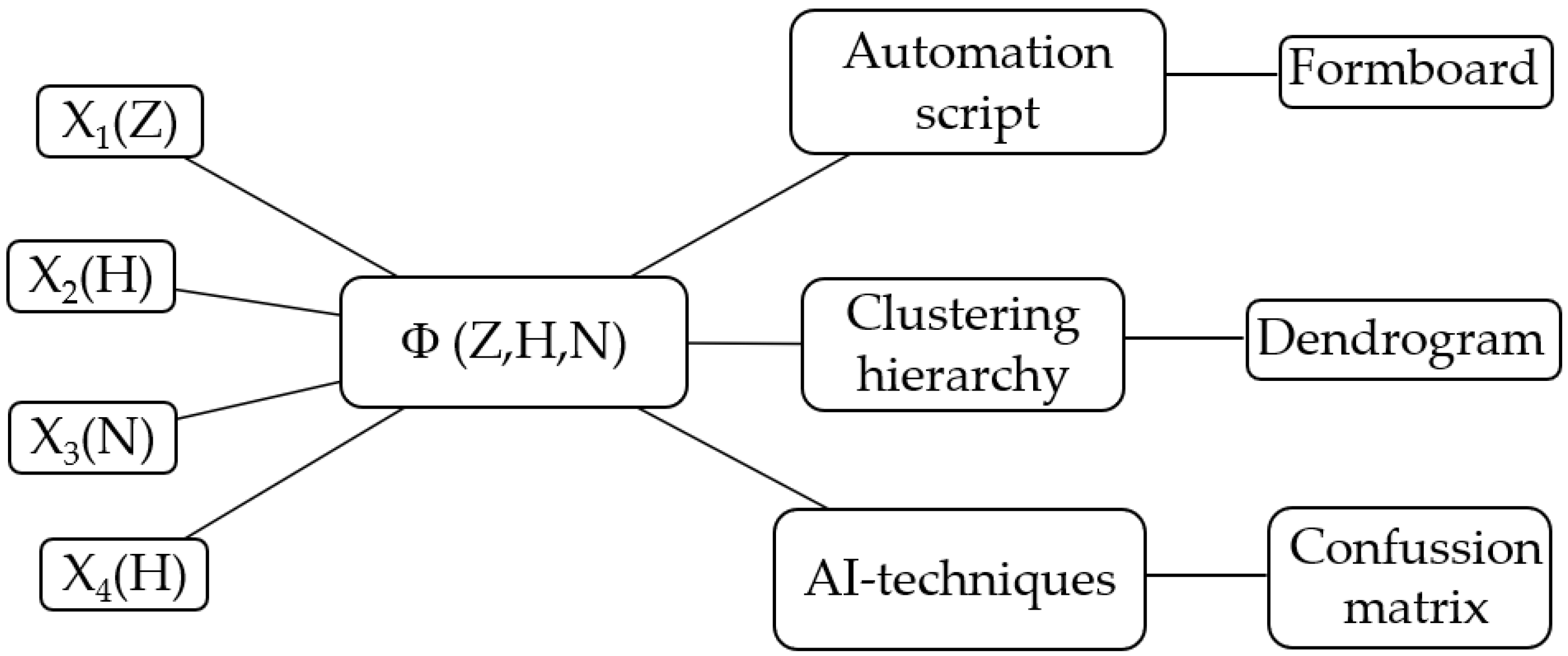
The risk matrix function, which represents a modern and effective approach to safety management, evaluates and prioritizes risks based on their likelihood and impact. The inputs/outputs of the AI model developed in this study are presented in Figure 1. The inputs to the system (${\mathrm{X}}_1,{\mathrm{X}}_2,{\mathrm{X}}_3,{\mathrm{X}}_4)$ are the factors related to the type of harness and the outputs include automation, predictions, and risk assessments to inform decision making in the engineering processes.

The dataset related to C295 aircraft consists of 157 electrical harnesses, which are obtained from the bill of material of each instance. It includes information about wiring length, number of electrical components, and electrical protection length. In total, in this study, the dataset includes 18,523 m of total wiring length, 21,200 electrical components, and 250 m of protective sheath length present in the 157 instances.

The functionality of the risk matrix provides features for identification of the risk in a more efficient manner. It is defined by categories such as low, medium, and high risk, which are established by assigning scores to each element of the dataset. Thus, data prioritization needs to be considered for immediate attention and mitigation. Overall, management of the risk provides information in real time in order to make the best decisions [31].

The new digital environment requires a holistic approach that integrates more automation and system interconnection. The latest implemented technology in industry 4.0 contains hi-tech strategies that enable sustainability by establishing connections between objects and interconnecting intelligent systems. The development of predictive innovative algorithms plays a key role in predicting error creation and achieving a better performance of the results [28]. Integrating AI methodologies into the manufacturing processes can enhance both efficiency and safety. The AI techniques used in this study include SVM, RF, LR, KNN, and XGBoost, which contribute to the analysis and results. SVM can be used for both data classification and regression. RF maintains accuracy from the average effect return of each individual tree. LR is used to estimate the probability of the binary outcomes. KNN presents high consistency in the results. XGBoost achieves high accuracy in predictions. Predictive algorithm functionalities, such as model evaluation, can be beneficial in assessing the performance of the model using appropriate metrics [32]. The appropriate selection of AI techniques to train the model and the continuous monitoring of the outcomes can be fundamental to make accurate predictions [33]. The predictive algorithm structure developed in this study is presented in Figure 1.

2.1. Automation Script

Complete automation is achieved by using a script that automates repetitive tasks necessary to turn the 3D harness model into a 2D manufacturing drawing. The developed automatic script includes the operations such as rotation of the electrical components and labeling of the electrical components. Other, more complicated operations such as rotation of the wiring, quick rolls, bends, and/or translation of the terminations are also automatically performed. This situation enables the automatic spreading of the 3D harness model into a 2D Formboard without errors [34].

Additionally, industrialization involves the creation of whole engineering documentation required for harness manufacturing. In traditional methods, this process is created from the perspective of the compliance with the requirements. In this new approach, a risk matrix function, which evaluates the likelihood of errors during the manufacturing process, is used. This assessment can be performed with five main dimensions: 3D model, the ‘Formboard’ (FB) defined as ${\mathrm{X}}_1$ representing the complexity of the 3D geometry, and ${\mathrm{X}}_2,{\mathrm{X}}_3,\mathrm{a}\mathrm{n}\mathrm{d} {\mathrm{X}}_4.$

Table 1. Criteria associated with each harness category associated with the risk matrix.

Description	Variables	Criteria	Cluster	Rule	Category
Formboard (FB)	${\mathrm{X}}_1$	Number of zones (Z)	Very large	Z > 100	5
			Large	60 < Z < 100	4
			Medium	20 < Z < 60	3
			Small	2 < Z < 20	2
			Very small	Z = 2	1
Technical Instructions (IT)	${\mathrm{X}}_2$	Number of wires (H)	Very large	H > 600	5
			Large	300 < H < 600	4
			Medium	100 < H < 300	3
			Small	10 < H < 100	2
			Very small	H < 10	1
Manufacturing Bill of Material (BOM) Electrical Test (ET)	${\mathrm{X}}_3$ ${\mathrm{X}}_4$	Number of components (N) Number of wires (H)
			Very large	N > 500	5
			Large	300 < N < 500	4
			Medium	100 < N < 300	3
			Small	20 < N < 100	2
			Very small	N < 20	1
			Very large	H > 600	5
			Large	300 < H < 600	4
			Medium	100 < H < 300	3
			Small	10 < H < 100	2
			Very small	H < 10	1

Table 1. Criteria associated with each harness category associated with the risk matrix.

Description	Variables	Criteria	Cluster	Rule	Category
Formboard (FB)	${\mathrm{X}}_1$	Number of zones (Z)	Very large	Z > 100	5
			Large	60 < Z < 100	4
			Medium	20 < Z < 60	3
			Small	2 < Z < 20	2
			Very small	Z = 2	1
Technical Instructions (IT)	${\mathrm{X}}_2$	Number of wires (H)	Very large	H > 600	5
			Large	300 < H < 600	4
			Medium	100 < H < 300	3
			Small	10 < H < 100	2
			Very small	H < 10	1
Manufacturing Bill of Material (BOM) Electrical Test (ET)	${\mathrm{X}}_3$ ${\mathrm{X}}_4$	Number of components (N) Number of wires (H)
			Very large	N > 500	5
			Large	300 < N < 500	4
			Medium	100 < N < 300	3
			Small	20 < N < 100	2
			Very small	N < 20	1
			Very large	H > 600	5
			Large	300 < H < 600	4
			Medium	100 < H < 300	3
			Small	10 < H < 100	2
			Very small	H < 10	1

2.2. Risk Matrix

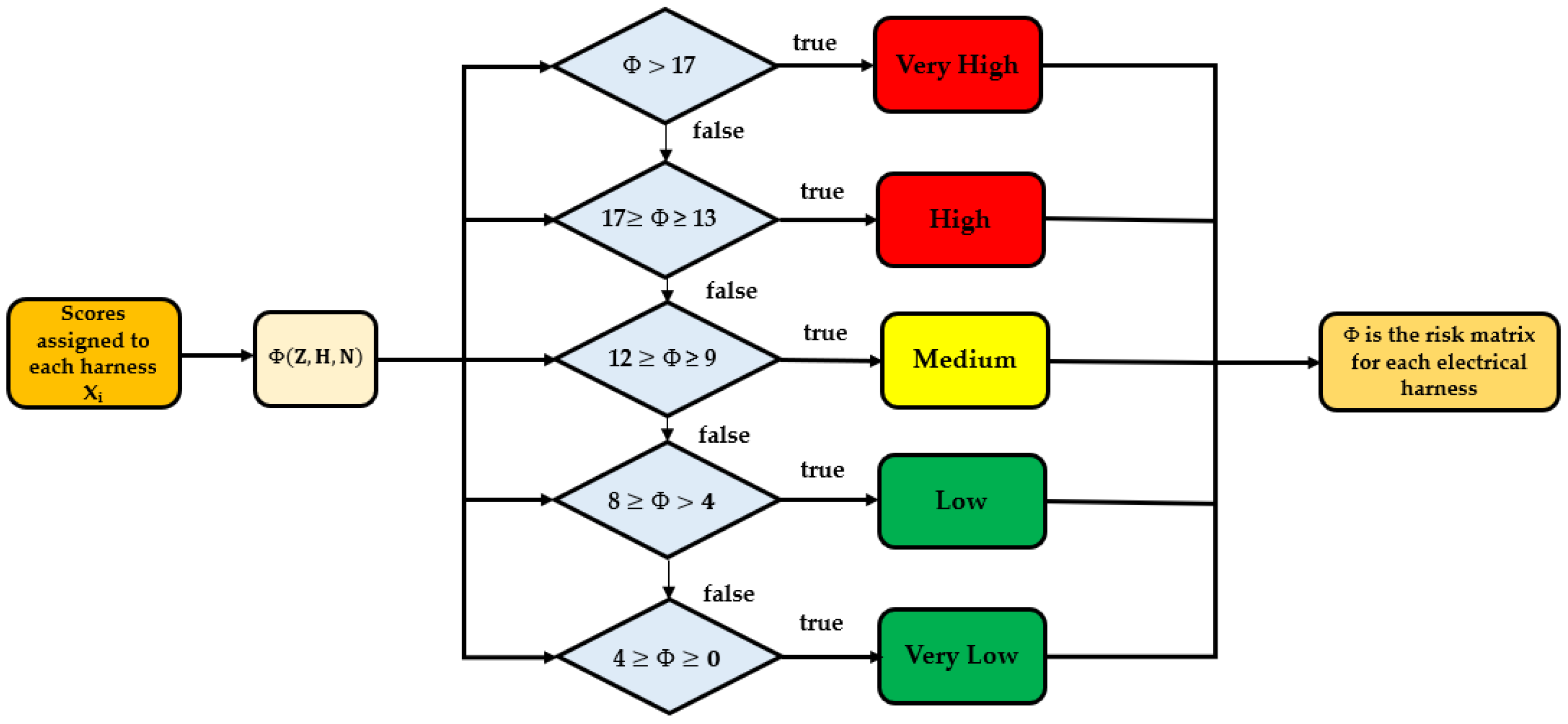
The complexity matrix for each of the harnesses was generated using input scores. The parameters which were used were determined by quantification of the number of zones (Z), number of wires (H), and number of electrical components (N) present in each harness dataset. The risk matrix function in an explicit form is represented in the following equation:

$$\mathrm{\Phi }\left(\mathrm{Z},\mathrm{H},\mathrm{N}\right)={\sum }_{\mathrm{i}=1}^4{\mathrm{X}}_{\mathrm{i}}={\mathrm{X}}_1\left(\mathrm{Z}\right)+{\mathrm{X}}_2\left(\mathrm{H}\right)+{\mathrm{X}}_3\left(\mathrm{N}\right){+\mathrm{X}}_4\left(\mathrm{H}\right)$$

(1)

The initiation of the kernel size, denoted as X_i, for the case study of the electrical harness in a military aircraft C295 follows the steps depicted in Figure 2. It shows the algorithm structure and highlights the different values of the risk matrix for each range associated with scores assigned to the dataset. A red color is assigned for a very high and high risk; yellow for a medium risk; and green for a low and very low risk of error creation.

The final score, as a sum of these values, determines the likelihood of error creation during the manufacturing engineering processes. Scores from 4 to 20 correspond from the simplest to the most complex geometry of the 3D electrical harness shown in

Table 2. Rule established to define risk matrix assessment in each harness.

Category	Rule	Risk Matrix
1	0 ≤ Φ ≤ 4	Very Low
2	4 < Φ ≤ 8	Low
3	9 ≤ Φ ≤ 12	Medium
4	13 ≤ Φ ≤ 17	High
5	Φ > 17	Very High

.

The risk matrix outcomes split the dataset into three main groups. The dataset is grouped into high, medium, and low risk of creating an error during the manufacturing process.

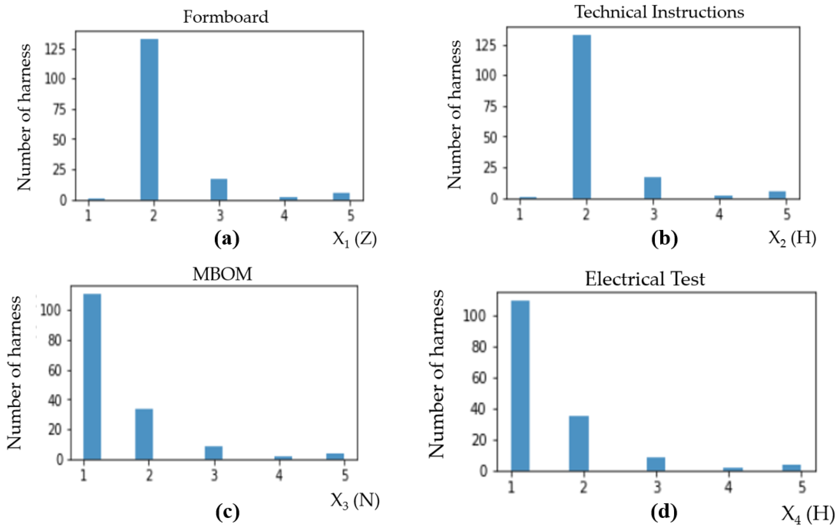
Histograms in Figure 3 show how the scores are assigned to the parameters ${\mathrm{X}}_1,{\mathrm{X}}_2,{\mathrm{X}}_3, \mathrm{a}\mathrm{n}\mathrm{d} {\mathrm{X}}_4$ in the case study of C295 military aircraft. From these histograms, only a very small percent of 3.8% of the dataset had scores of 4 and 5, which could potentially generate errors. The ability to focus attention on specific data or components rather than treating the entire system uniformly improves effectiveness in the processes. Clustering data will help to identify the features and similarities between them for failure anticipation. The clusters suggest that certain combinations of parameters can occur together, indicating relationships between these variables [35].

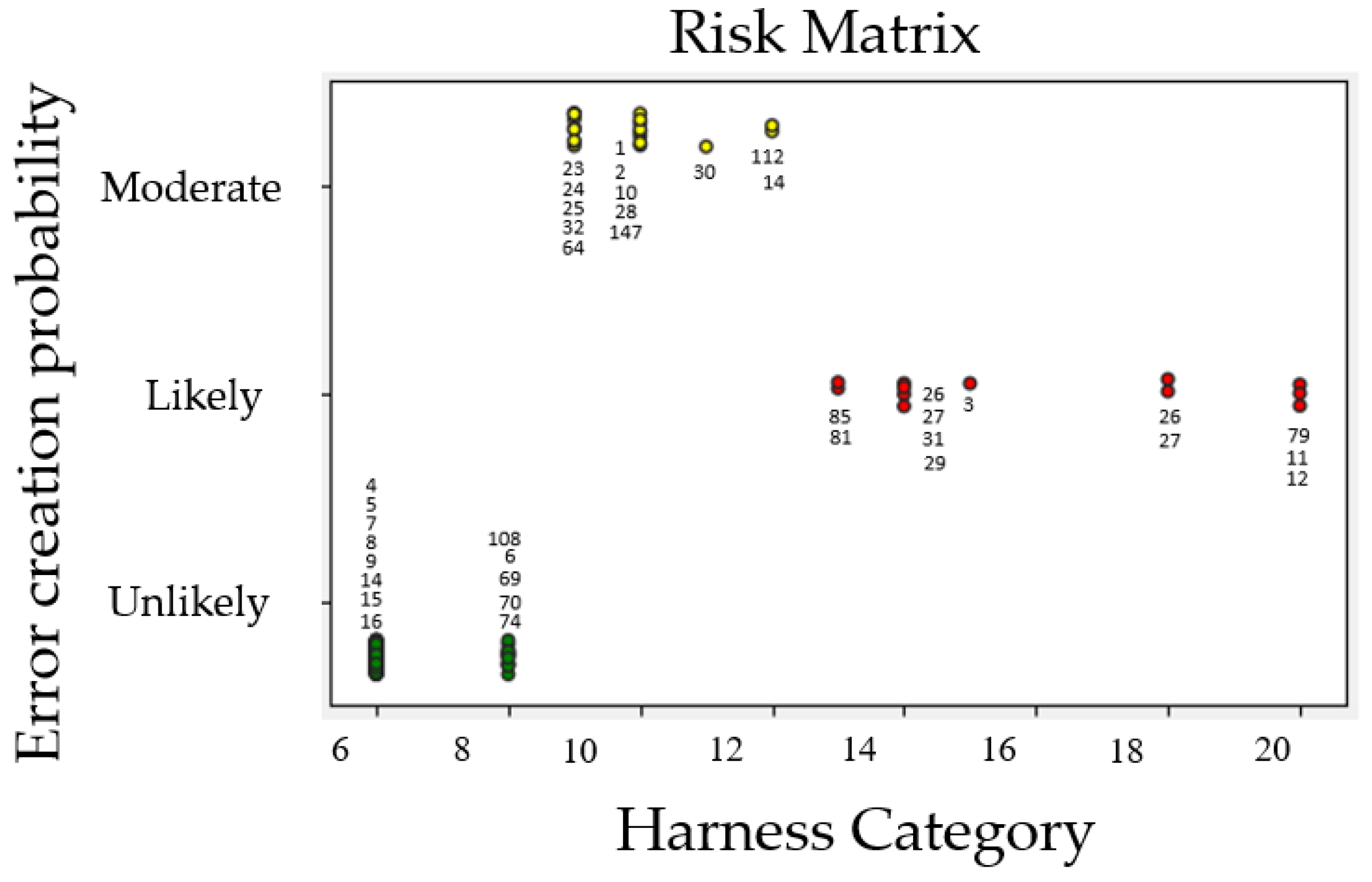
Figure 4 shows the risk matrix function evaluated for each harness within the dataset and the probability associated with the error creation during the manufacturing engineering processes in a color code.

2.3. Clustering Hierarchy

The main types of algorithms differ in the type of input/output data and scope of the problem that should be solved. Unsupervised algorithm techniques based on clustering are useful for application within the harness dataset. These techniques can be beneficial for identifying similarities and differences among harnesses, and therefore, for a more detailed analysis [27,35].

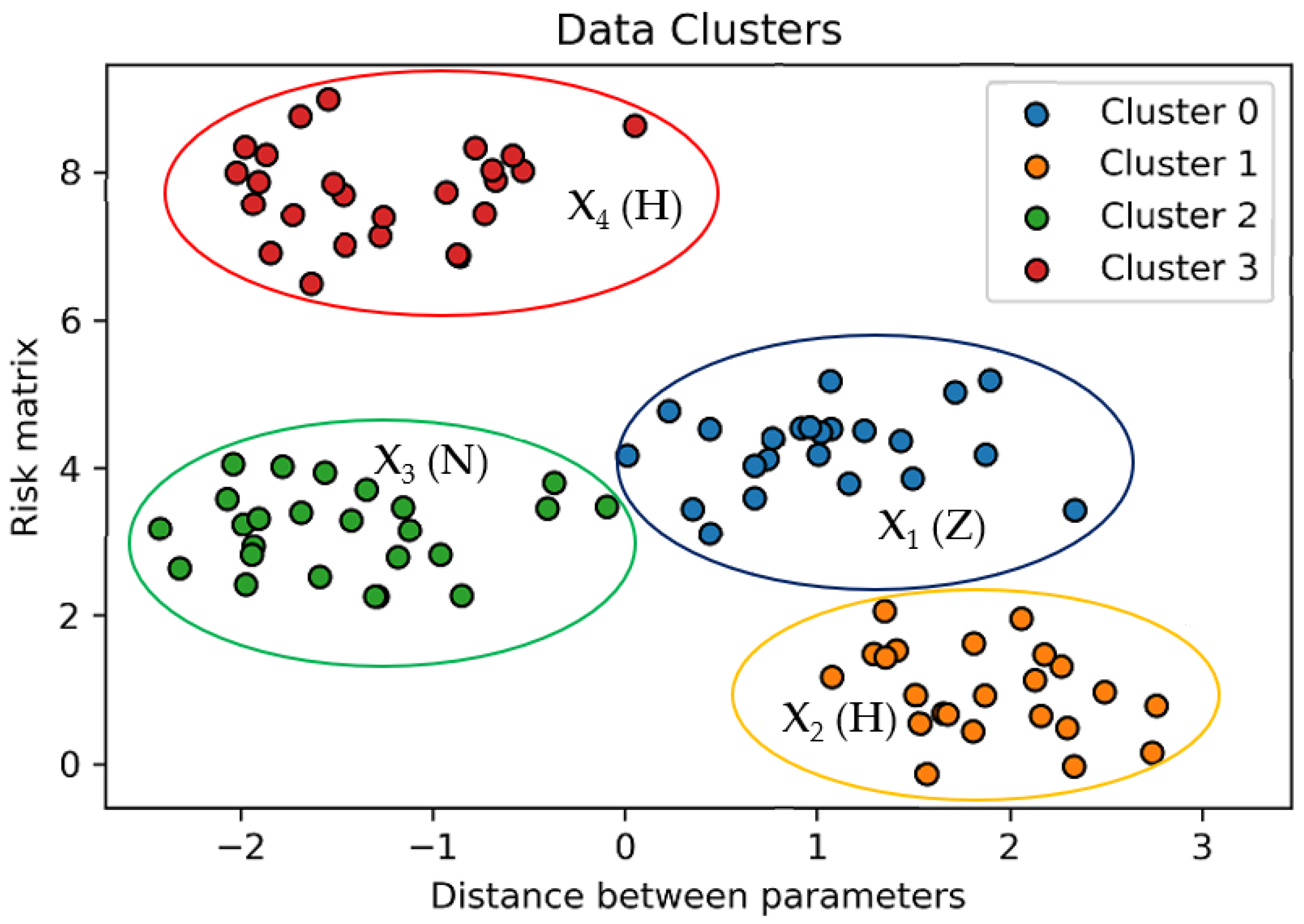
The algorithm used in this study applies clustering to analyze and to classify datasets. Figure 5 presents the clustering of data points defined by the risk matrix. Thus, ‘Formboard’ (FB) is represented by cluster 0 (in blue), ‘Technical Instructions’ (IT) by cluster 1 (in orange), ‘Manufacturing Bill of Material’ (MBOM) by cluster 2 (in green), and ‘Electrical Test’ (ET) by cluster 3 (in red).

The agglomerative clustering hierarchy uses input data defined as $A_1\cup \dots \cup A_j$ for the set for each observation in each cluster, with the following constraints:

$$\begin{gathered} A_1\cup \dots \cup A_j \mathrm{represents} \mathrm{the} \mathrm{number} \mathrm{of} \mathrm{clusters}. \\ {A}_j\cap { A}_{j’}=Ø \mathrm{no} \mathrm{overlapping} \mathrm{j} \ne \mathrm{j}’. \end{gathered}$$

The initialization of the clusters and merging process is as follows:

• Calculation of the proximity matrix, which represents the distances between each pair of data points based on the minimum distance: $\mathrm{d}\mathrm{m}\mathrm{i}\mathrm{n}=\sqrt{\sum _{\mathrm{i}=1}^{\mathrm{n}}{\left({\mathrm{q}}_{\mathrm{i}}-{\mathrm{p}}_{\mathrm{i}}\right)}^2}$, where p_i and q_i are coordinates of the data points.
• Identify two clusters with minimum distance.
• Merge the identified clusters into a new cluster combining the elements $A_1\cup \dots \cup A_j$.
• After merging two clusters, create a new cluster ($A_{new}$) represented as ${A_{new}=A}_1+A_j$, which contains elements of both clusters $A_1$ and $A_j$.
• Recalculate the distances between the new cluster and the remainder.
• Update the proximity matrix with the new distances.
• Continue this process iteratively.
• Repeat until the stop criterion is met with all elements merged in a cluster.

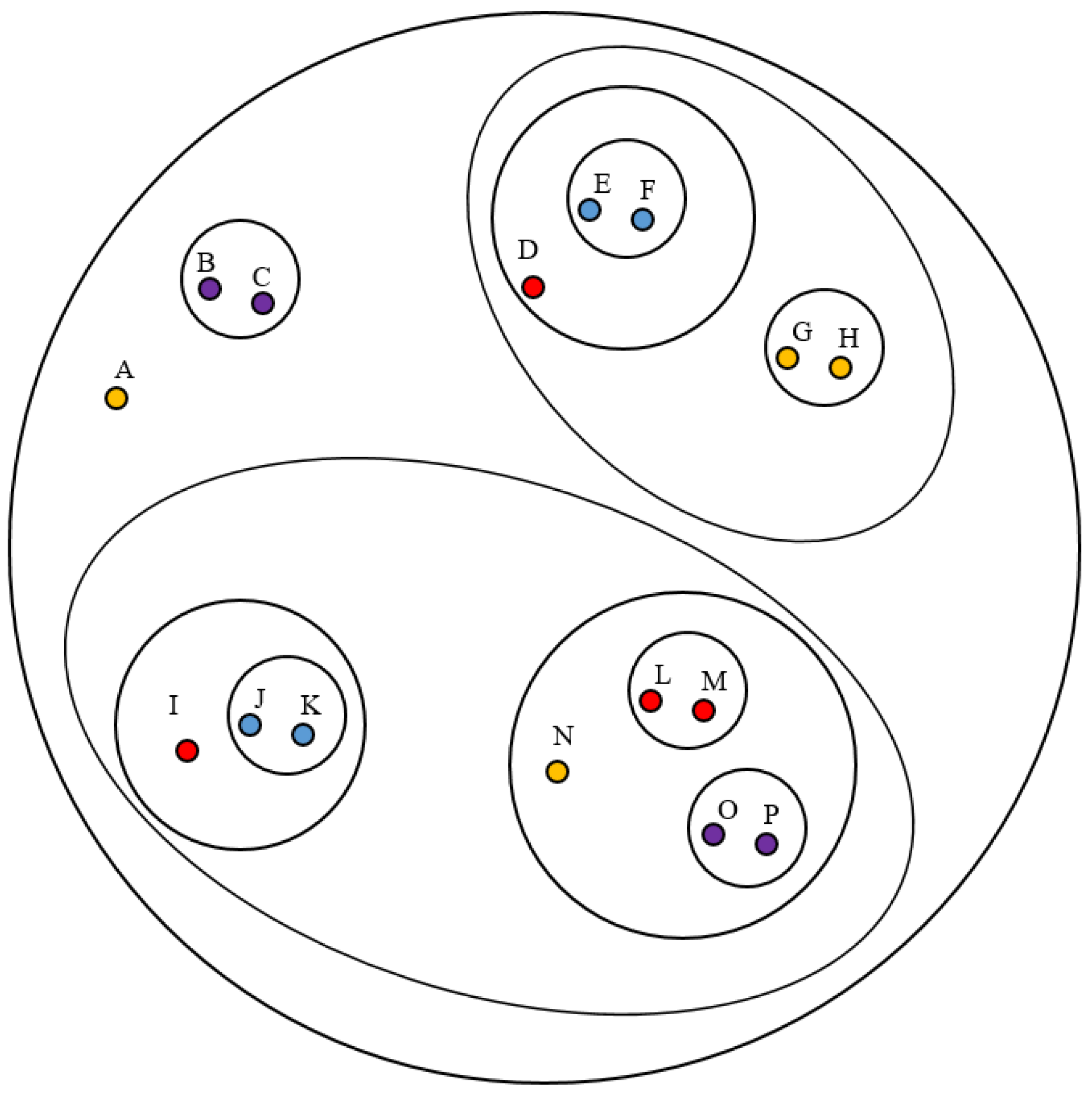
Figure 6 shows the merging process depicted as a dendrogram, which provides information about the critical clusters to be considered. Therefore, the dataset is grouped in families that give information about potential anomalies to be considered in order to anticipate error creation.

Hierarchical clustering establishes relationships between similar datasets grouped into clusters and labeled by letters from A to P.

2.4. Logistic Regression

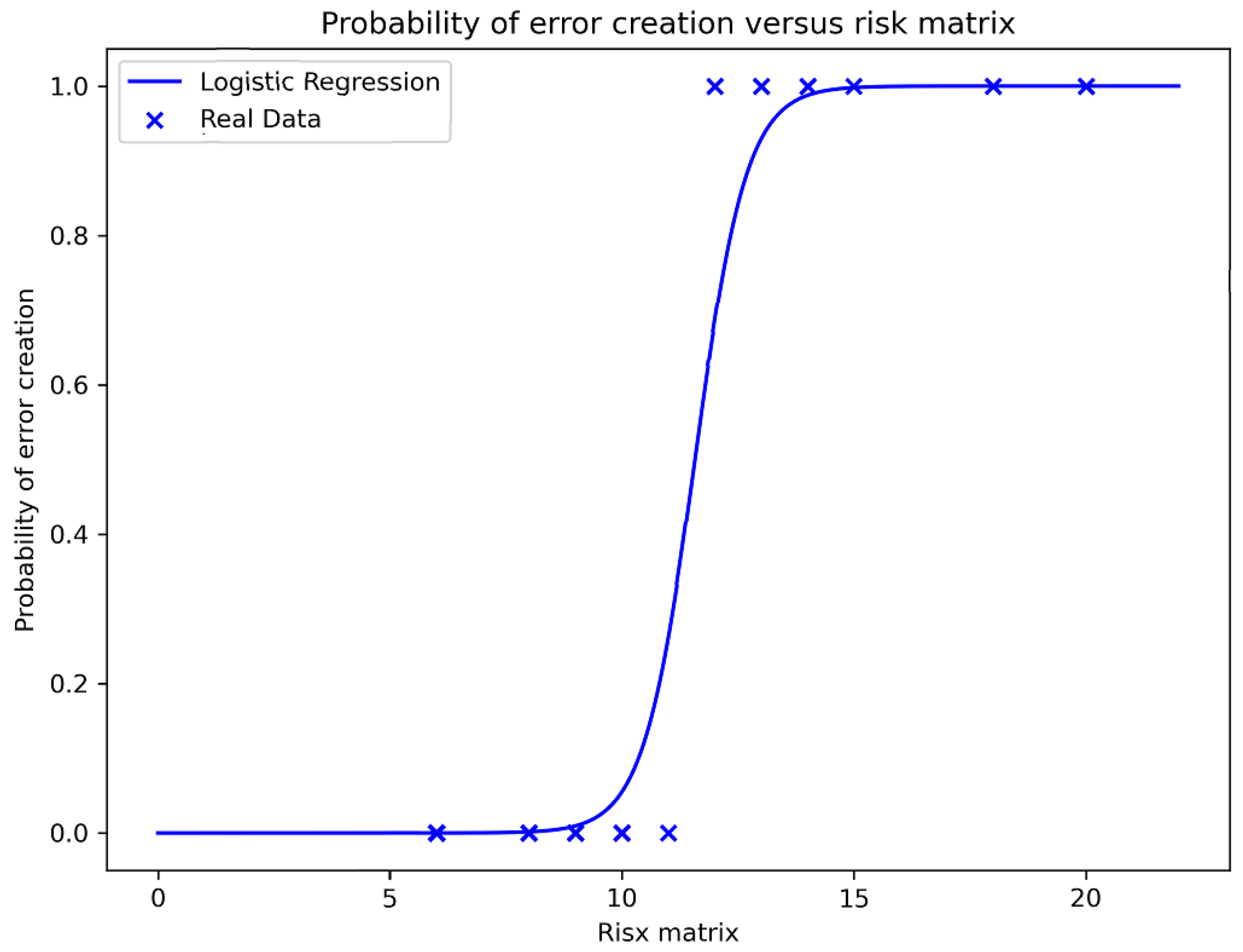
The best fit for the outcome categorical variable is defined by a logistic regression. Figure 7 represents the relationship between the probability of error creation and the risk matrix. The risk matrix function presents different values for each harness within the dataset. The probability function associated with the logistic regression is used for new data predictions. The logistic regression passes the input through the logistic/sigmoid function and then treats the outcome result as a probability [29].

2.5. Confusion Matrix

The confusion matrix considers the scores for each harness based on the number of zones (Z), number of wires (H), and number of components (N). The most important metrics in (2–5) are obtained from the confusion matrix as follows:

• Precision is defined as the ratio of correct positive predictions to the total number of positive predictions. This is the ratio between the real positive predictions and the total number of positives as the sum of true and false positives.
• The recall or sensitivity ratio is defined as the true positive prediction of the total number of positives. It is the ratio between real positives and real cases indicated as true positives or false negatives.
• Accuracy is defined as the ratio of the true prediction to the total value. It is the ratio of the total number of true positives and negatives in relation to the total number of real positives and real negatives within the dataset.
• The F₁ score is the harmonic mean of the precision and recall used to measure test accuracy. It varies from 1.0, showing perfect values of precision and recall, to 0, where either precision or recall is zero.

$$\mathrm{Precision}=\frac{\mathrm{TP}}{\mathrm{TP}+\mathrm{FP}}$$

(2)

$$\mathrm{Recall} \mathrm{or} \mathrm{sensitivity}=\frac{\mathrm{TP}}{\mathrm{P}}=\frac{\mathrm{TP}}{\mathrm{TP}+\mathrm{FN}}$$

(3)

$$\mathrm{Accuracy}=\frac{\mathrm{TP}+\mathrm{TN}}{\mathrm{P}+\mathrm{N}}=\frac{\mathrm{TP}+\mathrm{TN}}{\mathrm{TP}+\mathrm{TN}+\mathrm{FP}+\mathrm{FN}}$$

(4)

$${\mathrm{F}}_1=\frac{2}{\frac{1}{\mathrm{Precision}}+\frac{1}{\mathrm{Recall}}}=\frac{2 \mathrm{TP}}{2 \mathrm{TP}+\mathrm{FP}+\mathrm{FN}}$$

(5)

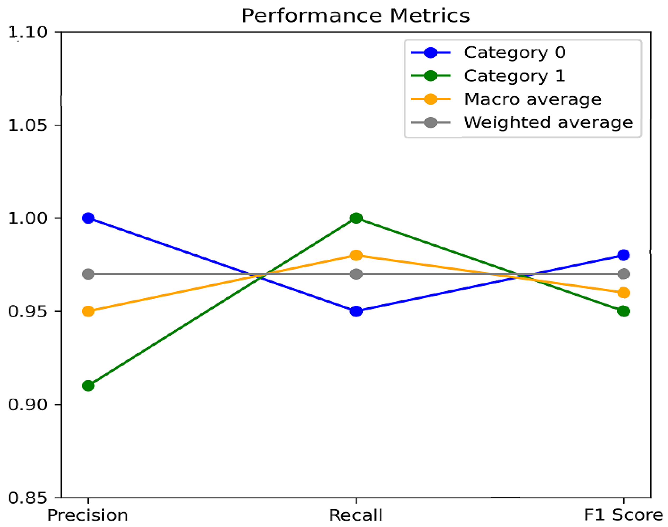
In addition, the machine learning classification report provides some additional values as outcomes. Category 0 represents the negative class that means ‘no error creation’, and category 1 represents the positive class, meaning ‘error creation’. The macro-average is the average of the precision, recall, and F₁-score. The weighted average is the weighted average of the precision, recall, and F₁ scores, as shown in

Table 3. Classification reports of machine learning metrics such as precision, recall, and F₁-score, with macro- and weighted average.

Category	Precision	Recall	F1-Score
0	1.00	0.95	0.98
1	0.91	1.00	0.95
Accuracy	-	-	0.97
Macro-average	0.95	0.98	0.96
Weighted average	0.97	0.97	0.97

. The performance metrics are depicted in Figure 8.

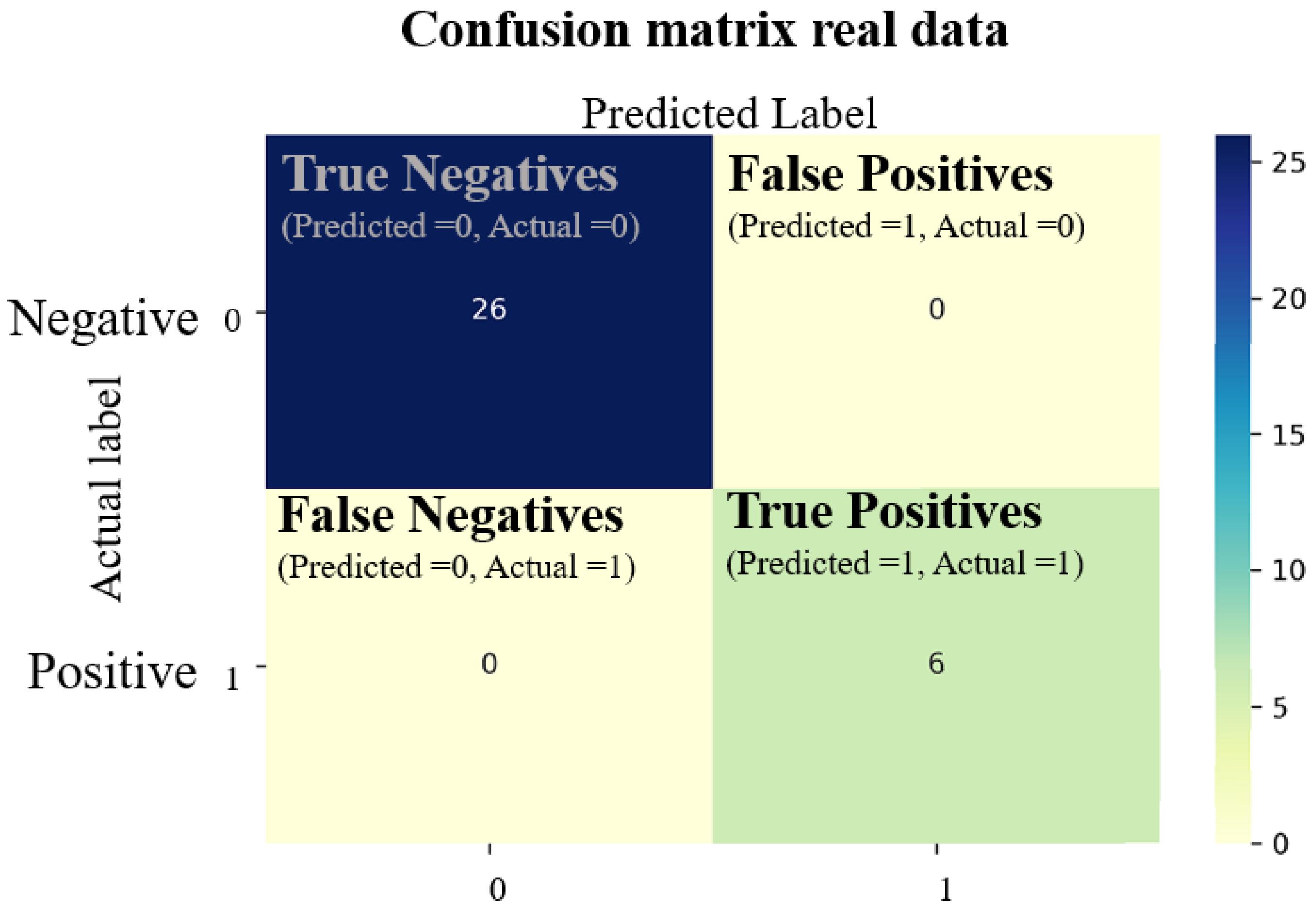
The algorithm splits the dataset into two subsets: training set and test set. The training set was used to fit the model, and the test set was used to evaluate the performance of the model through the confusion matrix as shown in Figure 9.

From the confusion matrix, the predictions show the good performance of the algorithm. True positives (TP): Prediction is a value that matches reality. The element at (1,1) represents the six data samples as true positives classified as ‘error creation’. True negatives (TN): The prediction value also matches reality. The element at (0,0) represents the 26 data samples as true negatives classified as ‘no error creation’. The diagonal elements represent the instances that are correctly classified. False positives (FP) and false negatives (FN) are off-diagonal elements representing the number of instances incorrectly classified.

3. Results and Discussion

3.1. Statistical Analysis

3.1.1. Time Savings

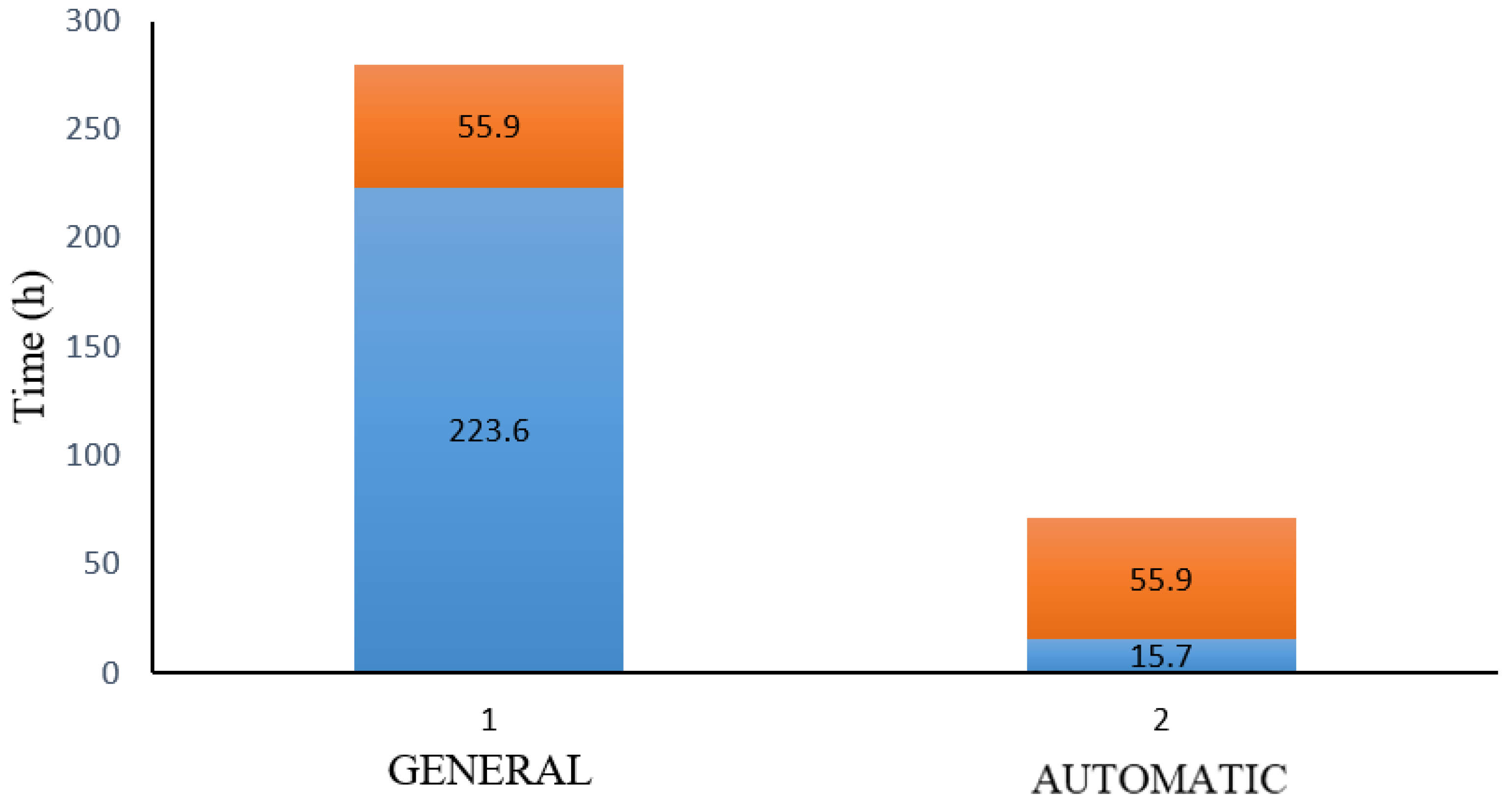
The time savings are achieved through the automation of electrical harness operations, such as rotations, rolls, and straightens, and by the assistance provided during drawing creation, such as label designation, symbols, and manufacturing annotations. The operational time allocated for data preparation is a constant defined as ε in (6). It is calculated for the entire dataset in this study as 55.7 h for both general and automatic procedures. However, the operational time σ(t), used during documentation creation, is defined as a function that depends on time. In the general procedure, the necessary time to perform these operations is 223.6 h versus the 15.7 h established in the automatic procedure. Thus, a reduction of 93% in time was estimated. The time calculation values for both procedures are outlined in

Table 4. Time calculation comparison between general procedure and automatic script.

$\mathsf{\tau }\left(\mathbf{t}\right)$
Activity	$\mathsf{\epsilon }$				$\mathsf{\sigma }\left(\mathbf{t}\right)$
	Flattening Model	Flattening Parameters	Data Extraction	Harness Flattening	EHF Operations	Drawing 2D
					Branches Arrangement	Designations Labels
					Branches Rotation	2D Annotations
					Roll	Symbols
					Straighten	Other
General Procedure	13.9	13.8	14.3	13.9	223.6
Automatic Script	13.9	13.8	14.3	13.9	15.7

.

$$\mathrm{T}\left(\mathrm{t}\right)=\mathsf{\epsilon }+\mathsf{\sigma }\left(\mathrm{t}\right)$$

(6)

The graph depicted in Figure 10 shows a comparison between the operational time in the general procedure and the automatic procedure using a bar representation to visualize the time savings achieved by the automation process. The time drops from 223.6 h to 15.7 h, shown as a blue bar in Figure 10, which generates a reduction of 93% in the time for the entire electrical dataset in this military aircraft. $\mathsf{\epsilon }$ = 55.9 h shown as an orange bar in Figure 10 is the sum of all the constant operational times necessary to be performed using both procedures for the entire dataset.

3.1.2. Sensitivity Analysis

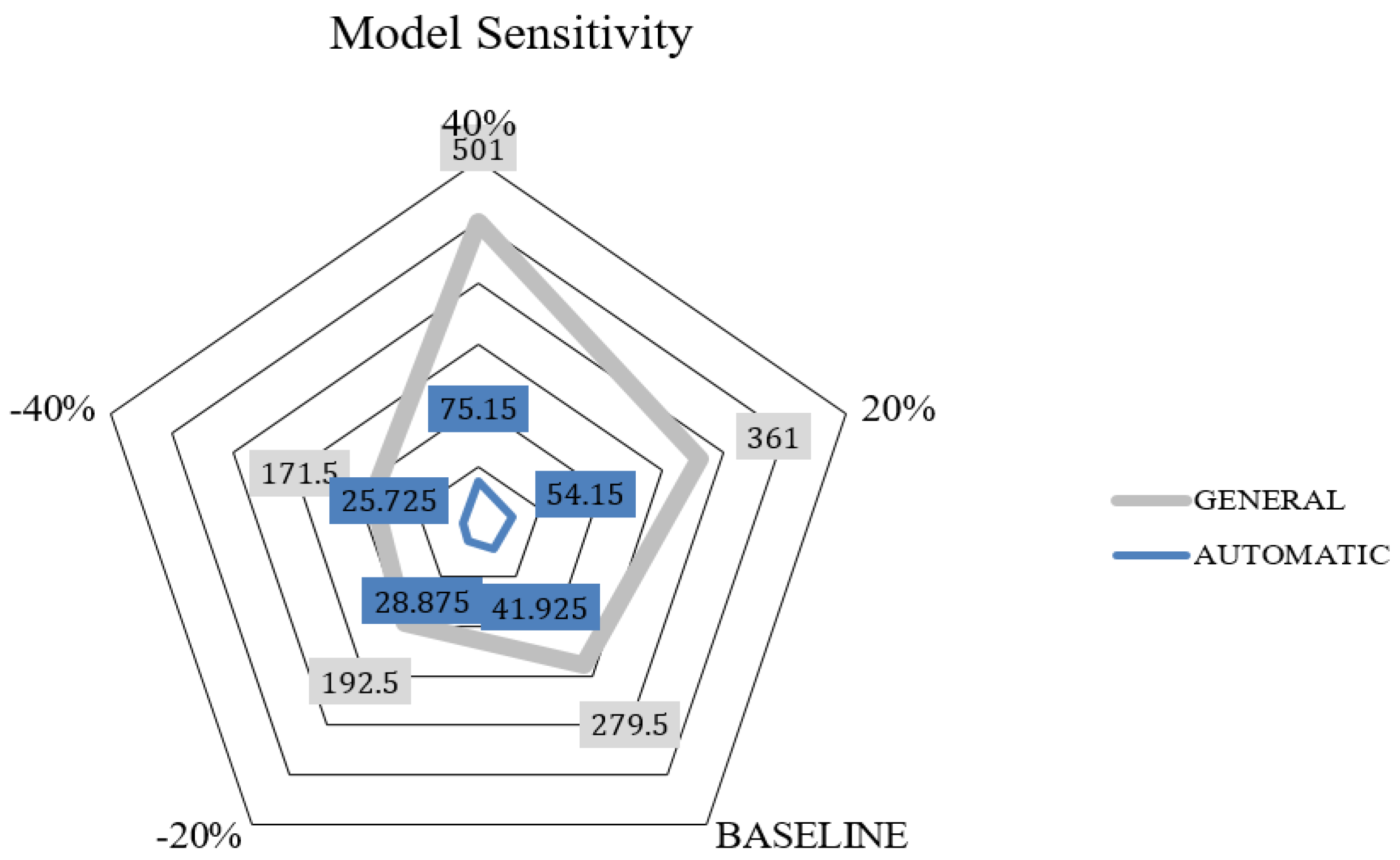
Sensitivity analysis is performed to analyze the influence of variations in the input parameters on the time prediction of the AI model developed in this study. This approach is used to evaluate the robustness and reliability of the model [22]. The evaluation is based on the variation in input parameters across two different scenarios, and the impact generated on the model outputs. The key parameters identified that are used as inputs are the number of wires (H), terminations (Z), and electrical components (N). The variation is established systematically over a range of values in each of the electrical harness datasets varying from ±20% to ±40%. After assessing parameter variation, the next step is to analyze how the changes affect the outputs. Figure 11 depicts the savings in time achieved on a general and automatic procedure from baseline to a range of input parameter variations of +20%, +40%, −20%, and −40%. The assessment of the output changes, with regard to the baseline of the total time of 279 h defined in the creation of the manufacturing documentation, establishes a variation from the maximum value of 501 h at a +40% level of sensitivity to the minimum of 171.5 h at −40% in a general procedure. The automation procedure shows a baseline of 41.92 h and a variation from 75.15 h at a 40% level of sensitivity to 25.72 h at −40%. The parameter values either increased or decreased after the sensitivity test was performed, showing consistency in the output changes. This situation provides a good estimation of the likelihood of the parameter predictions, since an increment in the percentage of the values means a greater number of wires, more components, more harness complexity, and therefore a higher risk matrix and higher probability of error creation. Consequently, the time estimation for both procedures increased following an escalation in the input parameters. Likewise, the situation presents the opposite effect whether or not the values of the parameters decrease. The consistent behavior produces reliable results and gives evidence of the robustness of the model. Therefore, sensitivity analysis enhances confidence in the predictions of the model. The quantitative measures show consistency in model behavior and are evidence to validate model reliability and robustness.

3.1.3. Correlation Parameters

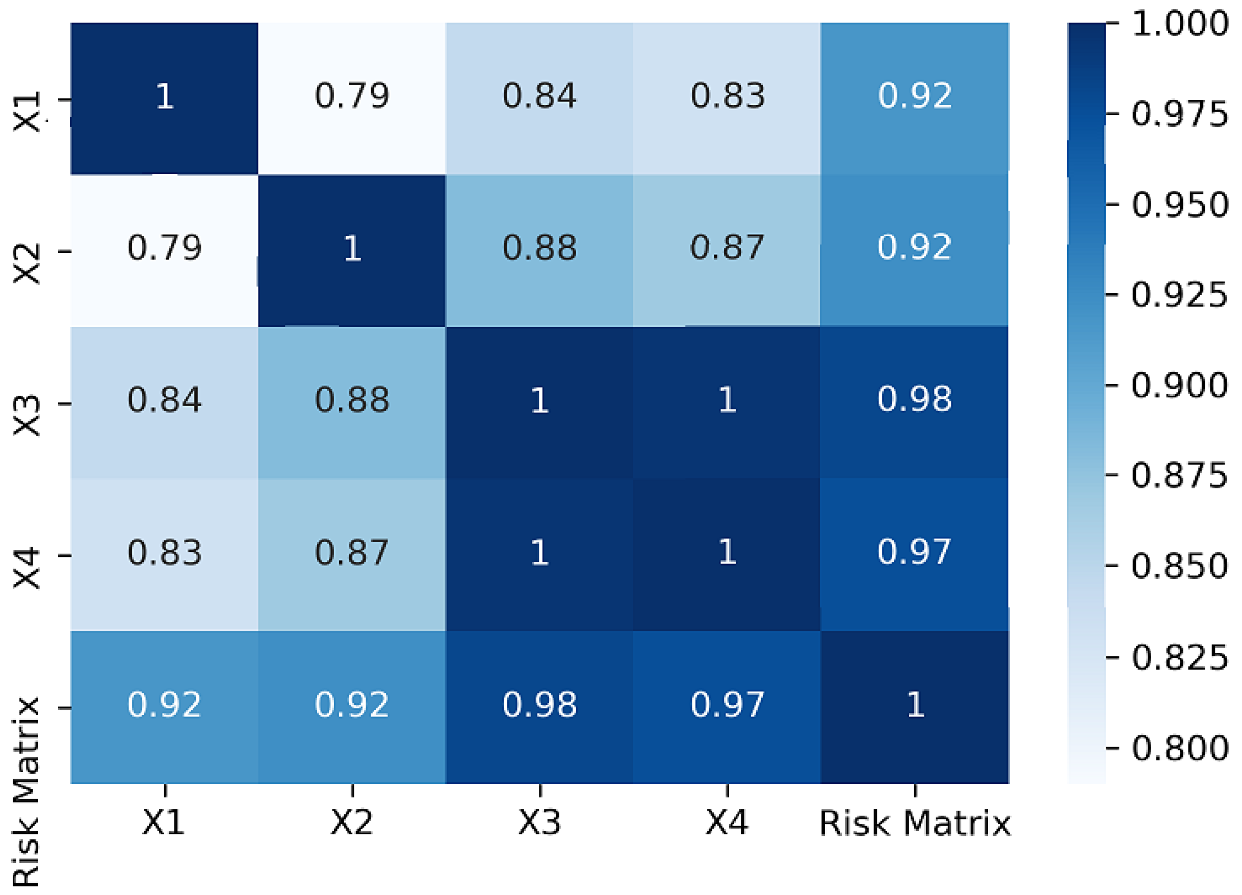
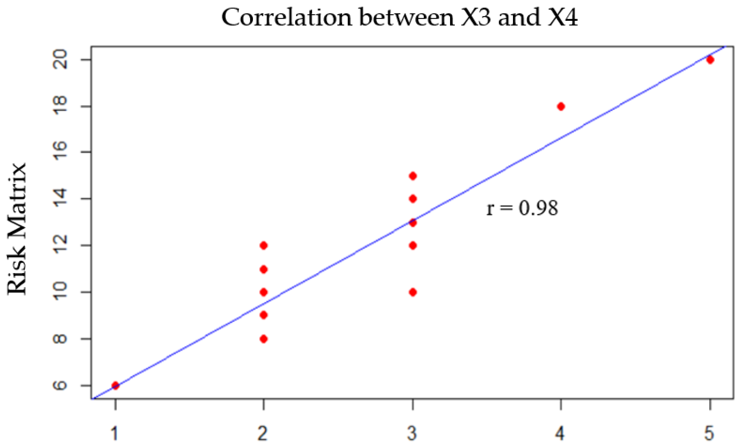
The correlation parameter analysis is performed to measure the strength and direction of the relation between each parameter and the risk matrix. The coefficients indicate that the closer to one the absolute values of the coefficients are, the stronger the correlation is. Consequently, an increase in a parameter can lead to an increase in the risk matrix. Figure 12 quantifies the relationship between input parameters showing that the variables are highly positively correlated. The correlation of the variables was quantified by calculating the Spearman correlation coefficient, which evaluates the relationship between the input parameters of the dataset. The parameters that present the highest influence on the risk matrix are ${\mathrm{X}}_3$ and ${\mathrm{X}}_4$ at 0.98 and 0.97, respectively. The higher the correlation presented within the parameters is, the greater the likelihood of error creation during the manufacturing processes is. Thus, variations in these parameters directly affect the outcomes of the predictive model. The Spearman coefficient provides valuable insights and can inform about the decision-making process which is related to error prediction. The existing correlation between parameters ${\mathrm{X}}_3$ and ${\mathrm{X}}_4$ demonstrates the impact on the risk matrix function, which is fundamental to analyzing the probability of error creation and defining strategies for risk mitigation. The calculation of each coefficient parameter ‘r’ in Equation (10) is represented in the correlation matrix, whose values are calculated using Equations (7)–(9) for each pair of variables.

$$\mathrm{C}\mathrm{o}\mathrm{v}(\mathrm{x},\mathrm{y})=\sum \left[\left({\mathrm{X}}_{\mathrm{i}}-{\mathsf{\mu }}_{\mathrm{x}}\right)\left({\mathrm{Y}}_{\mathrm{i}}-{\mathsf{\mu }}_{\mathrm{y}}\right)\right]/\mathrm{n}-1$$

(7)

$${\mathsf{\sigma }}_{\mathrm{x}}=\sqrt{\left[\sum {\left({\mathrm{X}}_{\mathrm{i}}-{\mathsf{\mu }}_{\mathrm{x}}\right)}^2\right]}/\mathrm{n}-1$$

(8)

$${\mathsf{\sigma }}_{\mathrm{y}}=\sqrt{\left[\sum {\left({\mathrm{Y}}_{\mathrm{i}}-{\mathsf{\mu }}_{\mathrm{y}}\right)}^2\right]}/\mathrm{n}-1$$

(9)

$$\mathrm{r}=\frac{\mathrm{c}\mathrm{o}\mathrm{v}\left(\mathrm{x},\mathrm{y}\right)}{{\mathsf{\sigma }}_{\mathrm{x}}{\mathsf{\sigma }}_{\mathrm{y}}}$$

(10)

Figure 13 represents the highest positive correlation between ${\mathrm{X}}_3$ and ${\mathrm{X}}_4$ and the risk matrix. It is observed that low scores assigned to these parameters generate a moderate risk matrix with scores between 8 and 14, which is mostly the situation expected in the dataset present for this light and medium aircraft. There are only a few scores that strongly impact the risk matrix, pointing at 18 and 20. It also shows a positive linear tendency between both parameters and the risk matrix. In summary, ${\mathrm{X}}_3$ and ${\mathrm{X}}_4$ are the parameters that most affect the outcomes of the model. Therefore, these parameters must be treated as critical parameters. The interpretation of the correlation parameter impacts the effectiveness of risk management strategies. Correlation results are valuable in explaining the influence of the parameters on error prediction and risk mitigation. Understanding the relationships between variables can influence the decision-making process. Identifying variables, which are significant, can provide effective risk mitigation strategies. Analyzing potential risks or vulnerabilities from certain variables can help in taking preventive measures and avoiding errors.

3.1.4. Error Prediction

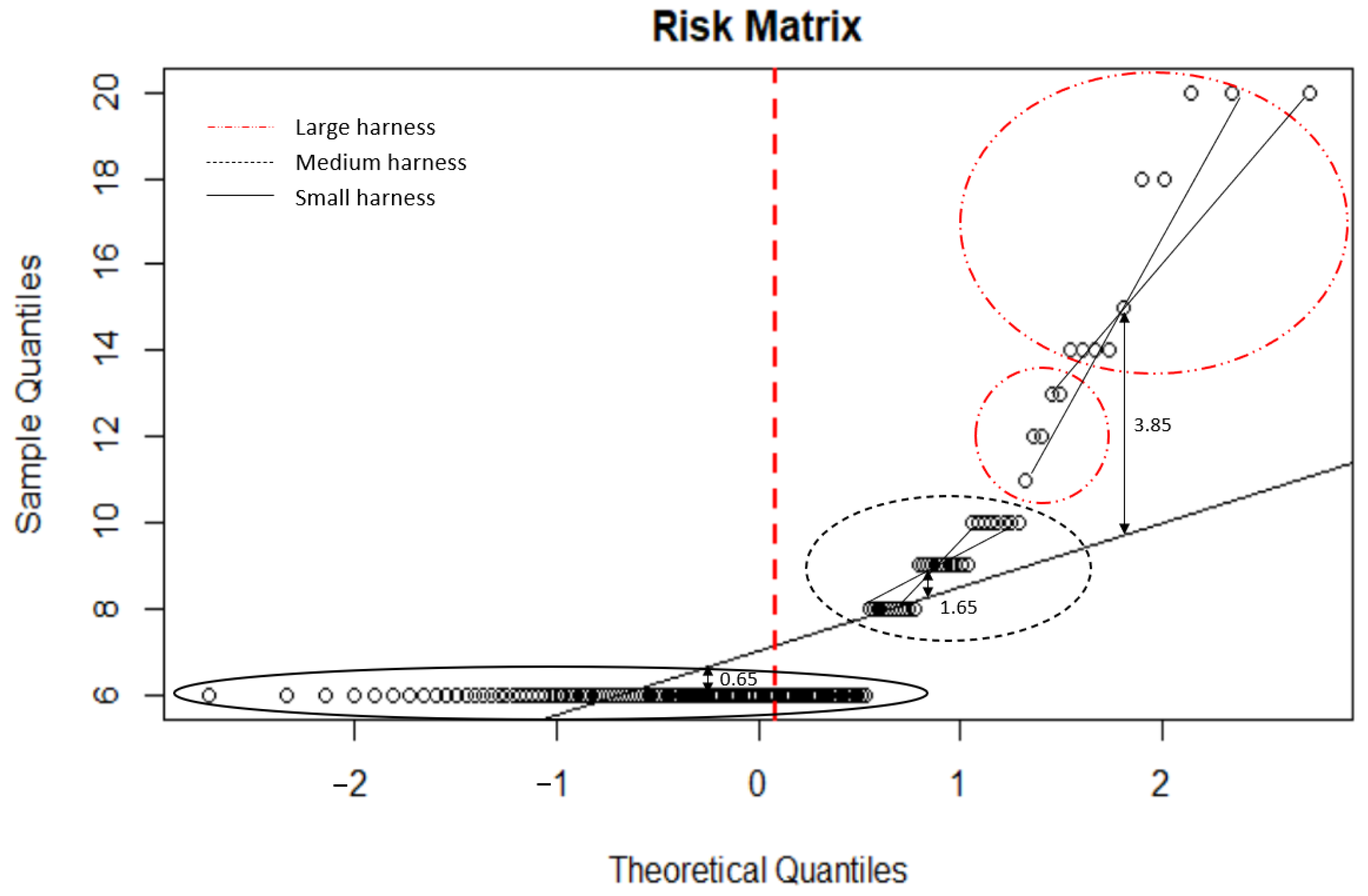
Error prediction analysis is performed to understand factors that can contribute to error creation. Figure 14 compares the distribution of the dataset to a theoretical distribution, such as a normal distribution. The theoretical quantile is compared against the sample quantiles to assess whether the data closely follow a normal distribution. The normal distribution dataset is represented by the tendency line. The greater the fit to the points through this line, the closer the fit is to a normal distribution. The dataset was divided into three groups: small, medium, and large harnesses. The first cluster shows a low impact in the risk matrix, and the dataset points present a risk matrix below 6, in the case of small harnesses. The second cluster shows a medium impact on the risk matrix between 8 and 10, for medium harnesses. The third cluster shows a high impact in the risk matrix between 11 and 20, for large harnesses.

The comparison of the dataset with a normal distribution is used to make decisions about the process. After data representation, the distribution of the dataset in clusters, and the fitting to the theoretical standard normal distribution, the maximum deviation occurs at cluster 3 with 3.85 units from the center of the data distribution above the tendency line, as shown in Figure 14. The vertical red line evaluates how the dataset deviates from the expected theoretical behavior represented by the tendency line.

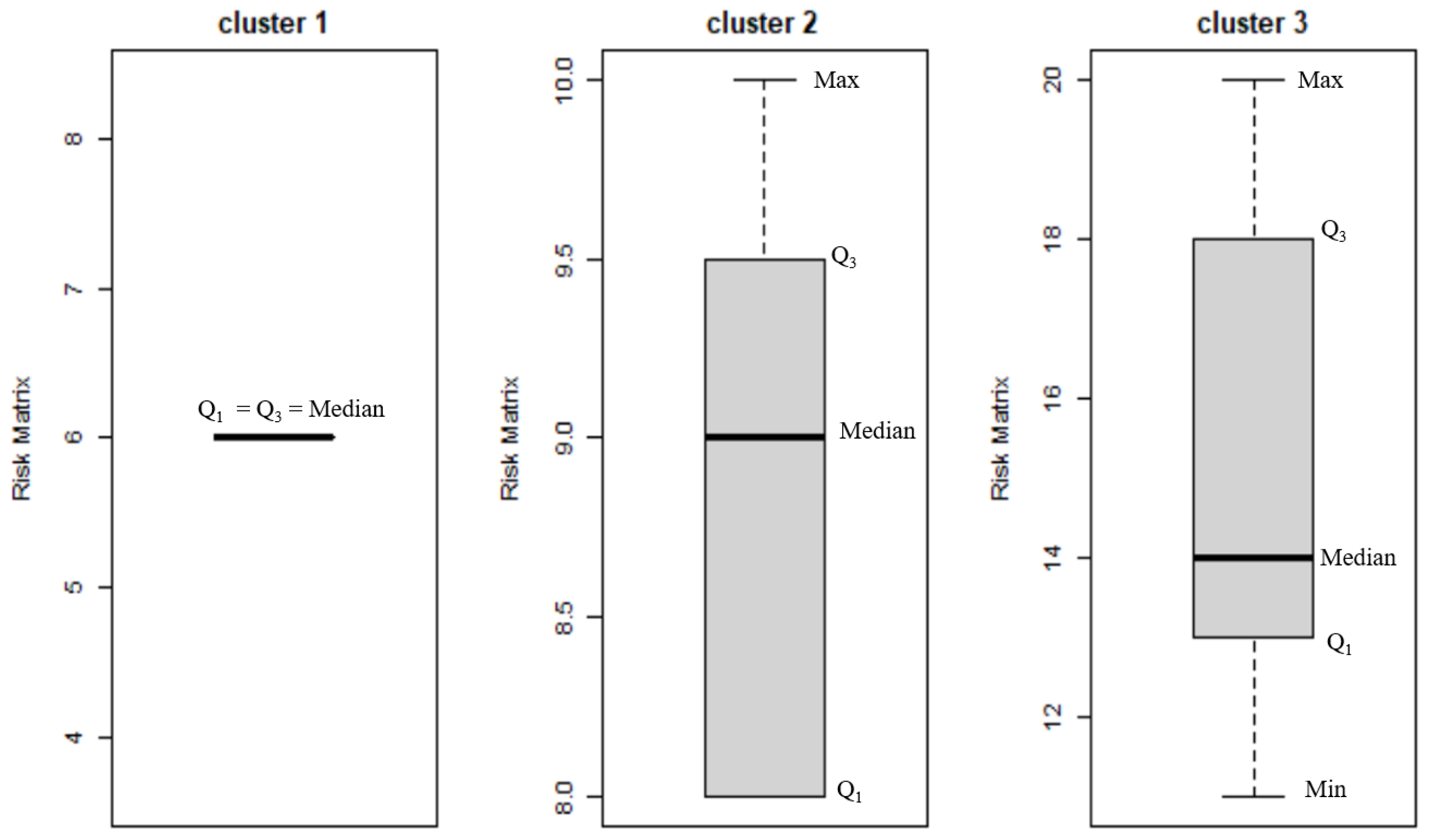
Figure 15 represented by the box-plots show how close the distribution of a dataset is to an ideal distribution using quartiles.

In the first cluster, the first quartile Q₁ and third quartile Q₃ match together, showing the same risk matrix outcome from the data points within this group. In the second cluster, the median is represented at a risk matrix value of 9.0, showing a positive skew slightly deviated from the normal distribution. The median of the second cluster is 0.25 above the median of the ideal normal standard distribution. In the third cluster, the median is represented at a risk matrix value of 14, which shows a negative skew. The median of the third cluster is 1.5 below the median of the ideal normal standard distribution.

Box-plot results show the data distribution which is crucial for predicting error creation and establishing risk mitigation strategies. Skewed data distributions may require special attention to ensure robust modeling and data prediction. Cluster 3 presents more skew data than cluster 2. The accuracy of the statistical analysis and predictions can be affected depending on the skewness due to loss of symmetry of the data distribution. The highest deviation occurs in cluster 3, generating the highest impact in the risk matrix and therefore in the evaluation of error creation with 3.85 units above the tendency line of a normal distribution. Additionally, for reliability purposes, the proposed methodology developed in this study was validated using a Monte Carlo simulation as an effective approach to assess the reliability of the model [36].

3.2. Proposal Method Comparison with AI Existing Techniques

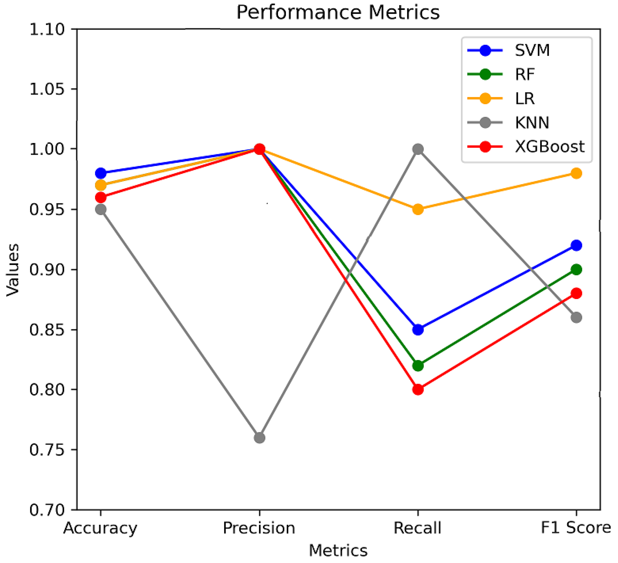
This study used the logistic regression (LR) for predictions since it indicates good performance between precision and recall, as shown in

Table 5. Performance metrics comparison between proposed LR and other AI methods.

Model	Accuracy	Precision	Recall	F1-Score
SVM	0.98	1.00	0.85	0.92
RF	0.97	1.00	0.82	0.90
LR	0.97	1.00	0.95	0.98
KNN	0.95	0.76	1.00	0.86
XGBoost	0.96	1.00	0.80	0.88

. The efficiency of this method is proved by comparison with the existing techniques such as SVM, RF, KNN, and XGBoost.

Figure 16 represents the performance metrics such as accuracy, precision, recall, and F₁-score obtained using different techniques. The highest accuracy is obtained using SVM. The highest precision is achieved using SVM, RF, LR, and XGBoost. The highest recall is obtained using KNN and the highest F₁-score is obtained using LR.

The LR has shown very good performance in comparison to other proposed, existing techniques in terms of F₁-score. It may not have the highest accuracy but its overall performance suggests that it can be the best choice. SVM may be a good choice since it has achieved the highest accuracy and precision; however, the recall is lower than LR.

3.3. Experimental Verification

In order to verify the accuracy of the proposed methodology, we have compared the performance of AI methods using model data of this study and experimental data presented by ElDali and Kumar 2021 [37]. The experimental datasets used the Commercial Modular Aero-Propulsion System Simulation (C-MAPSS) and Prognostics and Health Monitoring (PHM08) generated by NASA Ames Research Center (Mountain View, CA, USA). The datasets contain features related to a total of 435 aircraft engines from sensor measurements. The sensor values were selected according to the metrics presenting the highest suitability to define failure patterns. The measurements were used for predictions of the remaining useful lifetime of the aircraft engines and their fault estimation. To verify the performance of our model, we have applied AI methods including SVM, RF, LR, KNN, and XGBoost to the measurement datasets of the sensors. Each AI algorithm is used to determine its effectiveness using technical data (TD) from input parameters of this study and measured data from the sensors (SM). The performance metrics are represented in

Table 6. Performance metrics comparison obtained using different AI methods between technical dataset (TD) and sensor measurement (SM).

Metrics AI Methods	Accuracy		Precision		Recall		F1-Score
	TD	SM	TD	SM	TD	SM	TD	SM
SVM	0.98	0.95	1.00	1.00	0.85	0.88	0.92	0.94
RF	0.97	1.00	1.00	1.00	0.82	1.00	0.90	1.00
LR	0.97	1.00	1.00	1.00	0.95	1.00	0.98	1.00
KNN	0.95	0.95	0.76	1.00	1.00	0.88	0.86	0.94
XGBoost	0.96	1.00	1.00	1.00	0.80	1.00	0.88	1.00

.

The difference between SM and TD in accuracy is up to 4% for SVM, RF, LR, and XGBoost. The accuracy obtained using KNN is the same on the measured and model values. The measured and modeled precision is the same for all the methods, except for KNN, which shows a difference of 24%. The recall shows a difference up to 18% between SM and TD. The F₁-score presents a difference up to 12%. The analysis reveals that SVM and LR have consistently performed, showing the smallest deviation between measured and model values for all metrics. Overall, the experimental values are aligned with the modeled ones, which proves the good performance of the developed model in this study.

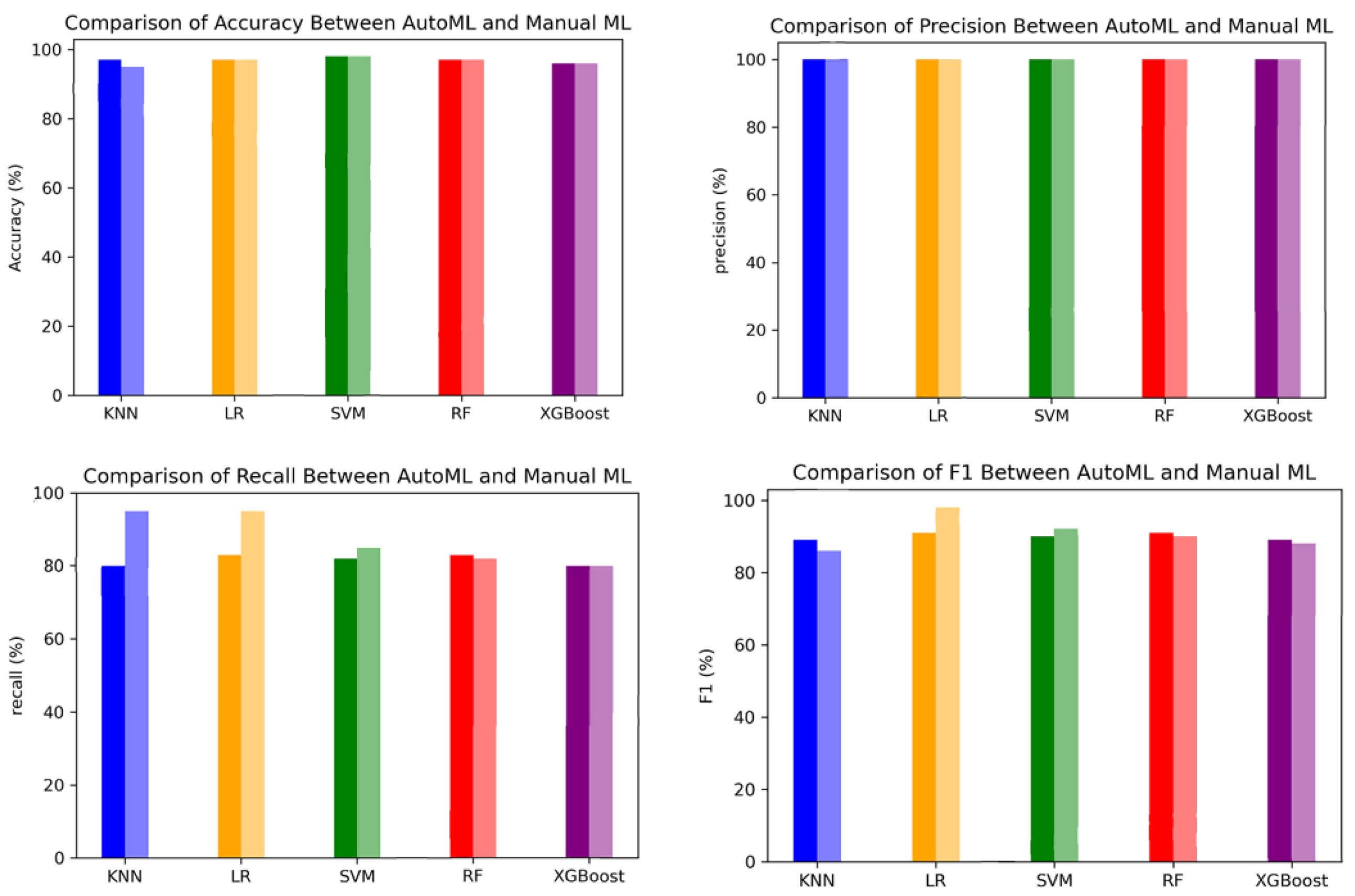
3.4. Advancements in Machine Learning

The process involved in the simulation of the AI algorithms includes the necessary steps to ensure optimal model performance and accurate predictions. Data preprocessing is necessary to ensure that the input data are appropriate for model training. Additionally, the most suitable AI techniques need to be selected, which depend on the characteristics of the dataset. Also, it is crucial to optimize selected hyperparameters in order to establish an appropriate set up for the AI model proposed. Moreover, visualizations of the model performance metrics are necessary to assess the model accuracy and effectiveness. Thus, Automated Machine Learning (AutoML) can be a valuable tool to perform the entire process automatically. To assess the effectiveness and suitability of the selected AI methods, we have compared the traditional machine learning approach with AutoML. We have used the same input data for both traditional and AutoML models. The AutoML frameworks include tools such as H₂O-AutoML, DataRobot, Cloud AutoML, the Tree-based Pipeline Optimization Tool (TPOT), Auto-Keras, Auto-Weka, ML BOX, AutoSklearn, and Auto-Pytorch [38,39,40,41]. In this study, we have used the TPOT, which uses a Genetic Algorithm (GA) to automatically find which AI methods present the best performance for the dataset [42]. We have compared performance metrics of the AI methods including SVM, RF, LR, KNN, and XGBoost for both AutoML and traditional approaches. The results are presented in Figure 17.

Figure 17 shows the performance metrics obtained using AutoML and traditional ML for each of the AI methods proposed. In each graph, the darker-colored bars represent the metrics obtained using AutoML and the lighter-colored bars represent the metrics using manual ML. The highest deviation appears in recall in KNN, showing a difference of 15% between AutoML and the manual approach. LR presents the highest difference of 12% in recall. The methods SVM, RF, and XGBoost show a difference up to 3% in recall and F₁. The results show that leveraging AutoML can find the best classifier while reducing the time invested in manual ML.

We use the k-fold cross technique to validate the performance of the AI methods proposed. Such a technique splits the dataset into k-folds. The TPOT evaluates the model on each fold in order to estimate the performance more accurately. The TPOT also uses the value of k = 5, splitting the dataset into five equal parts. Each fold is used as a validation set while the remaining four are used for training. It evaluates the model five times in order to assess the performance of the different AI methods. This value balances the performance accuracy and the computational effort.

Table 7. Performance metrics of the best pipelines using k-fold cross-validation.

K-Folds	Accuracy	Precision	Recall	F1-Score
1st-fold	97	97	97	97
2nd-fold	96	96	96	95
3rd-fold	96	96	96	95
4th-fold	95	95	95	94
5th-fold	96	97	97	97
6th-fold	96	96	96	96
7th-fold	95	96	95	95
8th-fold	95	96	95	95
9th-fold	94	95	94	94
10th-fold	93	94	93	93
Average	95	96	95	95

presents the metrics of the best pipelines using a 10-fold cross-validation. These metrics indicate that the best pipelines proposed by the TPOT provide an average accuracy, recall, and F₁-score of 95%, while the average for precision is 96%.

3.5. Discussion

Logistic regression is used for classification of the dataset and the evaluation of model performance by a confusion matrix. The logistic regression can evaluate the significance of the input parameters and the potential impact in the output model. Thus, a powerful predictive algorithm can forecast error creation in order to avoid errors. Simultaneously, errors in engineering documentation are mitigated. Therefore, validation of the results can provide evidence to enhance process efficiency and reliability at electrical manufacturing in aerospace and overall safety in aviation.

The dataset from the statistical analysis shows a Spearman coefficient of 0.98, which demonstrates that the variables are highly positive correlated. The box-plot representation shows that the dataset outcomes present a deviation above the tendency line compared to an ideal normal distribution of 3.85 in a large harness cluster, 1.65 in a medium one, and 0.65 in a small one. AI results based on failure anticipation methods show that the highest probability within the dataset to create errors in engineering processes are presented by the high-risk matrix. A 90% reduction in error creation has been achieved by the AI model developed in this study. The highest correlation is presented between ${\mathrm{X}}_3$ and ${\mathrm{X}}_4$ parameters with the ‘risk matrix’ at values of 0.98 and 0.97, respectively. Additionally, a sensitivity analysis shows good prediction results, proving the robustness and reliability of the model. The parameter variation shows consistency in the model outputs and are proved to validate model reliability and robustness of the model.

Furthermore, the flexibility presented by the risk matrix can accommodate other types of risk. The proposed approach can be generalized to other disciplines such as healthcare, energy, and automotives. Healthcare can gain the benefit of using the risk matrix, which offers real-time information to the surgeons about the level of risk they will face during the surgical procedure. This approach can provide the detection and prevention of failures. Additionally, it can also provide prioritization on which patient to act on in terms of mortality, in order to save their lives. In the energy sector, the risk matrix can be used to analyze the hazards associated with equipment failures to enhance safety strategies or mitigate losses by implementing more efficient processes. Furthermore, the risk matrix can play a key role in product safety in the automotive industry. The assessment of the risks can be useful in reducing the accident rate and decreasing production time. With the increasing digitalization of automotives, the risk matrix can also be useful in assessing cybersecurity threats.

The use of AutoML can play a key role in automatically finding an appropriate model which provides reliable forecasts for data prediction. The accuracy and effectiveness of the predictive models used can be improved without the need of extensive human intervention. For future directions, in spacecraft systems, considering existing constraints related to limited data availability, uncertainty in values, and the need for real-time decisions can be very beneficial to use. However, continuous research and innovation will be necessary to apply AutoML to aerospace applications and reach the highest accuracy.

4. Conclusions

In this study, AI techniques are applied to design predictive algorithms capable of predicting and mitigating potential failures in the aerospace manufacturing processes. The decision-making aspect implies the assessment of the risk of error creation by a risk matrix function. This approach has the potential to enhance efficiency, reduce errors, and contribute to overall improvements in the aerospace manufacturing domain.

The integration of AI techniques into the manufacturing design process for electrical harnesses enhances systems reliability, improves the performance of electrical systems, and improves error mitigation, making it well suited for aerospace. The AI results can be used to identify nonlinear data behavior and complex patterns within the dataset, enhancing confidence in the models’ outputs. After comparing different AI techniques, such as SVM, RF, LR, KNN, and XGBoost, the best performance is obtained from logistic regression (LR). Therefore, LR is used for output predictions. Integrating AI techniques, logistic regression provides a rigorous analysis of the model behavior and enhances the reliability of the proposed approach.

The experimental verification analysis demonstrated that LR, RF, and XGBoost show high performance. These AI methods are feasible for predicting errors and mitigating risks of aerospace systems. The experimental values are aligned with the modeled ones, which provides evidence of the good performance of the model approach in this study. This analysis indicates that SVM and LR have shown the smallest deviation up to 5% between measured and model values for all metrics.

The use of AutoML has also provided evidence to obtain the best metrics of the selected AI methods. The results have shown that the performance metrics obtained using AutoML and traditional ML are comparable. However, leveraging AutoML can enhance the choice of the best classifier, while reducing the time used in manual ML.