Abstract
Aggressive flight has become increasingly important for expanding the applications of quadrotors. The typical characteristic of large and rapid changes in commands poses stringent demands on the maneuverability of quadrotors. Ensuring flight stability alone is not enough; dynamic responses must also be selectively constrained, presenting quadcopter flight control with daunting challenges. The prescribed performance control (PPC) method is seen as having the potential to solve this problem by allowing for the constrained control of specified performance, leading to extensive research. However, its practical application still faces challenges, such as the system divergence caused by errors exceeding boundaries due to sudden command mutations. This paper presents a robust dynamic event-triggered PPC (DETPPC) method for an aggressive quadrotor flight. By assessing the direction and proximity of tracking errors approaching constraint boundaries, a dynamic event-triggered compensation mechanism for performance function boundaries is established to mitigate the divergence caused by error surpassing and to preserve preset control over the targeted metrics. Controllers were designed for both the translational and rotational subsystems of the quadrotor, and stability analysis was conducted based on Lyapunov functions. Simulation tests on agile trajectory tracking and abrupt attitude control were carried out, demonstrating the effectiveness of the proposed method.
1. Introduction
In recent years, the application scenarios of quadrotors have expanded into military reconnaissance, strike missions, and commercial aerial performances [1,2,3]. Unlike traditional low-speed or hovering flights, in such applications, commands can change on a large scale, rapidly, or even abruptly [4]. For instance, in military reconnaissance, the tracked target may suddenly evade, necessitating rapid changes in speed and direction by the quadrotor to maintain tracking. These are all typical characteristics of an aggressive flight, imposing stringent demands on the maneuverability of quadrotors and posing challenges to flight control.
During an aggressive flight, quadrotors experience high speeds, rapid attitude changes, and noticeable aerodynamic disturbances, leading to pronounced model nonlinearity and uncertainty [5]. This poses a formidable challenge for the design of quadrotor flight controllers, primarily due to the difficulty of balancing maneuverability and robustness. Existing flight control methods and research, such as backstepping-based control [6], sliding-mode-based control [7], adaptive-based control [8], and neural-network-based control [9], primarily focus on enhancing quadrotors’ robustness against model errors and external disturbances for stable flight [10]. However, they lack attention to and constraints on quadrotors’ transient performance. Combining adaptive nonlinear control with disturbance observers, some studies have been able to achieve finite-time error convergence and ultimately maintain uniformly bounded tracking. However, their convergence speed heavily relies on the initial error. Especially when the initial error is substantial, the convergence time is inevitably longer [11].
To achieve a better transient response aligned with specified constraints, prescribed performance control (PPC) has gradually emerged in quadrotor flight control [12]. It utilizes a prescribed performance function to guide tracking errors to converge in a predetermined residual region within defined constraints, such as maximum overshoot, convergence time, and allowable tracking deviation. Therefore, the design of the specified performance function is crucial, representing a focal point in recent research on PPC. Jia [13] and Veiginis [14] refined the basic performance constraint function based on initial error, allowing for adjustable constraint levels. However, their practicality is limited by the understanding of the initial system states. Such methods are not applicable when the initial error is unknown or the actual situation deviates from the preset initial conditions, such as sudden disturbances or different task instructions. Overly conservative designs can result in slow responses. Bu [15] and Xiao [16] improved control efficiency for nonlinear systems by introducing hyperbolic tangent and exponential functions, creating a performance constraint independent of initial tracking errors. However, the independence from initial conditions may lead to excessive system overshooting in cases of loose initial conditions. In quadrotor applications, Xu et al. [17] integrated PPC with adaptive dynamic programming, enabling finite-time attitude constraint control under external disturbances. Shao et al. [11] established a threshold-triggered expanded state observer based on PPC, enabling adjustments of quadrotor attitude under specific overshoot conditions. Wang et al. [18] integrated PPC with backstepping, accounting for coupling between translational and rotational subsystems, enabling precise position tracking of quadcopter quadrotors with minimal overshoot. However, while the above-mentioned studies quantitatively constrain the targeted indicators, singular problems arise when errors exceed the performance envelope. Therefore, Wang [19] and Hu [20] addressed the issue by introducing terms related to the derivative of the command in the prescribed performance function, allowing constraints to adapt based on changes in task states. However, it is usually difficult to obtain the command form expressed in time. Particularly for abrupt commands like step signals or error steps induced by sudden disturbances, the method becomes inapplicable. But, these situations are extremely common, even typical, in quadrotor aggressive flights. Therefore, to leverage the advantage of PPC in constraining specific performance and improve the control effect of a quadrotor aggressive flight, it is necessary to endow its performance function with the ability to adapt to the out-of-bounds caused by sudden errors.
Drawing inspiration from the above, in this paper, we propose a dynamic event-triggered prescribed performance control (DETPPC) method and design controllers for the translational and rotational subsystem of the quadrotor. Subsequently, the boundedness and stability of the controller based on Lyapunov functions were proved. Moreover, attitude control and aggressive trajectory tracking simulations were conducted under command mutations and external disturbances to demonstrate the effectiveness of the proposed method. The main contributions of this paper are summarized as follows.
- A dynamic event-triggered performance function boundary adaptive adjustment mechanism is proposed. By assessing the error variation direction and its distance from the performance function boundary, a dynamic compensation factor related to input commands and current errors is established for the performance function, preventing the system divergence caused by errors exceeding the performance function.
- A robust control framework based on DETPPC is established. Based on this, we designed the controller for the quadrotor translational and rotational subsystems by separately constructing unconstrained error dynamics and performance functions incorporating a dynamic event-triggered compensation factor. Furthermore, stability analysis was conducted based on Lyapunov functions.
- Attitude control and aggressive trajectory tracking simulations were conducted under command mutations. The results demonstrate that, compared to traditional PPC and cascade PID methods, the proposed DETPPC controller avoids the system divergence caused by errors exceeding the performance function and achieves a faster response and convergence, as well as reduced oscillations.
Based on the above, our method not only preserves the preset constraints on the quadrotor transient performance but also innovatively enhances flight robustness and algorithm practicality by addressing the divergence caused by errors exceeding the performance function during command changes. The following is the content arrangement of this paper. Section 2 gives the problem formulation and preliminaries, including the quadrotor model and the control objective. The design of the dynamic event-triggered prescribed performance function is presented in Section 3. Section 4 and Section 5 construct controllers and stability analysis, respectively. Section 6 presents the simulation and discussion, while the conclusion is given in Section 7.
2. Problem Formulation and Preliminaries
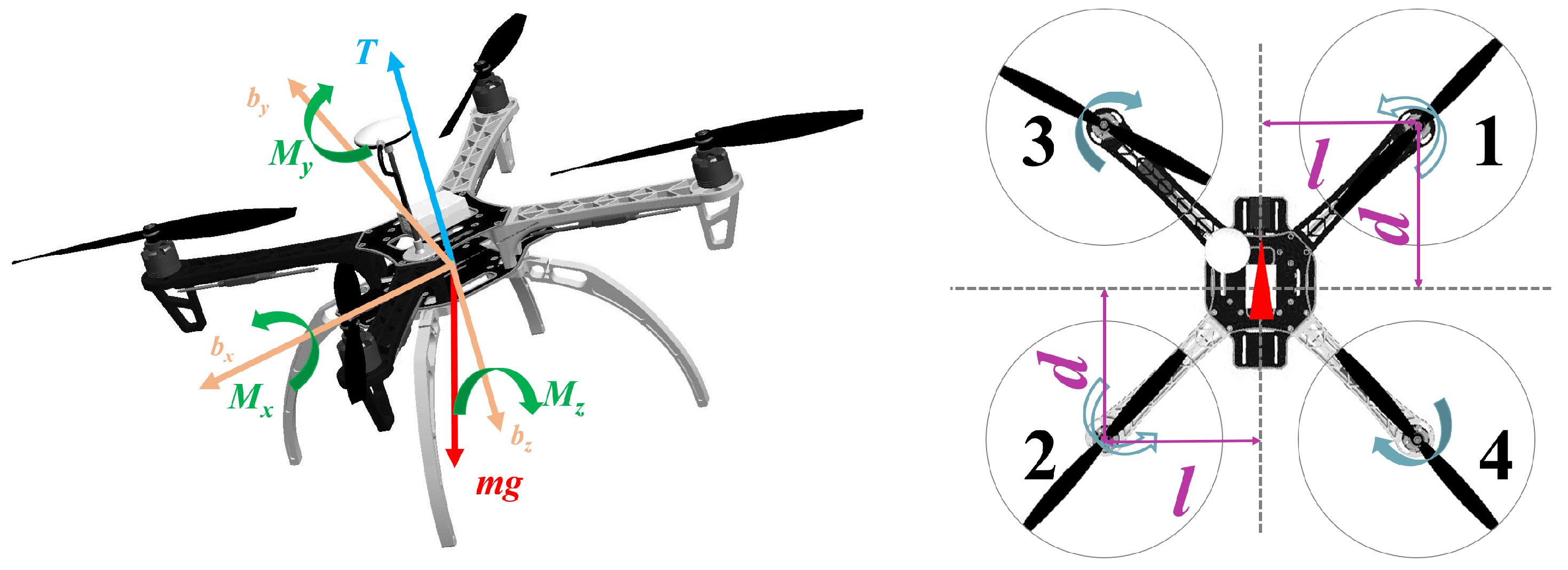
This section primarily discusses the kinematic and dynamic models of quadcopters, serving as the foundation for subsequent research. This paper focuses on a quadcopter with an “X” configuration, as illustrated in Figure 1. Numbers 1–4 represent the propeller number.
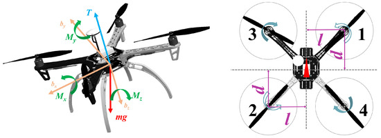
Figure 1.
Aerodynamics and configuration of the quadrotor.
Take to represent the body-fixed reference frame whose direction is indicated by a yellow arrow in Figure 1. T is the total thrust produced by the propellers and is the resultant external torque acting on the three axes of the quadrotor. Define the earth reference frame as . Figure 2 displays the configuration. l and d represent half the distance between the front and rear rotors and between the center and right rotors, respectively.
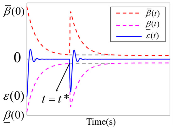
Figure 2.
A schematic of the proposed dynamic event-triggered prescribed performance control.
Assuming the quadrotor is a rigid body, its kinematics and dynamics model [21] can be expressed as follows:
where m is the mass of the quadrotor, g is the gravitational acceleration, and is a unitary vector in . and are the quadrotor’s position and velocity vector in , respectively. is the Euler angles to describe the flight attitude of the quadrotor, including the roll, pitch, and yaw angles. denotes the angular velocity in the . , as shown in (2), is the rotation matrix from to . is a specific matrix and is defined as (3).
where and are abbreviations of and , respectively.
is a specific matrix and is defined as follows:
and in (1) are the total aerodynamic force and moment on the quadrotor, which can be expressed as follows:
where the subscript p represents the aerodynamics generated by the propellers and represents the external disturbance. The composition of and is as follows:
where and () are the thrust and torque of each propeller, respectively.
The goal of quadrotor flight control is to adjust propeller rotation speeds to change T and , then alter the quadrotor’s angular velocity, attitude, velocity, and other states to track the desired commands. To fulfil the afore-mentioned objectives, we adopt the following assumptions to facilitate subsequent research and analysis.
Assumption A1.
The desired state commands are continuous and bounded and the states , , , and in (1) can be obtained through sensor measurements.
Assumption A2.
and , generated by the external disturbance, are bounded, Lipschitz continuous, and can be regarded as slowly changing.
Furthermore, to implement prescribed performance control on the desired quadrotor states, establishing their relationship with the corresponding control signals is essential. The following section will elaborate on this.
3. Dynamic Event-Triggered Prescribed Performance Function
To achieve prescribed control over the targeted performance, Bechlioulis et al. [22] proposed the PPC method, which aims to drive the tracking error to converge to a designed envelope. Building on this foundation, various PPC-based control methods have been developed. However, existing studies still cannot solve the system divergence due to the errors exceeding the bounds caused by variations in task states after the system reaches a steady state. Therefore, we developed a novel performance function based on dynamic event triggering to facilitate envelope adjustments.
3.1. Prescribed Performance Function Design
For a general control system represented as (6), is the system state, is the system output, and is the control input.
The tracking error can be expressed as , where the subscript “” represents the reference command. To design prescribed performance control, first define the error manifold as follows:
where is an adjustable parameter.
To alleviate dependence on the system’s initial state, unlike previous studies, the performance function in this paper is designed in the following form.
where represents the maximum allowable boundary for steady-state errors, while a reflects the desired error convergence time. There are designed parameters, and . represents the dynamic triggering term, and is the compensation factor associated with the command-related performance function. Their definition and composition are provided in Section 3.2.
3.2. Dynamic Event-Triggered Mechanism
In this paper, dynamic event triggering serves to detect whether errors exceed bounds, dynamically adjusting the performance function envelope to maintain effective prescribed performance control. The dynamic event-triggered condition is designed as follows:
where is the designed parameter which represents the permissible safety range of error during a steady state. represent the minimum value between the error and the boundary of the performance function. Equation (9) indicates that the triggering of performance function compensation requires the simultaneous satisfaction of two conditions: the absolute error value exceeds the predetermined safety range, and the minimum distance between the error and the upper and lower bounds of the performance function is outside the range.
The dynamic term in the performance function is designed as follows:
Remark 1.
In (8), , , , and are bounded. constrains the maximum overshoot of the tracking error manifold. represents the maximum range allowed for at a steady state.
Remark 2.
In (10), the first part introduces to extend the boundaries of when the command changes abruptly. The second part is aimed at enlarging the boundaries to ensure that the deviation between and is not less than when is uncontrollable. Both are aimed at preventing error overflow and consequent system divergence.
To ensure that lies within , we define the transformed error before designing the control law. First, the normalized error is defined as follows:
Then, the transformed error can be designed as follows:
Taking the derivative of with respect to time yields, we have,
where
and
Theorem 1.
Supposing that there exists a constant satisfying for , then it follows that .
Proof.
According to and , then .
- For for , there are two cases: (a) and (b) . The case (b) contradicts that .
- For , there have two cases: (a) and (b) . Case (b) contradicts .
□
Therefore, if was valid, then and would exist for .
Figure 2 illustrates the schematic of the proposed dynamic event-triggered prescribed performance control method. The gray dashed line represents the steady-state boundary before performance function adjustment.
Remark 3.
It can be observed that, when the command mutation occurs at , the system error undergoes large-scale variation, exceeding the original steady-state performance function envelope. However, the performance function can dynamically adjust instantly, ensuring envelope error tracking and controlling it within the initially set constraints.
Remark 4.
Compared with the traditional PPC methods introduced in study [23], the proposed performance functions (8) with the dynamic event-triggered mechanism (9) not only quantitatively constrain the state of the quadcopter but also prevent the system divergence caused by error overflow, thus enhancing practicality and flight safety.
4. Controller Design
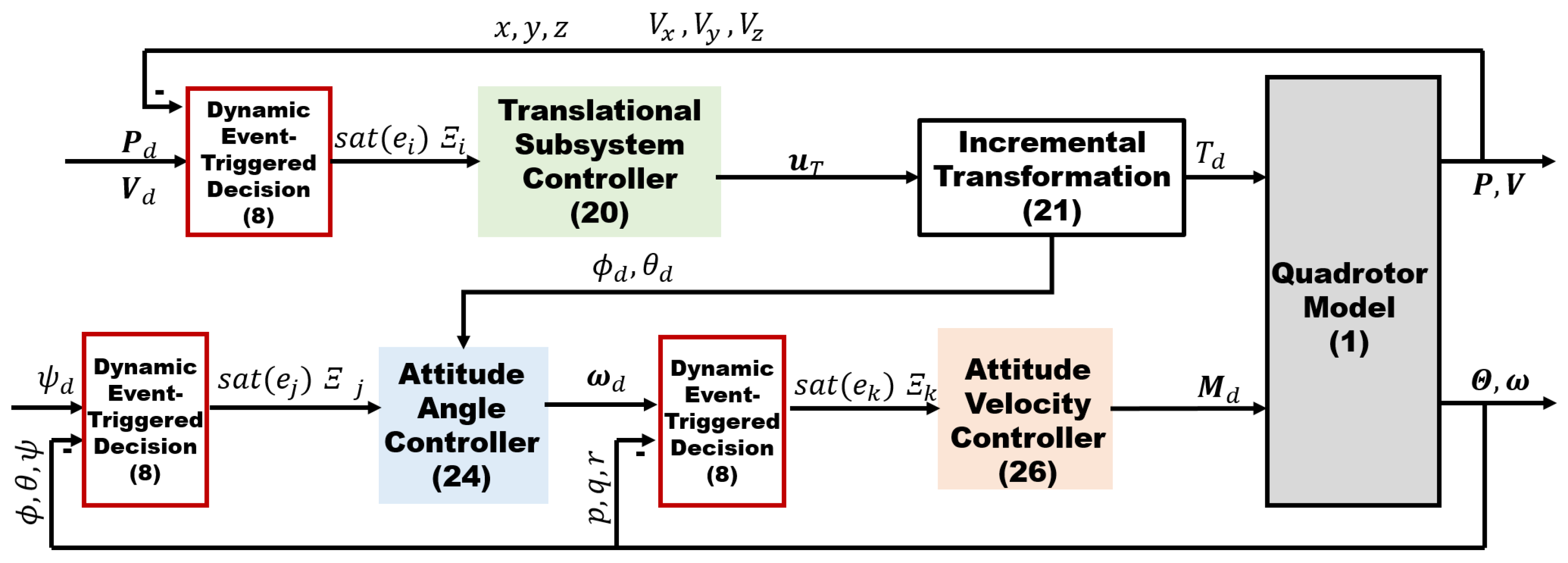
The dynamic event-triggered prescribed performance controller scheme of the quadrotor is shown in Figure 3, and the subsequent sections will provide detailed explanations of the design of each component.
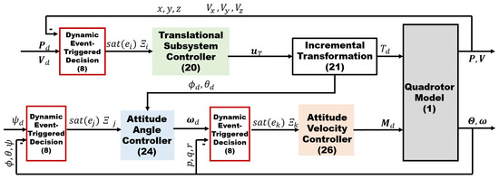
Figure 3.
Dynamic event-triggered prescribed performance control scheme of the quadrotor.
4.1. Translational Subsystem Controller Design
Define the tracking error as , where • represents represents any state variable of the quadrotor in (1). Then, considering Assumptions A1 and A2, the error dynamics of the translation subsystem can be represented as follows:
Considering , the transformation matrix in (16), composed of trigonometric functions of the attitude angles, as shown in (2), can be obtained using the sum and difference identities of trigonometric functions as follows:
With reference to (7), define as the error manifold of the translational subsystem, where . The performance function of the translational subsystem in this paper is designed as follows:
where , .
Combining the definition of a normalized error in this paper, the control law for the translational subsystem can be derived as follows:
where is a positive definite control gain matrix, and are expressed by (24) and (25).
in (23) essentially represents the linear acceleration command. Generally, based on force equilibrium, the desired attitude angles and total thrust of a quadrotor can be obtained by applying Newton’s second law to the linear acceleration commands. However, this neglects the influence of air resistance, leading to errors in command derivation. Based on an incremental nonlinear dynamic inversion method, the authors of [24] established mapping between quadcopter linear acceleration and horizontal attitude angles, as shown in (26), demonstrating a significant enhancement in the accuracy of attitude angle commands.
where T is the total thrust. Variables with subscript d represent desired commands, while the remaining state variables represent measurements from sensors at the current time. Based on (26), considering the definition of , then based on the translational subsystem controller, the desired total thrust, roll, and pitch angle of the quadrotor can be obtained as follows:
where
4.2. Rotational Subsystem Controller Design
Similar to the translational subsystem controller design, the performance function for the attitude control of the quadrotor is selected as (29).
Define the output of the quadrotor attitude controller as ; this means the virtual desired angular velocity, which can be expressed in (30).
where is a positive definite control gain matrix and can be expressed by (31).
where .
For angular velocity control, the performance functions are selected as (32) and the control signal can be deduced as (33).
where is a positive definite control gain matrix and can be expressed by (34).
where .
Therefore, the desired moment of the quadrotor can be obtained as .
5. Stability Analysis
To facilitate derivation, combining (1) and (6), rewrite the quadrotor angular velocity subsystem as follows:
where is an unknown non-affine Lipschitz continuous function; is the external disturbance.
According to [18], there exist continuous functions, , , , and , and unknown constants, and , , which make the following inequalities hold.
Theorem 2.
Suppose that both and are bounded. By combining the quadrotor translational and rotational subsystem control outputs, (23), (30), and (33), the following properties can be ensured:
- For , exists with and .
- All the state variables in (1) for quadcopters are bounded.
Proof.
Based on (36) and the extreme value theory, there exist continuous functions, and , such that the following inequalities hold.
where are unknown constants.
Then, rewrite as follows:
with
where and , factors , .
Then, define the normalized error for all states of the quadrotor as , whose derivative is defined as follows:
where .
Define , which constrains that , and there exists a maximal solution that fulfils for [18]. Thus, set a constant and , then it can be obtained that .
Step 1.
Differentiate the error manifold of the translational subsystem as follows:
where and .
Define the Lyapunov function candidate , where and are a positive definite diagonal matrix. Take the derivative of with respect to time as follows:
where and . Choose and submit (23) into (43); we thus have
where .
Consider the following boundedness condition:
- , , , and , are bounded;
- , , and are bounded;
- According to extreme value theory, and for , there is a constant that satisfies for .
Based on Young’s inequality, together with , it can be deduced that
where . Because is positive definite, then we have
According to the boundary theory of nonlinear systems based on definiteness [25], it can be obtained that for , where
Therefore, and , are bounded and for .
Step 2.
Differentiate with respect to time as follows:
where .
Define the Lyapunov function candidate , where and represent a positive definite diagonal matrix. Take the derivative of as follows:
where , . Choosing and taking (30) into (51), we have
Consider the following boundedness conditions:
- and , are bounded;
- and are bounded by the former step;
- and are bounded for .
Because and are both positive diagonal matrixes, it can be deduced as follows:
Thus, we can conclude that for with . Thus, and are bounded and for .
Step 3.
Differentiate , respect to time as follows:
where .
Define the Lyapunov function candidate , then its derivative with respect to time can be represented as follows:
Consider the following boundedness conditions:
- and , are bounded;
- and are bounded by the former step;
- Based on the extreme value theory, and are bounded for and there exists a constant that satisfies
According to the above conditions, it can be obtained as follows:
After that, it can be concluded that for with . Therefore, we can obtain that and , are bounded and for .
Step 4.
According to the setting that for , where
Thus, it can be assumed that and , and it can be demonstrated that there exists a time instant satisfying [25]. It is obvious that such a deduction is contradictory to .
Hence, it can be concluded that all states of the closed-loop quadrotor based on the proposed dynamic event-triggered PPC remain bounded and . Furthermore, we can obtain the following conclusion:
□
Henceforth, all proofs are complete.
6. Simulation and Discussion
In order to verify the effectiveness of the proposed method, we provide quadrotor aggressive flight simulations. The parameters of the quadrotor model and DETPPC controllers designed are as shown in Table 1. At the same time, the measurement noise of the sensor is taken into account.

Table 1.
The structural parameters and DETPPC controller parameters of the quadcopter.
The performance functions of each subsystem are, respectively, designed as (22), (29), and (32), the parameters of which are displayed in Table 1.
This paper selects two controllers for comparison: (1) a traditional prescribed performance controller (TPPC) without dynamic event-triggering, with controller parameters consistent with DETPPC; (2) a Cascade PID controller (P-PID), with parameters set according to Wang [26].
Example 1.
To verify the improvement in the transient performance of the proposed method for quadrotors facing abrupt commands, this example conducts a simulation of an attitude control under abrupt mutations. The reference attitude commands (), as defined in (60), are employed for attitude control simulation. in (60) denotes that the roll and pitch attitude angles of the quadrotor were initially subjected to sinusoidal commands. However, at the 3rd and 9th seconds, due to specific flight requirements, their values experienced abrupt changes and were maintained for 3 s each. The initial attitude and angular velocity of the quadrotor are set to and .
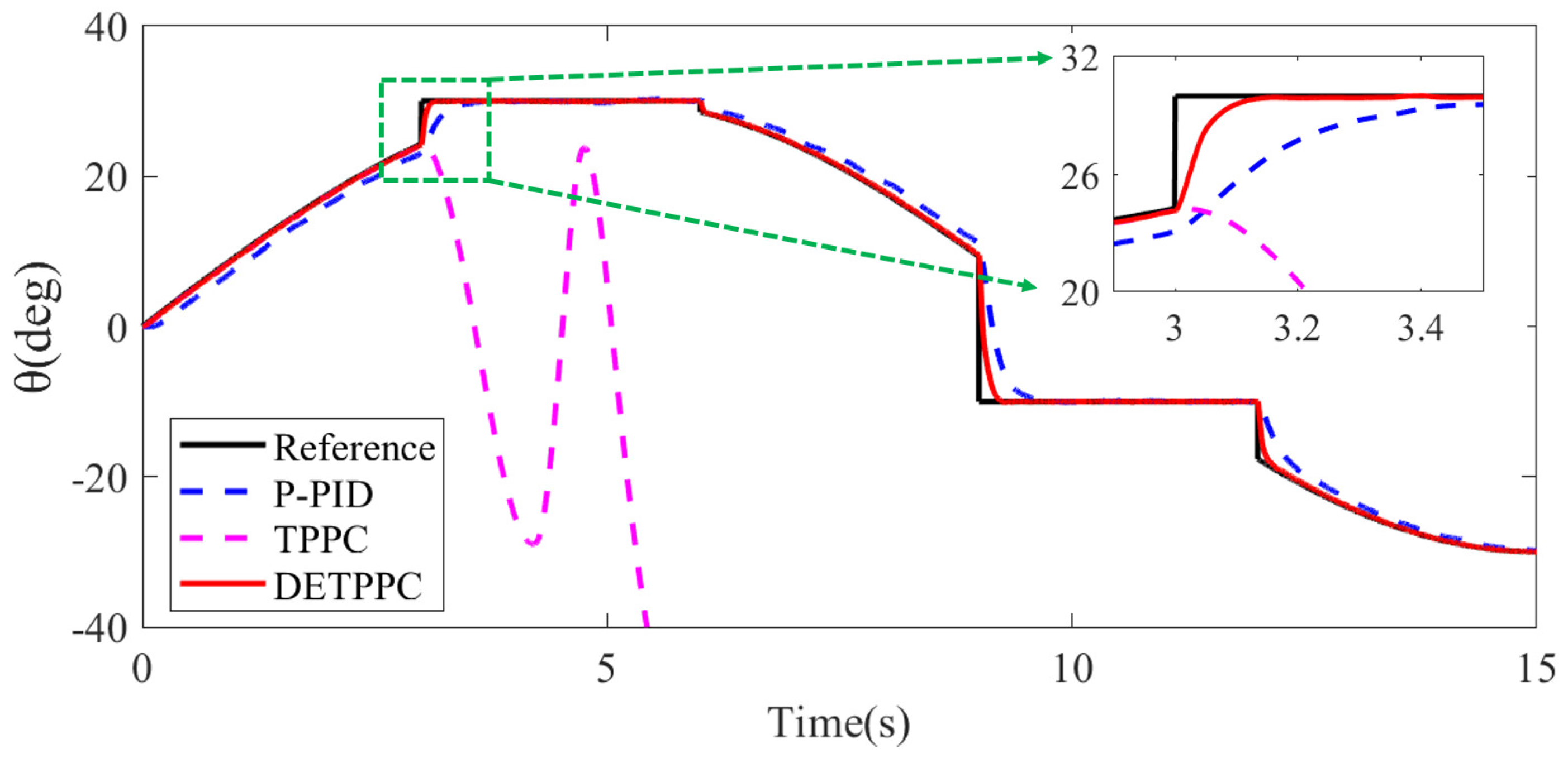
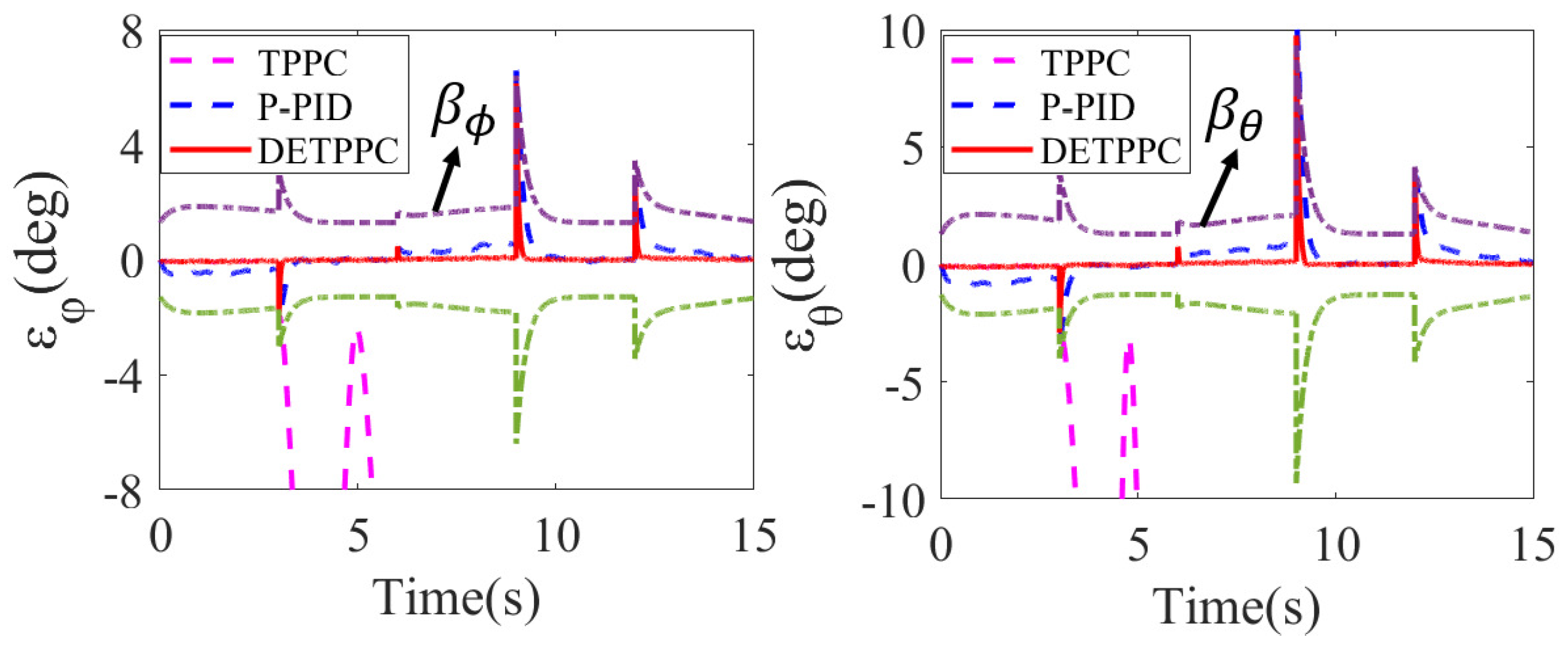
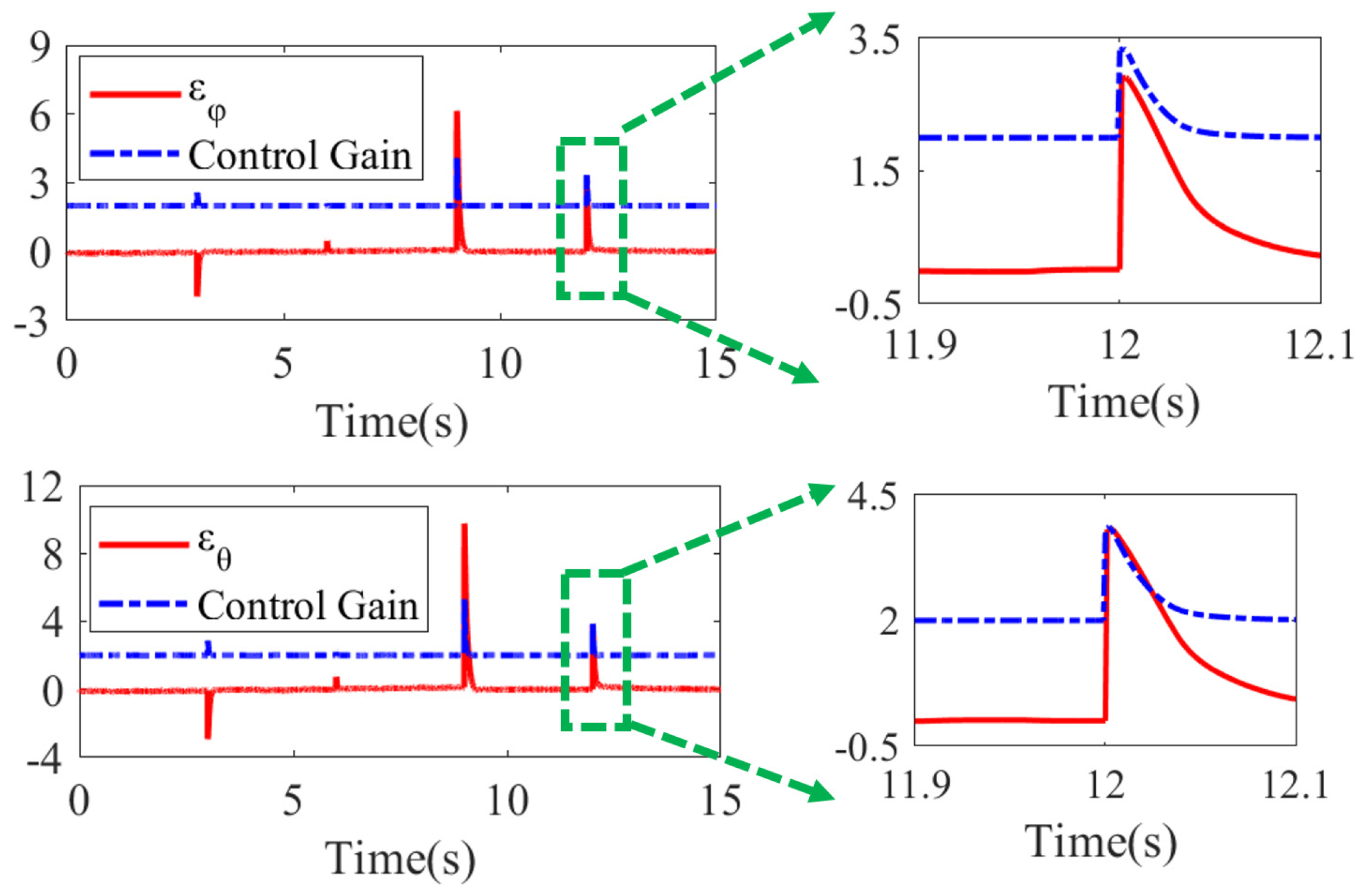
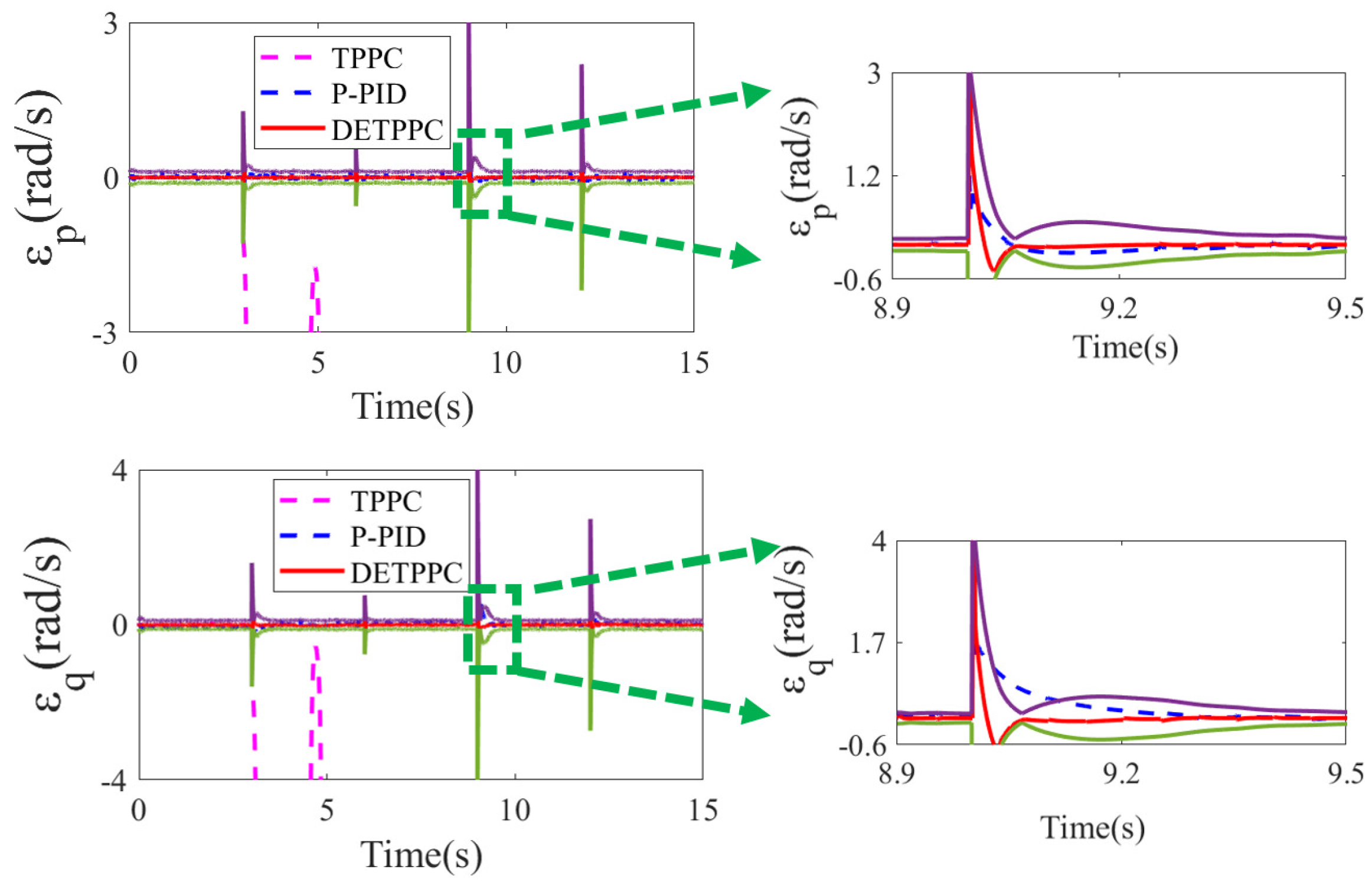
Figure 4 and Figure 5 present the tracking results. Due to the absence of performance function compensation based on dynamic event triggering, the TPPC controller diverges when the command abruptly changes at the third second. In comparison with the P-PID method, the DETPPC controller in this study demonstrates faster response and convergence rates, as well as smaller tracking errors. Figure 6 illustrates a comparison of the convergence of . The purple and green dashed lines represent the proposed DETPPC performance function. The TPPC method encounters an error overshoot at the third second, which is the cause of control divergence. The proposed DETPPC controller demonstrates faster and more stable error convergence than the P-PID controller. In Figure 7, DETPPC’s control gain dynamically adjusts based on variations. This accounts for DETPPC’s faster convergence and response speed compared to traditional cascade PID methods when handling abrupt commands.
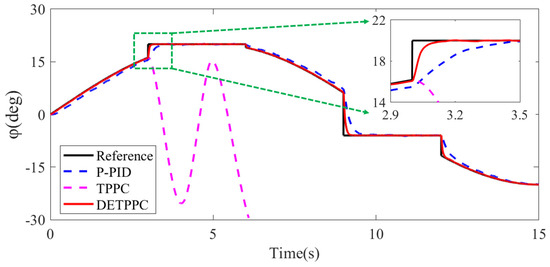
Figure 4.
The tracking results of angle.
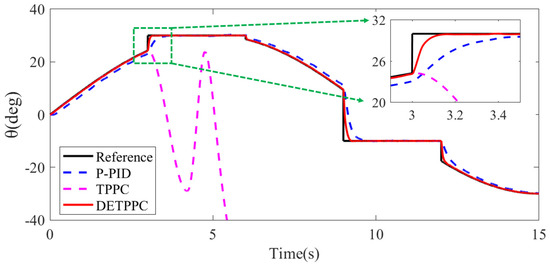
Figure 5.
The tracking results of angle.
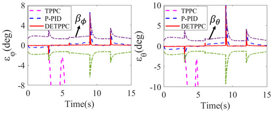
Figure 6.
Comparision of the tracking error of attitude angle.
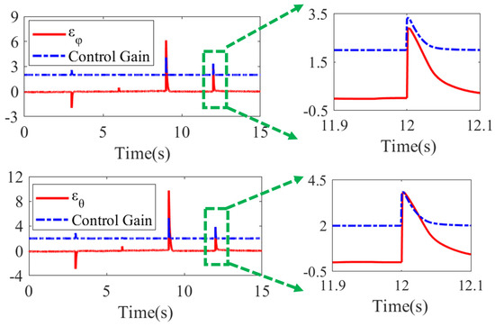
Figure 7.
The control gain of DETPPC varies with the tracking error.
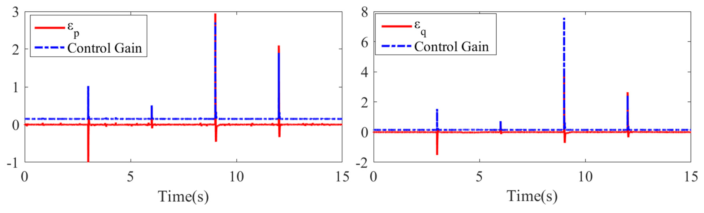
Figure 8 and Figure 9, respectively, depict and the variation of DETPPC control gain with the angular rate tracking errors. Besides the divergence seen in the TPPC method during command mutations, it is evident that, for pitch angular velocity control, the DETPPC controller also shows faster and more stable convergence. Moreover, the tracking error based on the P-PID method occasionally surpasses the expected performance boundaries. For roll angular velocity, DETPPC and P-PID controllers perform similarly, likely due to the small reference command for roll angle.
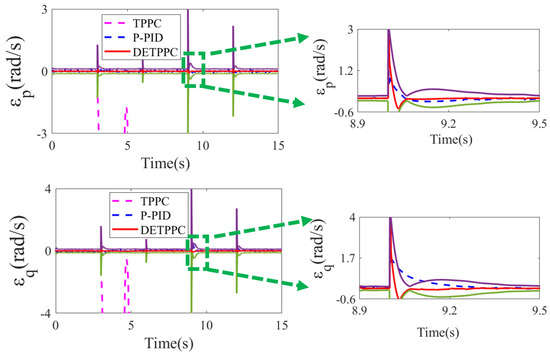
Figure 8.
Comparision of the tracking error of angular velocity.
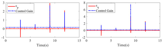
Figure 9.
The control gain of DETPPC varies with the angular velocity tracking error.
To sum up, the proposed DETPPC method resolves the divergence problem faced by traditional PPC when confronted with command mutations, while also achieving superior transient performance through tailored constraint design for specified state variables.
Example 2.
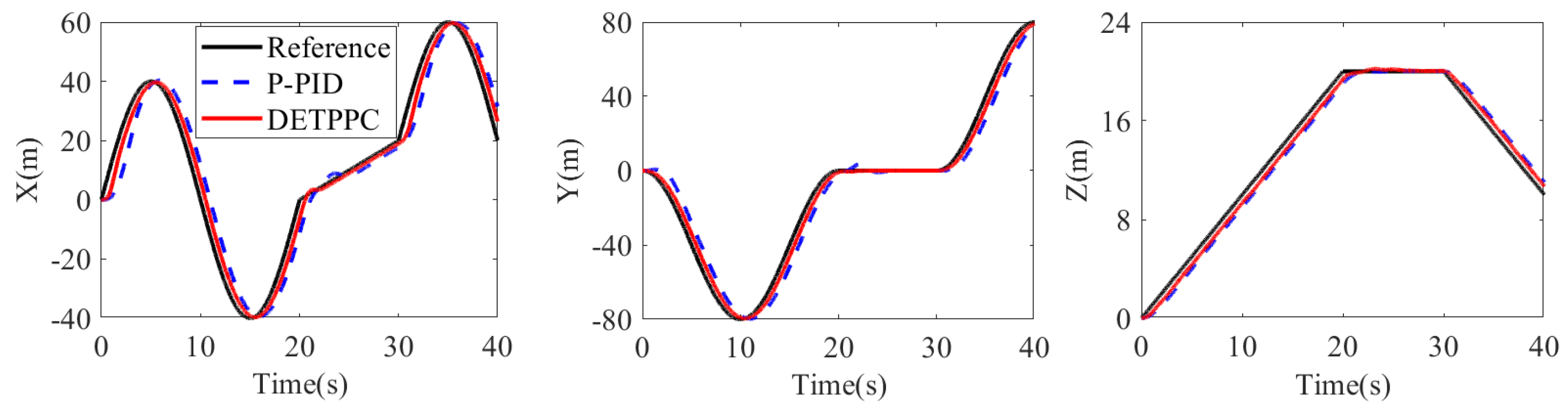
To further validate the afore-mentioned conclusions, this example provides a simulation of agile trajectory tracking for a quadrotor with abrupt command. As errors exceeding performance function boundaries lead to system divergence, the traditional PPC method is not included as a comparison in this simulation. The reference trajectory in this example is a three-dimensional helix, as shown in (61). External disturbances are encountered at the tenth second, persisting for two seconds. Additionally, trajectory command changes occur at the twentieth and thirtieth seconds, respectively. The initial position of the quadcopter is set to .
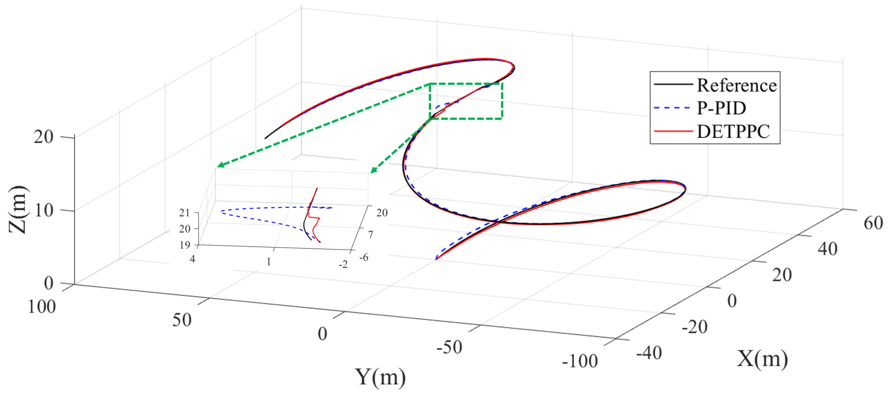
Figure 10 and Figure 11 present the results of trajectory tracking and position control in three directions, respectively. It can be observed that the DETPPC method enables more accurate trajectory tracking, which is particularly evident during the command mutation at 20 s, where the proposed DETPPC method exhibits reduced overshoot and faster position convergence. Take the root-mean-square (RMS, ) values of the tracking errors, as shown in Table 2, to quantitatively evaluate the controller effectiveness. The results demonstrate that the trajectory tracking RMS of the proposed method is only 31% of that of the traditional approach.
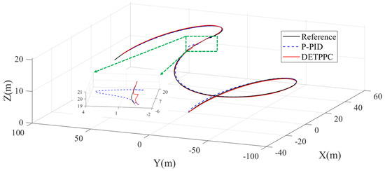
Figure 10.
The trajectory tracking results in comparison.
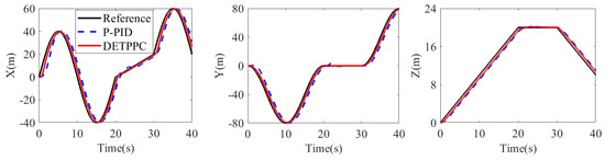
Figure 11.
The results of position control in three directions.
Table 2.
RMS of the trajectory tracking errors.
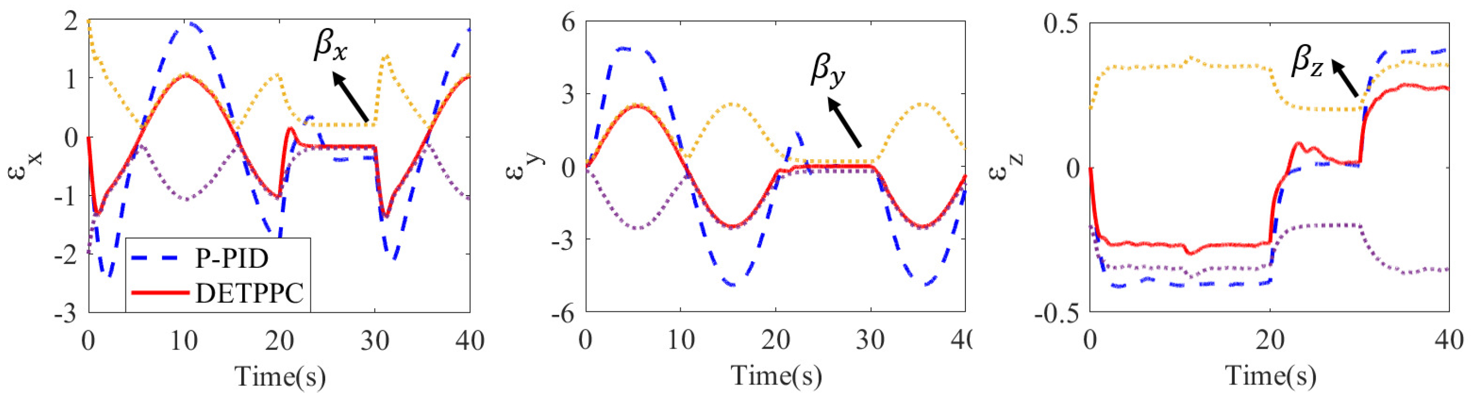
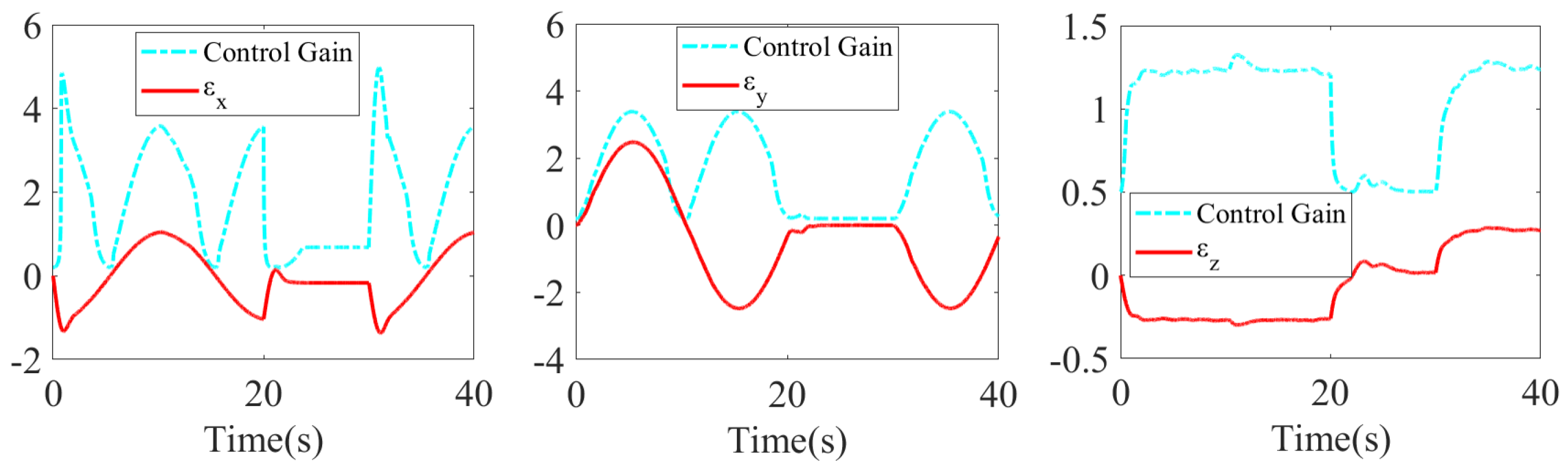
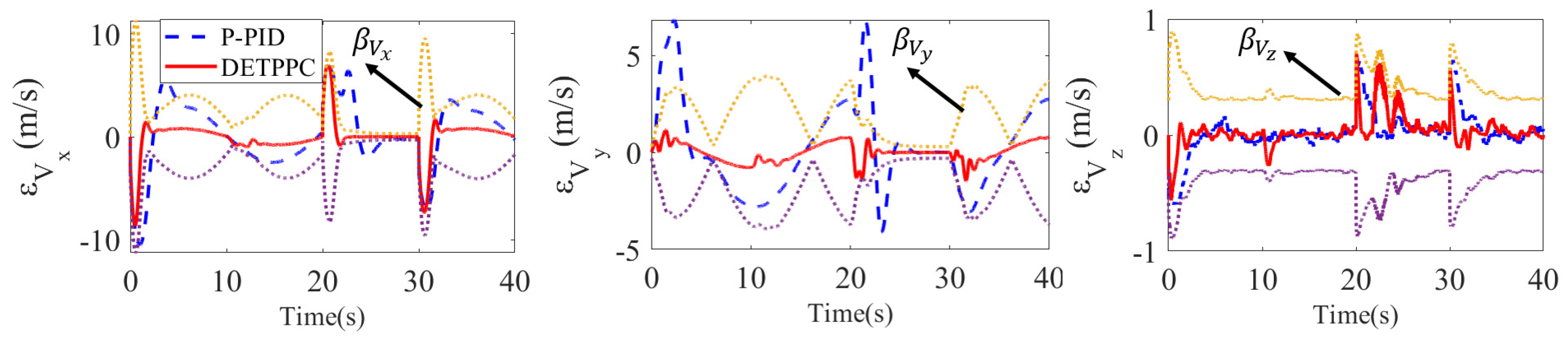
The convergence of for the quadrotor is illustrated in Figure 12. By imposing performance constraints, DETPPC achieves faster convergence of tracking errors with smaller overshoots through automatic adjustment of control gains, as depicted in Figure 13. In comparison, the position control errors of the P-PID method notably deviate from the desired criteria, especially in the horizontal direction. The position tracking error of the proposed method is only 50% that of the P-PID controller in the horizontal direction, and 75% in the vertical direction. Similarly, the velocity control of the quadcopter in three axes shows the same trend. As depicted in Figure 14, DETPPC facilitates quicker convergence of velocity control, particularly with reduced fluctuations during command changes.
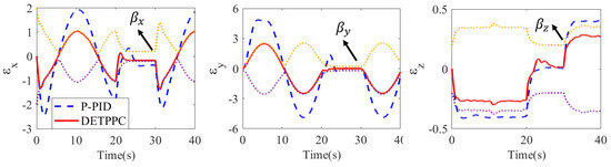
Figure 12.
The convergence of position tracking errors.
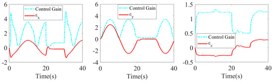
Figure 13.
The variation of position control gains with tracking errors.

Figure 14.
The convergence of velocity control errors.
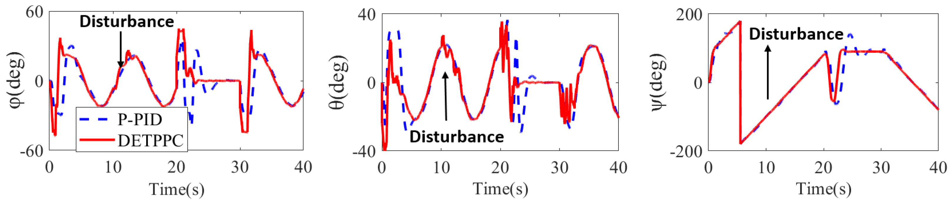
Figure 15, Figure 16 and Figure 17 demonstrate the control comparison of attitude angles and angular rates. For the desired trajectory in (61), the quadrotor’s attitude angles reached 40 degrees. Furthermore, the proposed DETPPC method reaches peak attitude angles nearly 2 s faster than the P-PID controller. Figure 15 demonstrates that, with DERPPC, the quadrotor achieves more agile attitude control. Additionally, in Figure 16, during the 10–12 s period of external disturbance, the proposed method demonstrates rapid attitude convergence, while the P-PID controller exhibits larger and longer fluctuations, especially in roll and pitch angles. in Figure 17 also reflects the same conclusion.
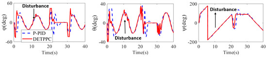
Figure 15.
The response of the quadrotor’s attitude angles.
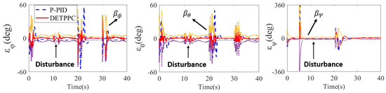
Figure 16.
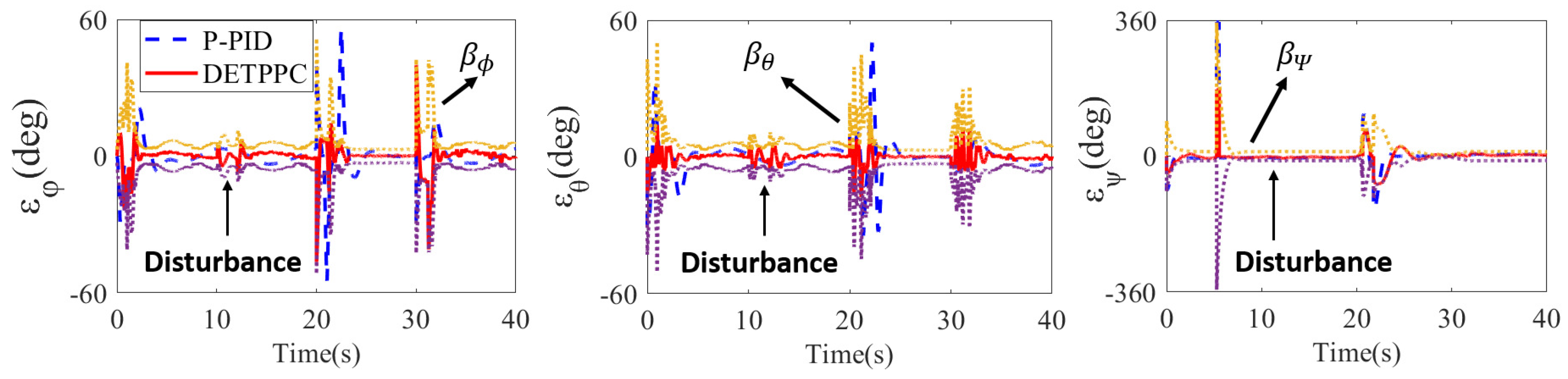
The convergence of attitude angle control errors.
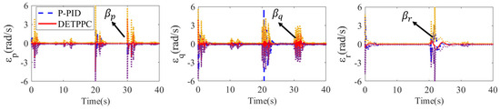
Figure 17.
The convergence of angular rate control errors.
7. Conclusions
Originating from the demands of quadrotor aggressive flight for maneuverability and transient performance, this paper aims to address the control divergence caused by command mutations in existing PPC methods. Through designing a dynamic event-triggered mechanism, and using the direction of error variation and its distance from the envelope of the performance function as triggering criteria, the performance function can be autonomously compensated. Based on this, the performance function was redesigned, and robust prescribed performance controllers for the quadrotor’s translational and rotational subsystems were, respectively, designed. Moreover, a stability analysis of the controller was conducted based on Lyapunov functions. Finally, simulations were conducted to evaluate attitude control and aggressive trajectory tracking under command mutations and external disturbances. The results indicate that the proposed method resolves the divergence of traditional PPC controllers under abrupt command changes, enhancing the algorithm’s robustness. Additionally, compared to the cascaded PID method, the proposed DETPPC controller exhibits faster response and convergence speeds, along with reduced oscillations, in trajectory tracking simulations under sudden command changes. Ultimately, it achieves an RMS trajectory tracking error that is only 31% of the control group. We believe that this work can provide a reference for practical applications, while also indicating areas that require further exploration. It is worth noting that our proposed method has shown that control gains vary with error convergence. Hence, energy consumption during application needs attention, even potentially control saturation. This provides us with further ideas for our future research and for enhancing the practicality of the algorithm.
Author Contributions
Conceptualization, Z.W. and J.Y.; methodology, Z.W.; software, Z.W. and T.S.; validation, Z.W. and J.Y.; investigation, resources and data curation, Z.W. and J.Y.; writing—original draft preparation, Z.W.; writing—review and editing, J.Y. and T.S.; visualization, Z.W.; supervision, J.Y.; project administration, T.S. All authors have read and agreed to the published version of the manuscript.
Funding
This research was funded by the China Postdoctoral Science Foundation (2023M731913) and Civilian Aircraft Research (MJG5-1N21).
Data Availability Statement
The data presented in this study are available on request from the corresponding author.
Conflicts of Interest
The authors declare no conflict of interest.
References
- Fan, B.; Li, Y.; Zhang, R.; Fu, Q. Review on the technological development and application of UAV systems. Chin. J. Electron. 2020, 29, 199–207. [Google Scholar] [CrossRef]
- Zhen, Z.; Jiang, J.; Sun, S.; Wang, B. Cooperative Control and Decision of UAV Swarm Operations; National Defense Industry Press: Beijing, China, 2022. [Google Scholar]
- Liu, Z.; Wang, X.; Shen, L.; Zhao, S.; Cong, Y.; Li, J.; Yin, D.; Jia, S.; Xiang, X. Mission-oriented miniature fixed-wing UAV swarms: A multilayered and distributed architecture. IEEE Trans. Syst. Man Cybern. Syst. 2020, 52, 1588–1602. [Google Scholar] [CrossRef]
- Bry, A.; Richter, C.; Bachrach, A.; Roy, N. Aggressive flight of fixed-wing and quadrotor aircraft in dense indoor environments. Int. J. Robot. Res. 2015, 34, 969–1002. [Google Scholar] [CrossRef]
- Jia, J.; Guo, K.; Yu, X.; Guo, L.; Xie, L. Agile flight control under multiple disturbances for quadrotor: Algorithms and evaluation. IEEE Trans. Aerosp. Electron. Syst. 2022, 58, 3049–3062. [Google Scholar] [CrossRef]
- Belmouhoub, A.; Medjmadj, S.; Bouzid, Y.; Derrouaoui, S.; Guiatni, M. Enhanced backstepping control for an unconventional quadrotor under external disturbances. Aeronaut. J. 2023, 127, 627–650. [Google Scholar] [CrossRef]
- Labbadi, M.; Boudaraia, K.; Elakkary, A.; Djemai, M.; Cherkaoui, M. A continuous nonlinear sliding mode control with fractional operators for quadrotor UAV systems in the presence of disturbances. J. Aerosp. Eng. 2022, 35, 04021122. [Google Scholar] [CrossRef]
- Wang, J.; Alattas, K.A.; Bouteraa, Y.; Mofid, O.; Mobayen, S. Adaptive finite-time backstepping control tracker for quadrotor UAV with model uncertainty and external disturbance. Aerosp. Sci. Technol. 2023, 133, 108088. [Google Scholar] [CrossRef]
- Jabeur, C.B.; Seddik, H. Optimized neural networks-PID controller with wind rejection strategy for a Quad-Rotor. J. Robot. Control JRC 2022, 3, 62–72. [Google Scholar] [CrossRef]
- Wang, J.; Zhu, B.; Zheng, Z. Robust Adaptive Control for a Quadrotor UAV with Uncertain Aerodynamic Parameters. IEEE Trans. Aerosp. Electron. Syst. 2023, 59, 8313–8326. [Google Scholar] [CrossRef]
- Shao, X.; Xu, L.; Zhang, W. Quantized control capable of appointed-time performances for quadrotor attitude tracking: Experimental validation. IEEE Trans. Ind. Electron. 2021, 69, 5100–5110. [Google Scholar] [CrossRef]
- Cui, G.; Yang, W.; Yu, J.; Li, Z.; Tao, C. Fixed-time prescribed performance adaptive trajectory tracking control for a QUAV. IEEE Trans. Circuits Syst. II Express Briefs 2021, 69, 494–498. [Google Scholar] [CrossRef]
- Jia, F.; Wang, X.; Zhou, X. Robust adaptive prescribed performance control for a class of nonlinear pure-feedback systems. Int. J. Robust Nonlinear Control 2019, 29, 3971–3987. [Google Scholar] [CrossRef]
- Verginis, C.K.; Bechlioulis, C.P.; Dimarogonas, D.V.; Kyriakopoulos, K.J. Robust distributed control protocols for large vehicular platoons with prescribed transient and steady-state performance. IEEE Trans. Control Syst. Technol. 2017, 26, 299–304. [Google Scholar] [CrossRef]
- Bu, X.; Wu, X.; Zhu, F.; Huang, J.; Ma, Z.; Zhang, R. Novel prescribed performance neural control of a flexible air-breathing hypersonic vehicle with unknown initial errors. ISA Trans. 2015, 59, 149–159. [Google Scholar] [CrossRef] [PubMed]
- Bu, X.; Xiao, Y. Prescribed performance-based low-computational cost fuzzy control of a hypersonic vehicle using non-affine models. Adv. Mech. Eng. 2018, 10, 1687814018757261. [Google Scholar] [CrossRef]
- Xu, J.; Wang, L.; Liu, Y.; Xue, H. Finite-time prescribed performance optimal attitude control for quadrotor UAV. Appl. Math. Model. 2023, 120, 752–768. [Google Scholar] [CrossRef]
- Wang, Y.; Hu, J. Robust control for a quadrotor aircraft with small overshoot and high-precision position tracking performance. J. Frankl. Inst. 2020, 357, 13386–13409. [Google Scholar] [CrossRef]
- Wang, Y.; Hu, J. Improved prescribed performance control for air-breathing hypersonic vehicles with unknown deadzone input nonlinearity. ISA Trans. 2018, 79, 95–107. [Google Scholar] [CrossRef]
- Wang, Y.; Hu, J.; Li, J.; Liu, B. Improved prescribed performance control for nonaffine pure-feedback systems with input saturation. Int. J. Robust Nonlinear Control 2019, 29, 1769–1788. [Google Scholar] [CrossRef]
- Padfield, G.D. Helicopter Flight Dynamics: Including a Treatment of Tiltrotor Aircraft; John Wiley & Sons: Hoboken, NJ, USA, 2018. [Google Scholar]
- Bechlioulis, C.P.; Rovithakis, G.A. A low-complexity global approximation-free control scheme with prescribed performance for unknown pure feedback systems. Automatica 2014, 50, 1217–1226. [Google Scholar] [CrossRef]
- Bu, X. Prescribed performance control approaches, applications and challenges: A comprehensive survey. Asian J. Control 2023, 25, 241–261. [Google Scholar] [CrossRef]
- Pfeifle, O.; Fichter, W. Cascaded incremental nonlinear dynamic inversion for three-dimensional spline-tracking with wind compensation. J. Guid. Control Dyn. 2021, 44, 1559–1571. [Google Scholar] [CrossRef]
- Sastry, S. Nonlinear Systems: Analysis, Stability, and Control; Springer Science & Business Media: Berlin/Heidelberg, Germany, 2013; Volume 10. [Google Scholar]
- Wang, L. PID Control System Design and Automatic Tuning Using MATLAB/Simulink; John Wiley & Sons: Hoboken, NJ, USA, 2020. [Google Scholar]


Disclaimer/Publisher’s Note: The statements, opinions and data contained in all publications are solely those of the individual author(s) and contributor(s) and not of MDPI and/or the editor(s). MDPI and/or the editor(s) disclaim responsibility for any injury to people or property resulting from any ideas, methods, instructions or products referred to in the content. |
© 2024 by the authors. Licensee MDPI, Basel, Switzerland. This article is an open access article distributed under the terms and conditions of the Creative Commons Attribution (CC BY) license (https://creativecommons.org/licenses/by/4.0/).