UAV Control Based on Pattern Recognition in Aquaculture Application

Abstract

This study proposes a drone application for the net cage aquaculture industry. A visual control structure is applied to the drone to obtain water-quality information surrounding the net cages. This study integrates a hexacopter, camera, onboard computer, flight control board, servo motor, and global positioning system’s auto-cruise function to adjust the drone position and control the servo motor retractable sensor to reach the desired target at an accurate location. In object identification, a deep learning neural network is used to identify the net cages. An onboard computer calculates the horizontal distance between the drone and the net cage. A “You only look once” (YOLO) neural network is used to detect the net cage images. Considering the hardware calculation speed and ability, an onboard computer is applied to process the flight control board and control the drone. In the mission, an aerial camera detects targets (net cage) and provides visual information to the drone for the target approaching control process. After executing the water-quality measurement, the drone will end the mission and return to the base. This study modifies the architecture of YOLO, compares it with the original model, and then finds a proper architecture for this mission. This study aims to assist cage aquaculture operators by using drones to measure water quality, which can reduce aquaculture’s labor costs.

1. Introduction

In recent years, unmanned aerial vehicles (UAVs) have been widely used in movies, aerial films, inspection, military, and fishing. Multi-rotor aircraft were also developed with different mission requirements. This study mainly considered the flight speed, endurance, and maximum takeoff weight using a hexacopter. Most of the time, the UAV will fly out of sight, making it difficult for the operator to control it. In this study, we combined visual image identification, which is widely used in face recognition and license plate recognition. However, traditional image recognition is unable to identify complex targets. Thus, the deep learning neural network is used in UAVs to recognize different targets. One can apply drones to more applications by combining visual recognition and UAVs. There are many types of UAVs, most of which can be classified into two categories: fixed-wing aircraft and multi-rotor aircraft. The advantages of fixed-wing aircraft are high speed, high flight efficiency, long suspension time, and height, which is much higher than traditional drones. The disadvantage is that a particular flight speed must be maintained to allow the aircraft to sustain proper lift. The takeoff and landing location also limits it, and the maneuverability is also low. Compared to fixed-wing aircraft, multi-rotor aircraft can take off and land vertically, have high maneuverability, and perform fixed-point tasks. The shortcomings of the multi-rotor aircraft are short flying range, low flying height, low speed, and less load. After considering the flight mission’s load and stability, this study selected a hexacopter as the carrier. The hexacopter can hover at the same height, take off, and land vertically, and its ability to move in three-dimensional space is very good. It can also be equipped with a global positioning system (GPS) and an inertial navigation system (INS) to increase the stability and accuracy of the UAV’s autonomous flight navigation.

The development of the six-axis aircraft began in France in 1970. D.K. Tiep [1] used fuzzy proportional-derivative (PD) control to stabilize UAV flight. N.M. Raharja [2] used fuzzy control to stabilize the drone hover. These studies make UAVs more stable and reliable. P. Pounds used a commercially available electric motor to control the rotation speed [3], which also made the application of drones go further. Several fuzzy control methods have been applied. In recent years, more and more drones have integrated image processing technology. M.A. Olivares-Méndez improved the stability of the landing by using cameras. Moving targets can also be tracked in [4]. In 2012, Alex Krizhevsky proposed an image-learning algorithm that made Alexnet the first image deep learning in recent years [5]. The difference between deep learning image recognition and traditional image recognition is that deep learning image recognition can recognize more complex objects. In 2016, J. Redmon proposed the “You only look once” (YOLO) algorithm, which uses first-stage object recognition [6]. YOLOv2 was proposed in 2017 [7]. In addition to faster recognition, it has more accurate recognition than YOLO, which solves the problem of predicting dense targets. The YOLOv3 used in this study was proposed in 2018 [8]. Although it is not faster than YOLOv2 in recognition speed, it is much better than YOLOv2 in accuracy. The quicker and more accurate algorithm means it can be deployed on faster vehicles. Currently, more versions of YOLO are being presented, such as YOLOv7 and YOLOv8 [9,10]. These models can provide higher accuracy, but the structures are more complex and take more computing time, which is unsuitable for this study. In this study, we modified YOLOv3 to fit the net cage aquaculture task’s time requirement and keep recognition errors low.

Collecting data on water quality, pollutants, temperature, and fish behavior in aquaculture farms requires tremendous labor and effort. UAVs provide greater efficiency and accuracy in executing aquaculture farm management and surveillance operations. In 2022, N.A. Ubina and S.C. Cheng provided an overview of the capabilities of unmanned systems to monitor and manage aquaculture farms that support precision aquaculture using the Internet of Things [11]. Traditional fish weight measurement is time-consuming and can stress the fish. Image analysis has been applied to solve these problems. In [12], the authors used UAV combined with image analysis to obtain more comprehensive area images and evaluate the weight of red tilapia in a fish cage farm. A low-cost, cloud-based autonomous drone system was presented to survey and monitor aquaculture sites [13]. To perform aquaculture surveillance tasks, they applied computer vision and various deep learning recognition models to achieve scalability and added functionality. The aquaculture cloud enables the drone to execute its surveillance task more efficiently with increased navigation time. The mobile drone navigation app can send surveillance alerts and reports to users [13].

Some researchers have studied the application of UAV remote sensing technology in water quality monitoring. Cheng et al. [14] used UAVs to quantitatively map the Chl-a distribution of surface water in coastal waters from low altitudes. Liu et al. [15] constructed an inverse model based on UAV multispectral images for three water quality parameters: total phosphorus, suspended solids, and turbidity. McEliece et al. [16] applied UAV multispectral imagery to inverse chlorophyll-a and turbidity in nearshore water bodies. Moreover, Matsui et al. [17] used UAV remote sensing imagery combined with neural networks to compensate for the lack of resolution of satellite remote sensing imagery to achieve high-resolution monitoring of suspended sediment concentrations. Zhang et al. [18] evaluated the water quality of the cultured water in the Beibu Gulf of Guangxi and obtained spectral reflectance by UAV with multispectral image sensors. Although the results of these studies were satisfactory, the estimated data were not 100% accurate. None of them used physical sensors to measure the water quality to get accurate values.

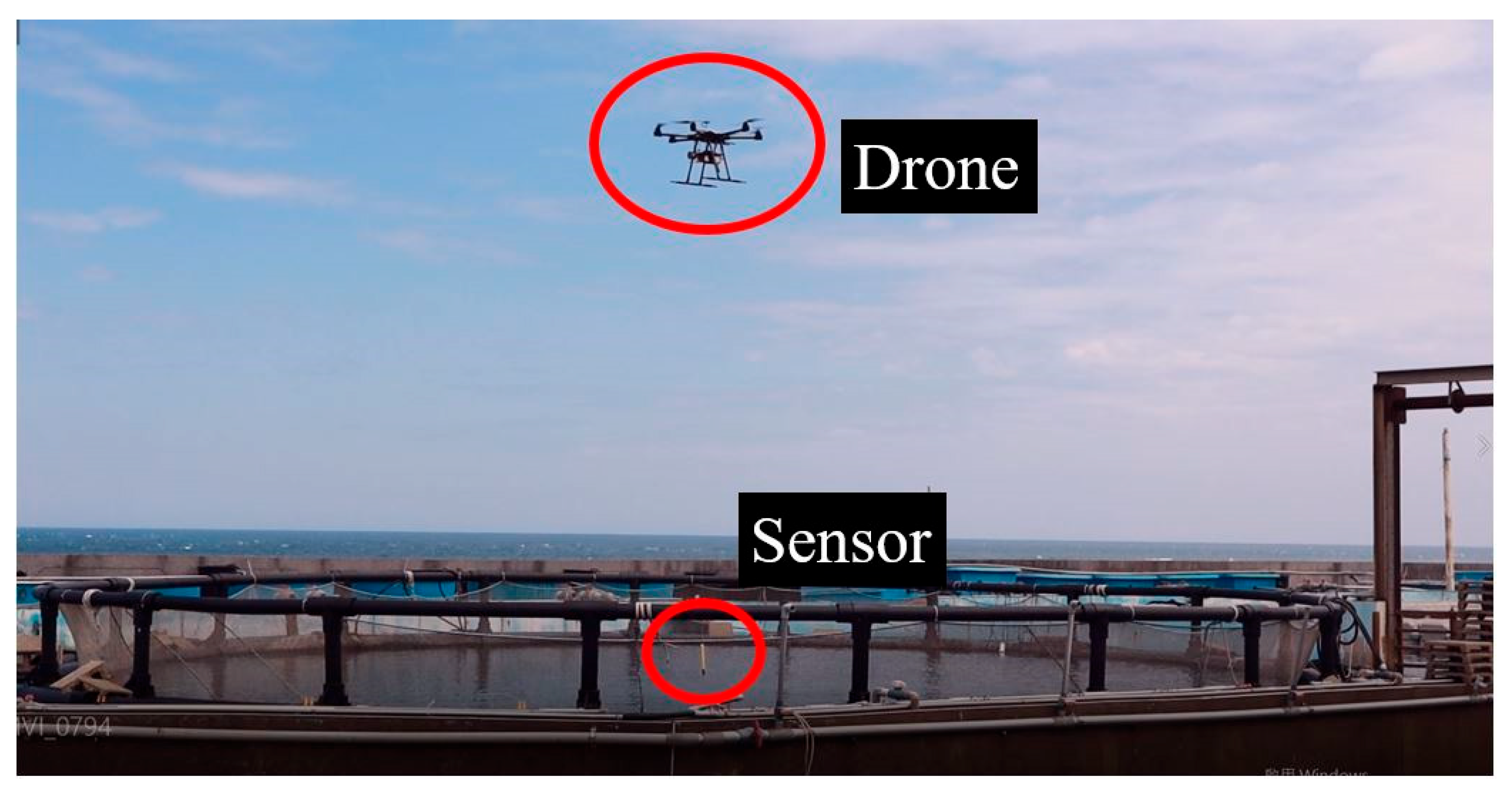
This study was mainly divided into two parts. The first part used an aerial camera, gimbal, and onboard processor to control the UAV approaching the net cage. A physical sensor was used to measure the water quality. A servo motor and sensor were used to collect cage water quality information. The second part consisted in establishing a cage data set and modifying the YOLO model so that the model could be applied to detect the cages. This study proposes a control scheme to solve cumbersome problems such as environmental data collection and net cage detection in aquaculture by using UAVs. We integrate assembled UAVs with peripherals such as onboard processors (Jetson TX2), cameras, servo motors, and sensors to enhance drone autonomy in aquaculture water quality measurement. Compared to commercial drones, we can adjust types of equipment and parameters according to requirements. The UAV uses an onboard camera to recognize the specified target and fine-tune its position to reach the destination more accurately. Different errors exist according to the quality of GPS. The general error of GPS is between 1 and 3 m. This study aims to use image assistance to correct the error. We use Pixhawk as the flight control board to control the flight. It is a platform with cruise functions and basic sensors. The Jetson TX2 is used as an onboard computer to control the Pixhawk, and image recognition is used to fix GPS errors and adjust the UAV position. In the neural network model adjustment, because the Jetson TX2 does not possess the computing power of a desktop computer, the image processing model selection is based on less computation and high accuracy criterion. The contributions of this study are listed as follows. (1) Modify the YOLO network to fit the net cage aquaculture task’s time requirement and reduce recognition errors. (2) Use the UAV’s onboard camera to recognize the specified cage and fine-tune the UAV position to reach the destination more accurately. (3) The UAV’s onboard physical sensors are used to measure water quality and obtain accurate values in aquaculture environment monitoring. (4) All operations are unmanned and automatic, saving detection and labor costs.

2. System Description

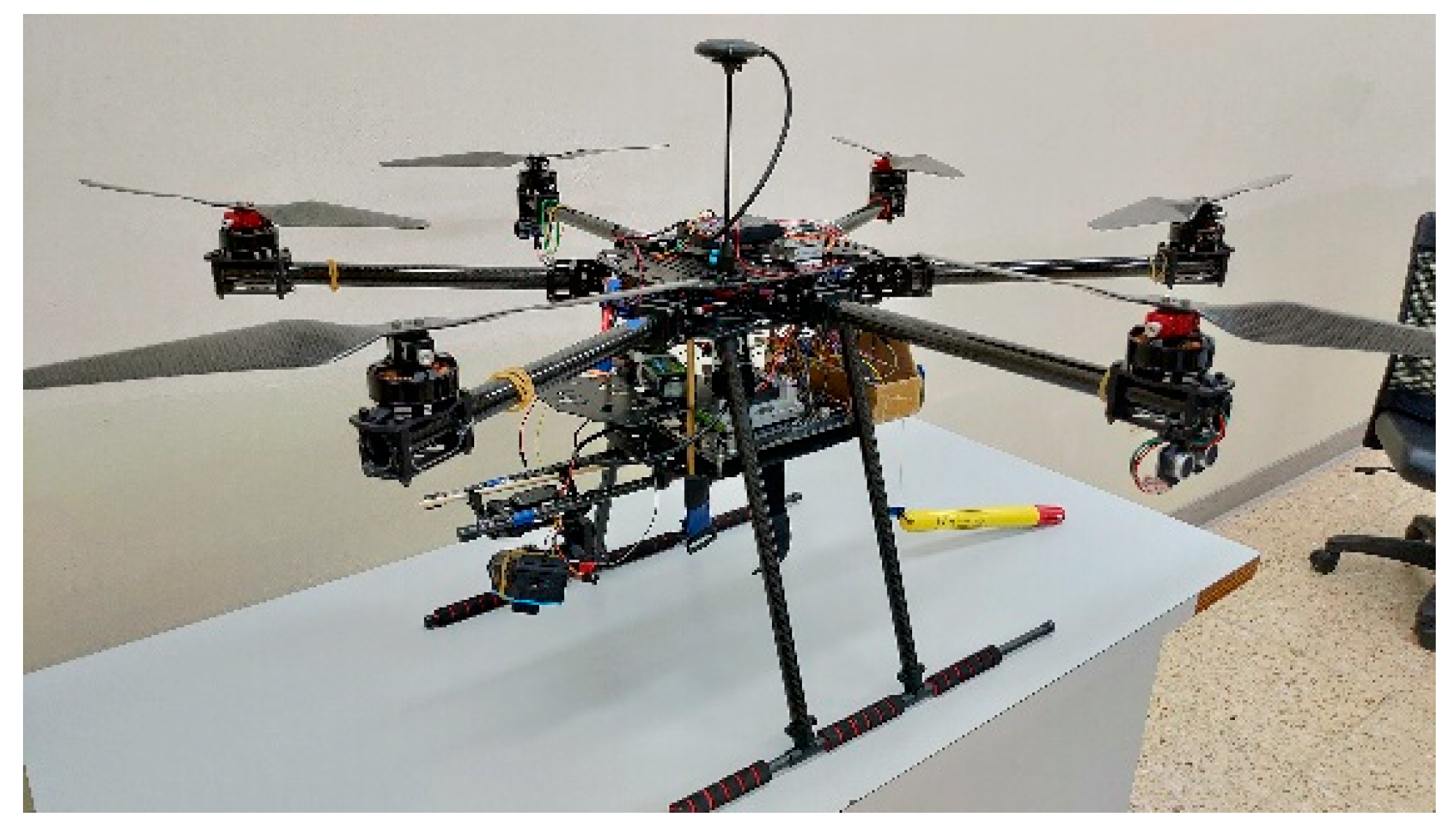
A hexacopter was assembled in this study, as shown in Figure 1. The system comprises a camera, onboard processor Jetson TX2, Pixhawk flight control board, GPS, water quality detector, and servo motor.

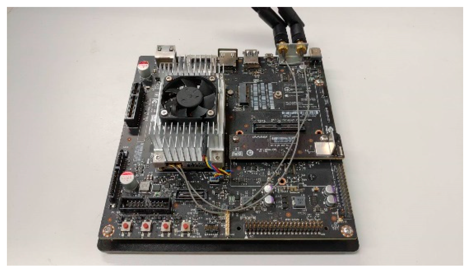
The Jetson TX2, produced by NVIDIA (Santa Clara, CA, USA), is a computing platform shown in Figure 2. It was designed specifically for machine learning computing [19]. The graphics processing unit (GPU) on the Jetson TX2 contains NVIDIA Pascal 256 CUDA GPU cores and a heterogeneous multi-processing (HMP) Dual Denver 2/2MB L2 and Quad ARM A57/2 MB L2 central processing unit (CPU). It is an excellent tool for deep learning models that can be trained and process new data faster than other computing platforms, such as Raspberry Pi and Arduino. Because of its lower weight and dissipated power, the Jetson TX2 is suitable for the drone. 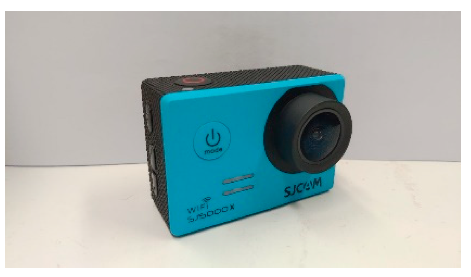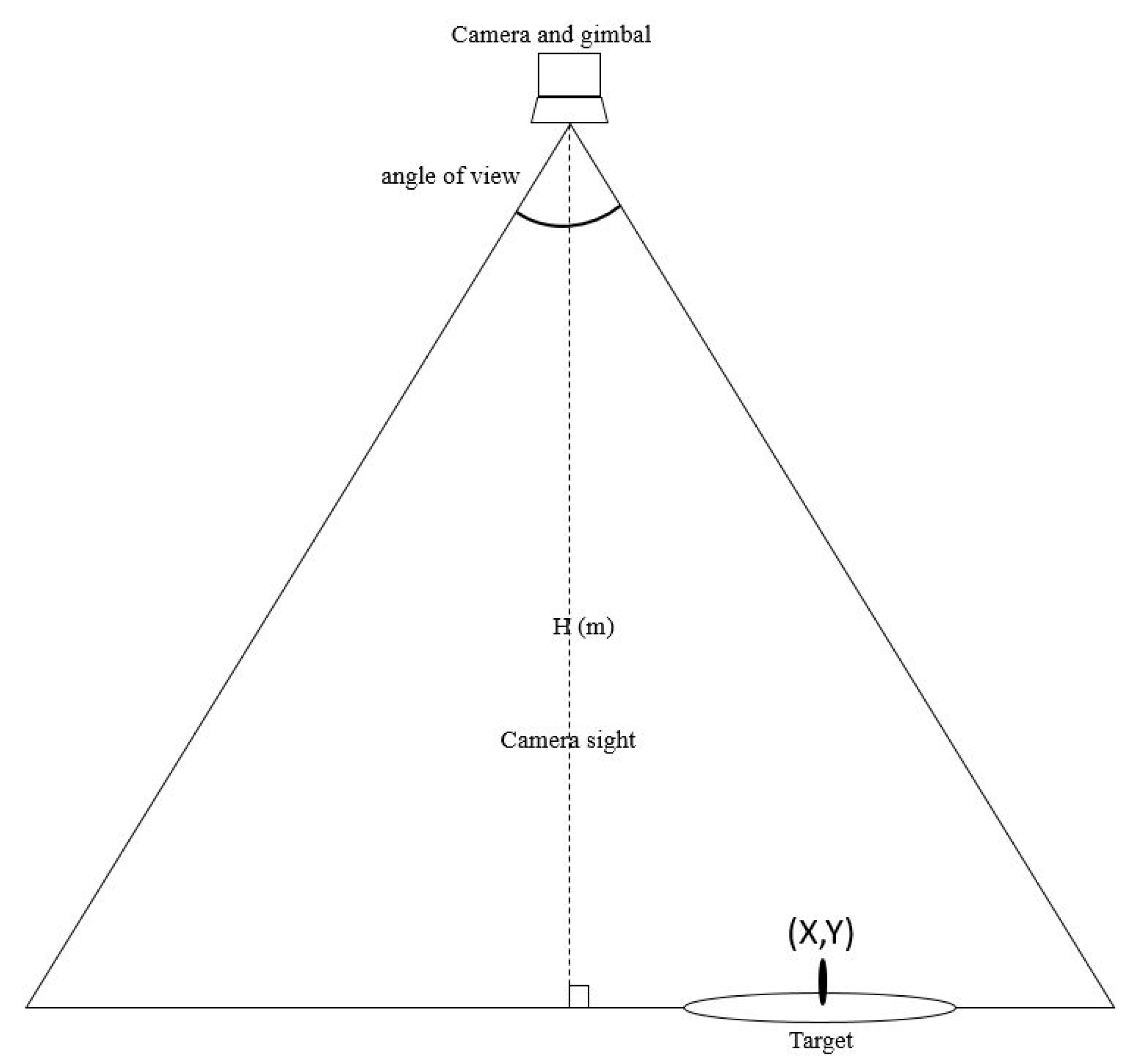Its operating system is Linux, which can run the Robot Operating System (ROS) [20]. Our study uses the SJCAM (Shenzhen, China) SJ5000X 1080P full-HD webcam, as shown in Figure 3. Its up-and-down viewing angle is 80 degrees, and its left and right viewing angles are 112 degrees. The camera streaming video pixel value is 12.4 million.

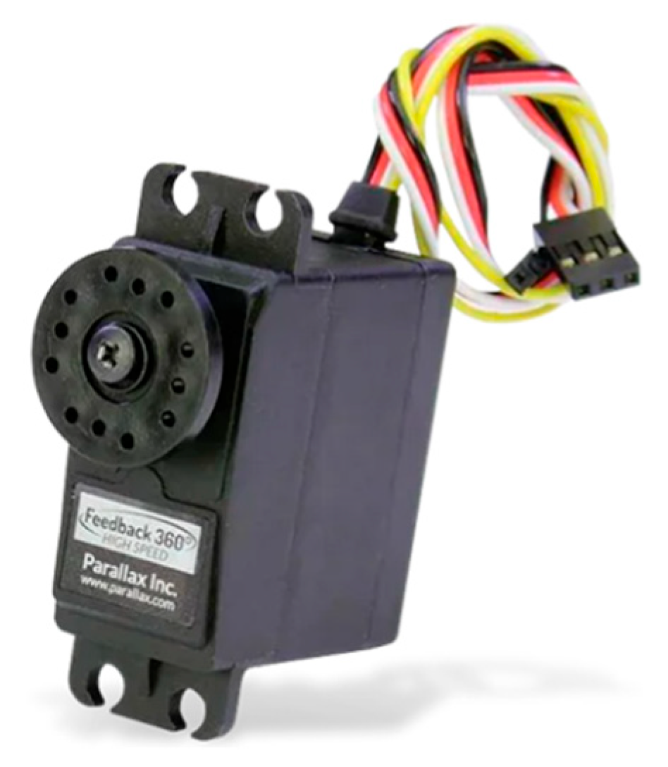
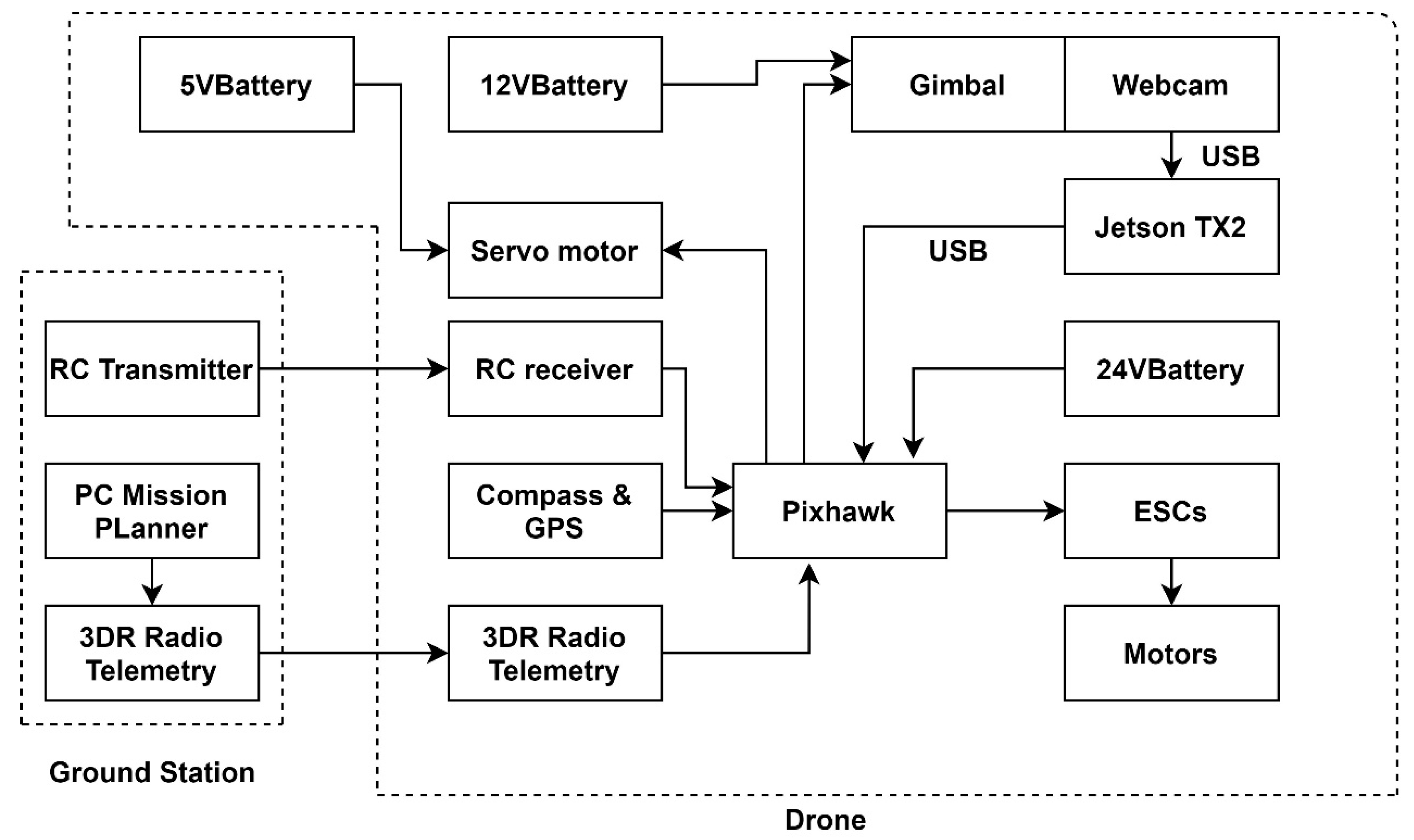
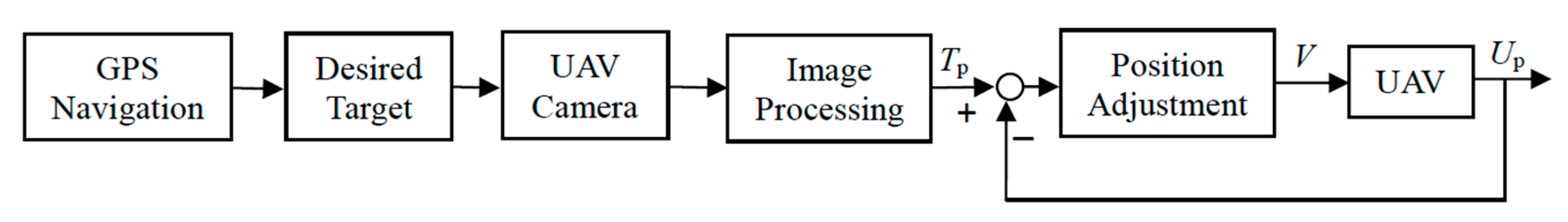
The primary purpose of this study is to collect various parameters of the cage environment (water temperature, water quality). We use a 360-degree servo motor to drop the sensor to measure water information. A faster motor is used. As shown in Figure 4, the 360° high-speed parallax feedback servo motor [21] has relatively low torque but high speed, and the working voltage is 5–8 V. We can use the Pixhawk flight control board to output PWM signals to control the motor. The weight of the motor is 45 g. At a voltage of 5 volts, a rotation speed of 100 per minute can lift heavy objects weighing up to 2 kg. The signal flow diagram of the overall drone hardware is shown in Figure 5.

3. Target Recognition

3.1. Network Structure

The architecture of YOLOv3 can usually be divided into a feature extraction layer and an output layer. The feature extraction layer is darknet-53, and the input image will first be converted to the architecture to use convolution for feature extraction. In the network, residual layer connections are designed between layers. The routing layer performs feature fusion, and the up-sample amplifies the features by a factor of 2. Finally, three YOLO layers are used as the output layer for detection. In the output part, if $416\times 416$ grid cells are used as input, the output has a certain characteristic size: $52\times 52$, $26\times 26$ and $13\times 13$, respectively. This feature size can detect small, medium, and big objects [22].

What is special is that in the entire YOLOv3 architecture, there is no pooling layer and a fully connected layer. The down-sampling part is done with convolutional layers. The anchor box replaces the part of the fully connected layer. The anchor box is a priori knowledge, the value generated during the training phase, and it uses the a priori box to predict the bounding box. The filter method will be adjusted during training to update the feature map. In the test phase, the bounding box of the target object can be generated by the length and width of the anchor box and the value predicted by the network. YOLO3 sets three types of anchors for each feature pyramid network (FPN) prediction feature map ($13\times 13$, $26\times 26$, $52\times 52$) box. Anchor boxes of nine sizes are clustered. For example, the nine anchor boxes in the COCO dataset are $(10\times 13)$, $(16\times 30)$, $(33\times 23)$, $(30\times 61)$, $(62\times 45)$, $(59\times 119)$, $(116\times 90)$, $(156\times 198)$, and $(373\times 326)$. The value of the anchor box is not the coordinate position, but the size of the anchor box (pixel value), which represents the length and width.

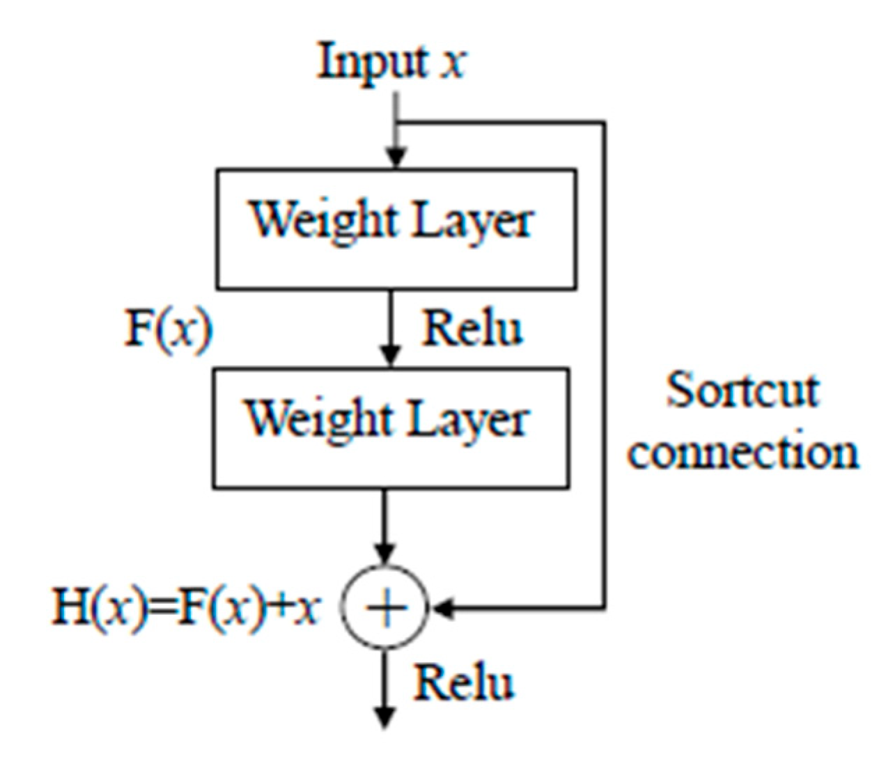
YOLOv3 primarily uses the residual network [23] to reduce the error rate of deeper neural networks. Traditional deep learning will face the problem of the disappearance of the backpropagation gradient when the network is more extensive than 100 layers. When the number of layers increases, the training and testing error rate will rise instead. In addition, shortcut connections are used for cross-layer connections, as shown in Figure 6. The input x is passed to the output as the initial result, and the output result is $\mathrm{H}\left(x\right)=\mathrm{F}\left(x\right)+x$. When $\mathrm{F}\left(x\right)=0$, then $\mathrm{H}\left(x\right)=x$. It can be understood that the learning objective has changed instead of learning a complete output, but for the difference between the learning objective values H(x) and x, the equation is $\mathrm{H}\left(x\right)=\mathrm{F}\left(x\right)+x$. Therefore, the following training goal is to approximate the residual result to 0 so that as the network deepens, the accuracy rate will also increase.

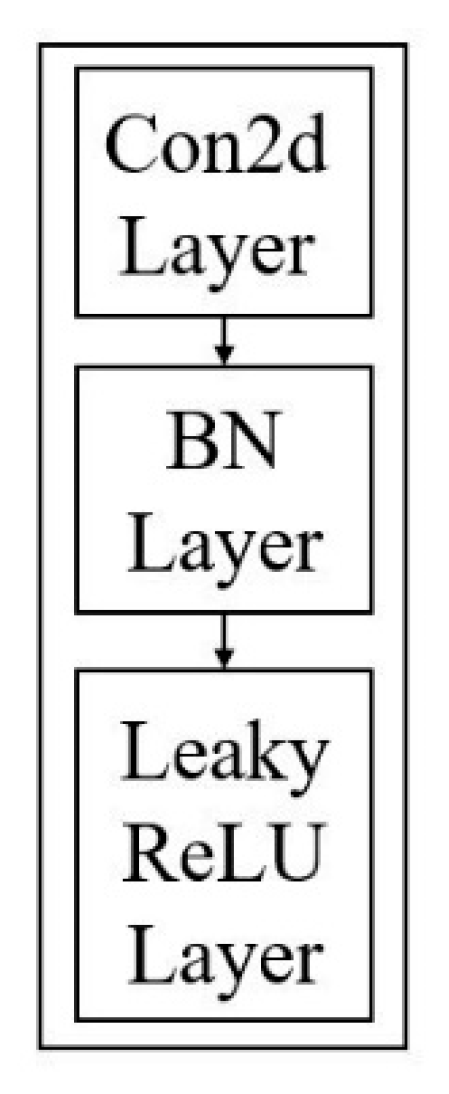
Figure 7 demonstrates the composition of the convolutional layer. It will be conv2D for 2-dimensional convolution, then normalized by the batch normalization layer [24], and output by the activation function. The purpose of batch normalization is to normalize training and reduce model overfitting. Because the distribution of training and test data is different, the effect of the network’s generalization ability is inferior. In addition, every batch training data distribution is different, so the network has to learn another distribution at each iteration, which will reduce the training speed. Batch normalization is the layer that prevents this result from increasing.

In the input part, the input size is $416\times 416$. If the size of the original image is not this, it will be scaled to $416\times 416$ according to the height-to-width ratio. The scaling equation is (1): w and h are the width and height of the original image, img_w and img_h represent the width and height of the input of the member image, input_w means the width of the converted image, and input_h represents the height of the converted image. This conversion formula can adjust the long side of the new image to the required input size of 416, while the short side is scaled without distortion. Regardless of training or testing, it is necessary to operate the original image.

$$\begin{gathered} {input}_w=im{g}_w\times (\mathrm{m}\mathrm{i}\mathrm{n}(w/im{g}_w,h/im{g}_h) \\ {input}_h=im{g}_h\times (\mathrm{m}\mathrm{i}\mathrm{n}(w/im{g}_w,h/im{g}_h) \end{gathered}$$

(1)

3.2. Detection Process

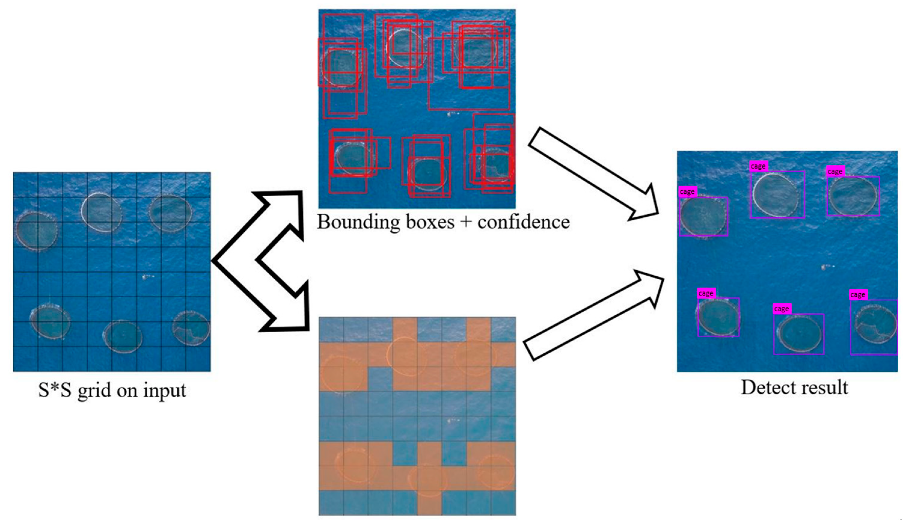
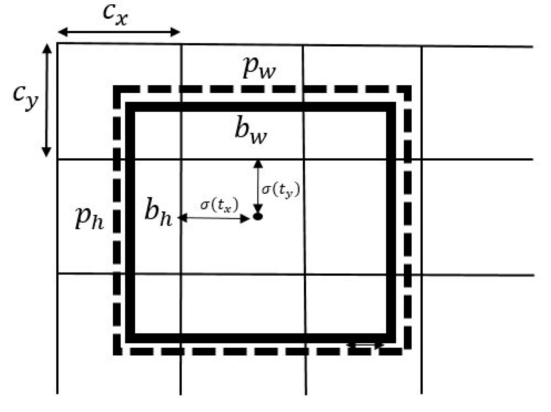
The original input image is divided into $\mathrm{S}\times \mathrm{S}$ grid cells [25], as shown in Figure 8. During training, each grid cell will predict N bounding boxes. Grid cells are used to detect different categories of targets. The network predicts the four coordinates of each bounding box, including the content contained in each of $t_x, t_y,t_w,\mathrm{a}\mathrm{n}\mathrm{d} t_h$, which are the offsets of the center of the bounding box prediction. $b_x$,$b_y$,${ b}_w$, and $b_h$ are the coordinates of the ground truth box. $\mathsf{\sigma }\left(t_x\right)$ and $\mathsf{\sigma }\left(t_y\right)$ are the distance from the center of the bounding box to its edge of the center cell, as shown in Figure 9. The detection process is shown in Figure 8. $C_x$ and $C_y$ are the coordinates of the upper-left corner of the cell, and each cell scale has a width and height of 1 in the feature map, so $C_x$ = $C_y$ = 1. In Figure 8, the center cell of this bounding box belongs to the grid cell in the second row and second column, and its upper-left corner coordinates are (1, 1). Among these, the dotted line represents the prediction box, and the solid line represents the ground truth. When training weights, the prediction box will match the ground truth more and more to achieve the training result.

The following equations can calculate the actual position and size of the bounding box:

$$\begin{gathered} b_{\mathrm{x}}=\sigma \left(t_x\right)+C_x \\ {b}_y=\sigma \left(t_y\right)+C_y \\ {b}_w=p_w{e}^{tw} \\ {b}_h=p_h{e}^{th} \end{gathered}$$

(2)

where ${ t}_x$, $t_y$, $t_w$, and $t_h$ are obtained by the following equations:

$$\begin{gathered} t_x=G_x-P_x \\ {t}_y=G_y-P_y \\ {t}_w=log(G_w/P_w) \\ {t}_h=log(G_h/P_h) \end{gathered}$$

(3)

$P_x$ and $P_y$ are the coordinates of the center point of the anchor box on the feature map. $P_w$ and $P_h$ are the width and height of the preset anchor box on the feature map. $G_x$, $G_y$, $G_w$, and $G_h$ are the ground truth center coordinates and the width and height coordinates of this feature map. C represents the probability that a bounding box contains an object. The confidence score is calculated as follows [26]:

$$\mathrm{C}=\mathrm{P}\mathrm{r}\mathrm{e}\left(\mathrm{o}\mathrm{b}\mathrm{j}\mathrm{e}\mathrm{c}\mathrm{t}\right)\times { \mathrm{I}\mathrm{O}\mathrm{U}}_{pred}^{truth}$$

(4)

Pre(object) indicates whether the bounding box may contain objects [27]. If there are targets in the bounding box, $\mathrm{P}\mathrm{r}\mathrm{e}\left(\mathrm{o}\mathrm{b}\mathrm{j}\mathrm{e}\mathrm{c}\mathrm{t}\right)=1$; if not, it is 0. IOU (intersection over union) is the ratio between the intersection area and union area of the predicted box ${box}_{pred}$ (predict) and the truth box ${box}_{truth}$ (ground truth), as shown in Equation (5).

$${\mathrm{I}\mathrm{O}\mathrm{U}}_{pred}^{truth}=area({box}_{pred}\cap {box}_{truth})/area({box}_{pred}\cup {box}_{truth})$$

(5)

During the test, the confidence score of a specific category in each bounding box is the probability that the category appears in the bounding box and the degree to which the prediction box matches the actual bounding box (ground truth). The confidence equation for each category and single bounding box is as follows:

$$\mathrm{C}\left(\mathrm{M}\right)=\mathrm{Pre}({class}_M\left|\mathrm{object}\right)\mathrm{Pre}\left(\mathrm{object}\right) {\mathrm{I}\mathrm{O}\mathrm{U}}_{pred}^{truth}=\mathrm{Pre}({class}_M){\mathrm{I}\mathrm{O}\mathrm{U}}_{pred}^{truth}$$

(6)

The network predicts three box proportions and then extracts features from those scales. It uses an architecture similar to the feature pyramid network (FPN) method to extract features of 3 scales. The prediction result of the network is a 3D tensor that is $\mathrm{S}\times \mathrm{S}\times (\mathrm{B}\times \left(5+\mathrm{C}\right))$. This study used three boxes to predict each scale, four anchor coordinates, one object score, and one category prediction. The tensor is $\mathrm{S}\times \mathrm{S}\times (3\times \left(1+4+1\right))$.

3.3. Model Evaluation

To improve the identification speed and accuracy, this study also improves network structure and compares the improved model with the original model. Finally, the ideal model is selected for the aquaculture mission so that the experiment can have the best results [28]. Many models can solve the object identification problem, but a type of evaluation effectiveness is needed. This study uses the following commonly used indicators for evaluation:

(1)

mAP (mean average precision)

(2)

FPS (frames per second)

(3)

BFLOPs (billion float operations)

A confusion matrix in machine learning is a result analysis table using evaluation algorithms or classifiers. Each column represents the predicted value, and each row represents the actual value [29]. The four elements of the confusion matrix (TP, TN, FP, FN) are shown in

Table 1. Confusion matrix.

Confusion Matrix		Ground Truth
		Positive	Negative
Predict	Positive	TP	FP
	Negative	FN	TN

[30]. TP (true positive) is a positive sample that correctly predicts success. For example, in an image classifier that predicts whether it is a target, if it is successful, label the picture of the target object in the prediction box, which is TP. TN (true negative) is the negative sample that correctly predicts success. FP (false positive) is the false prediction of a positive sample, which is actually a negative sample. FN (false negative) is a positive sample that cannot be predicted. When the predicted IOU exceeds the threshold (set to 0.5 in this experiment), it is considered a TP. If it is less than this threshold, it is an FP. As shown in Figure 10, blue is the ground truth, green is TP, red is FP, and pink is FN.

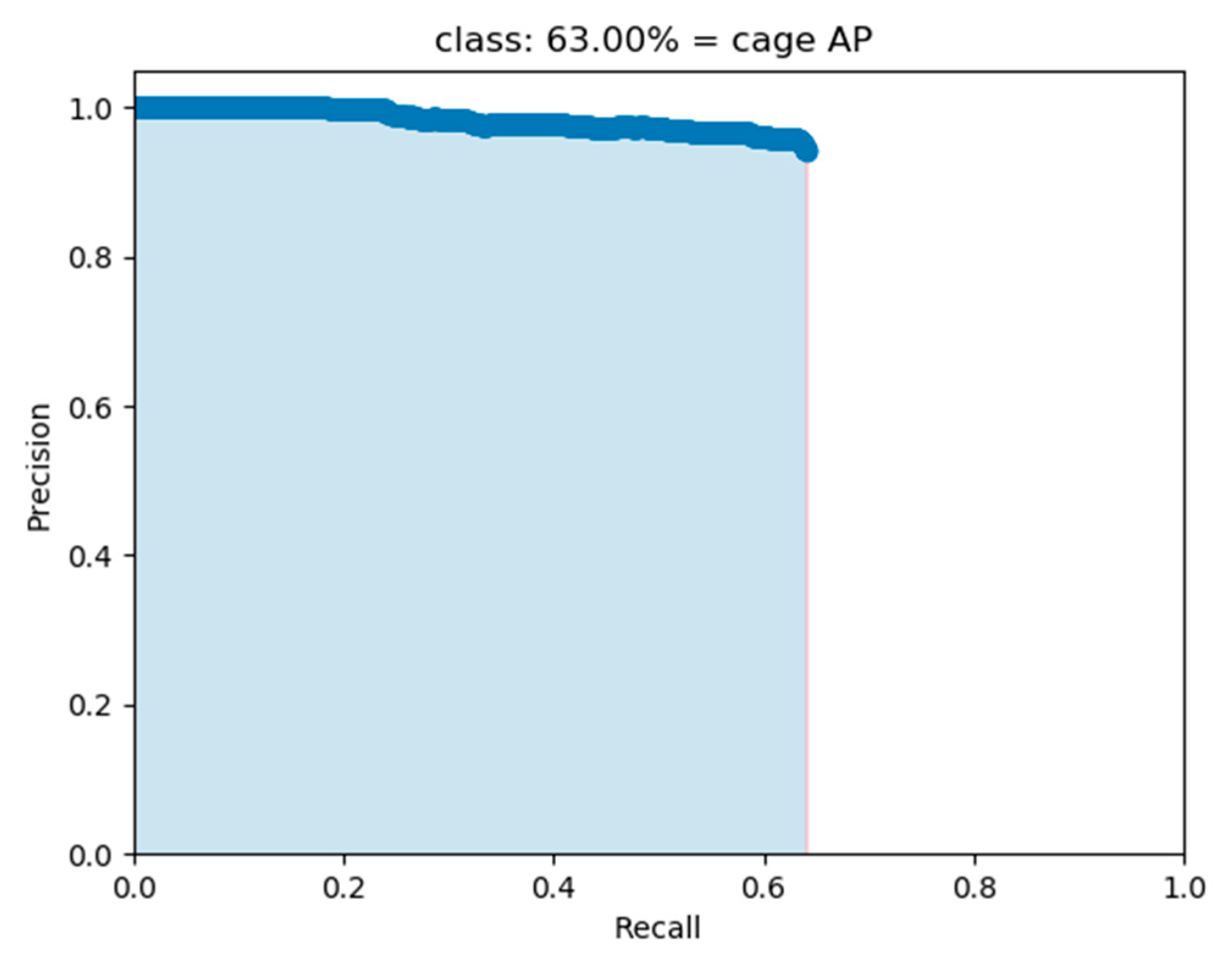
The concept of a confusion matrix is used to calculate precision and recall. The equations are given as follows:

$$\mathrm{Precision}=\mathrm{T}\mathrm{P}/(\mathrm{T}\mathrm{P}+\mathrm{F}\mathrm{P})$$

(7)

$$\mathrm{Recall}=\mathrm{T}\mathrm{P}/(\mathrm{T}\mathrm{P}+\mathrm{F}\mathrm{N})$$

(8)

The PR curve (precision–recall Curve) is shown in Figure 11, with recall as the X-axis and precision as the Y-axis. The maximum value of the X-axis and Y-axis are both 1. There is usually an inverse relationship between precision and recall rate. We can reduce one of their values as a cost to increase precision or recall rate. The area under the curve is AP, the equation is (9), and the larger the area, the better the result. The larger the area under the curve, the higher the precision and recall rate, and the easier it is for the model to detect the target. In this study’s experiment, because the target that needs to be detected is only one (cage), AP is also equal to mAP.

$$\mathrm{AP}=\mathrm{Average} \mathrm{Precision}={\sum }_{k=1}^{N}P\left(k\right)∆recall\left(k\right)$$

(9)

3.4. Improvement Model Comparison

The BFLOPs indicate how many billion floating-point operations are required for convolution operations; the full name is billion float operations. The complexity of the algorithm model can be expressed by adding up the BFLOPs consumed by operations such as multiple convolutions. The larger the value is, the greater the processor performance required by this algorithm model. FPS refers to frames per second. The video film is a continuous picture composed of pictures, and each image is in every frame of the film. A higher FPS has a better object identification effect when testing the model. On the contrary, with low FPS, the object identification effect decreases. In this study, considering the flying speed of the UAV, the FPS is controlled to not less than 3 to carry out the mission. During training, several parameters are fixed, as shown in

Table 2. Parameter settings.

Batch Size	64
Learning Rate	0.001
Subdivisions	16
Max Iteration	8000
Input Size	416 × 416

.

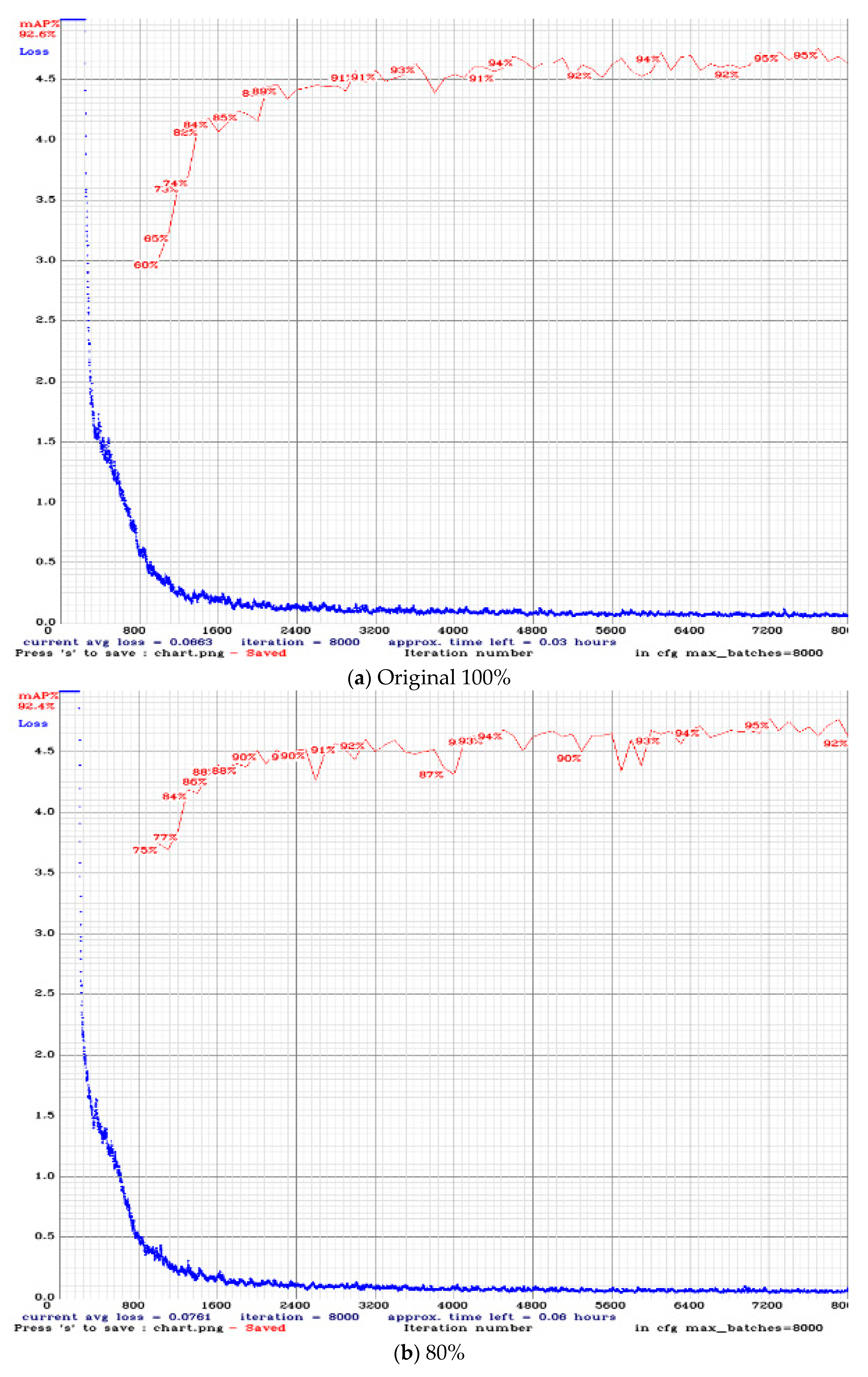
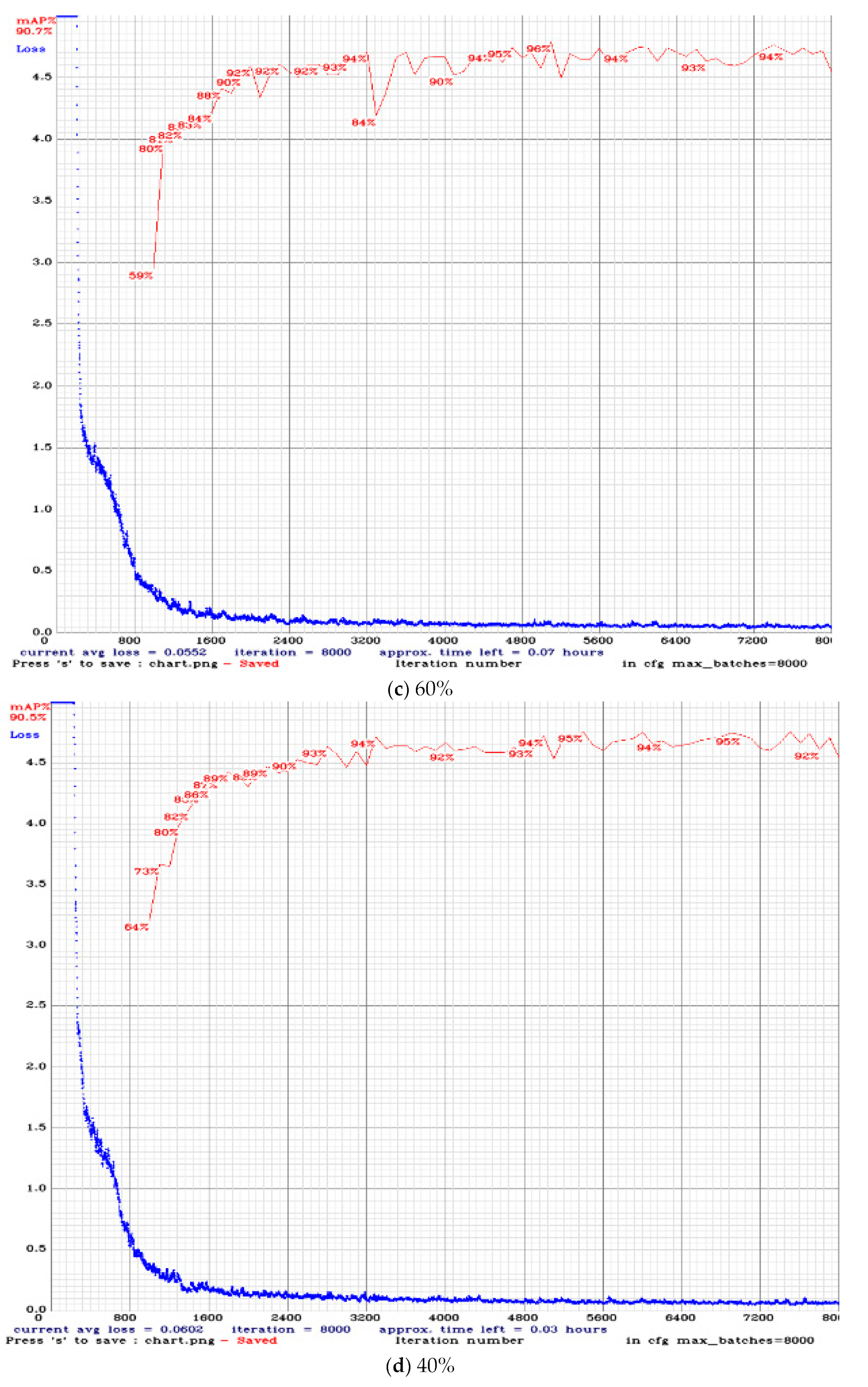
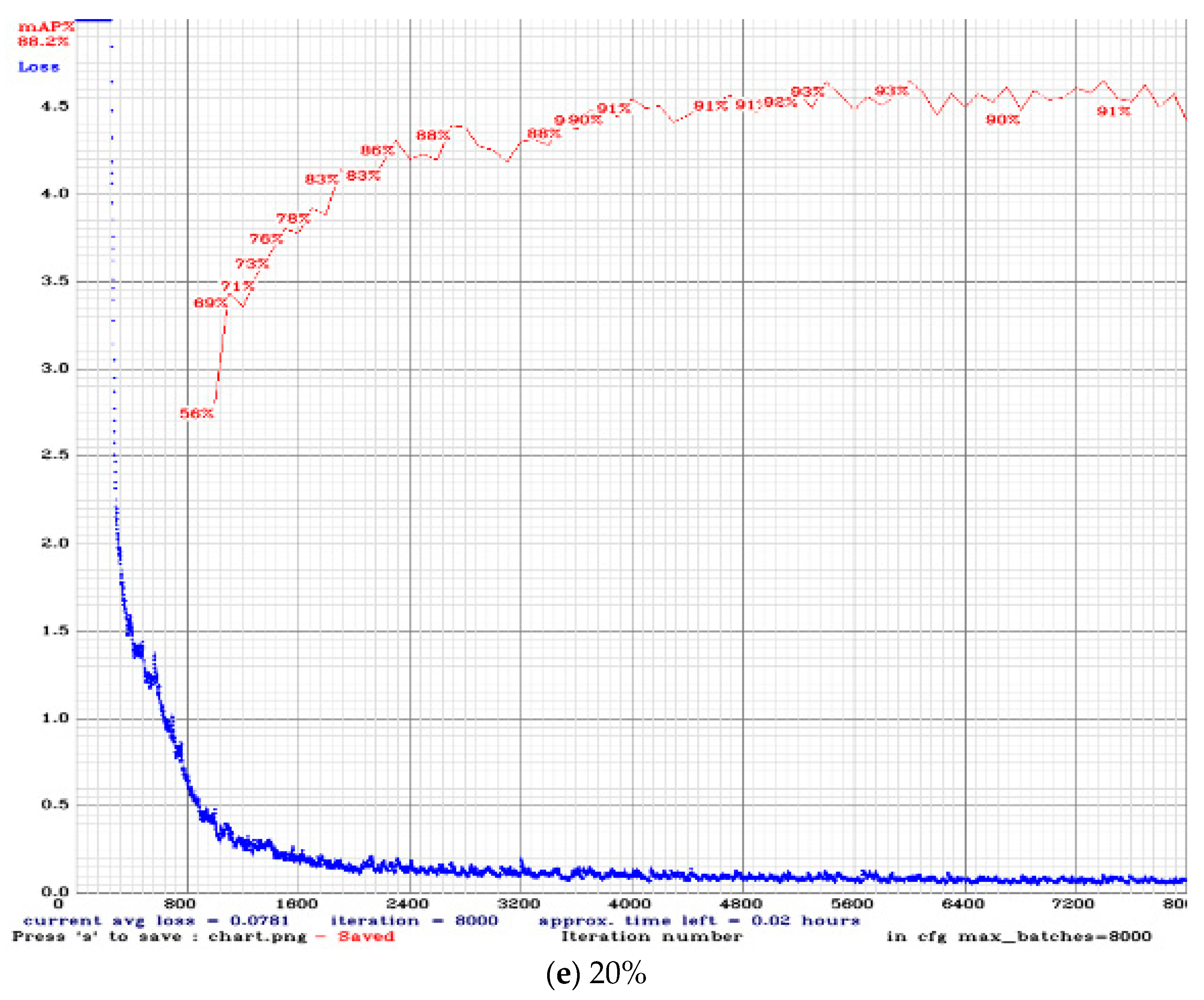
According to the relevant network structures, the model of YOLOv3 can be improved by reducing the number of filters in all convolutional layers. Take the image input of resolution $416\times 416$ as an example and compare it with the original network. The loss and mAP curves during training are shown in Figure 12a–e. Comparisons of different numbers of filters are shown in

Table 3. Comparisons of different numbers of filters.

Test Experimental Platform: Desktop Computer
Filters	Original 100%	90%	80%	70%	60%
FPS	98.2	107.6	119.5	139.2	148.1
BFLOPs	65.304	53.664	43.166	30.943	23.109
mAP	92.6	91.4	92.4	91.7	90.7
Test Experimental Platform: Jetson TX2
FPS	3.28	3.52	3.91	4.66	5.15
mAP	92.6	91.4	92.4	91.7	90.7
Test Experimental Platform: Desktop Computer
	50%	40%	30%	20%	10%
FPS	173.5	188.6	204.8	237.7	252.2
BFLOPs	16.415	10.864	6.454	3.456	1.953
mAP	90.3	90.5	89.9	88.2	84.7
Test Experimental Platform: Jetson TX2
FPS	6.51	7.32	8.29	9.89	10.31
mAP	90.3	90.5	89.9	88.2	84.7

.

The original network input is $416\times 416$. However, it may have different mAP and calculation amounts at various resolutions.

Table 4. Input size comparison.

Test Experimental Platform: Desktop Computer
Image size	$384\times 384$	$416\times 416$	$544\times 544$	$608\times 608$
mAP	91.3	92.6	93.1	93.5
FPS	107.6	98.2	86.5	79.2
BFLOPs	55.644	65.304	112.095	137.821
Test Experimental Platform: Jetson TX2
mAP	91.3	92.6	93.1	93.5
FPS	4.55	3.28	2.15	none

shows the comparison at various resolutions. In the adjustment of the input size, the side length is adjusted in multiples of 32 because the down-sample magnification used by the network is 32. The minimum image size used for training is $320\times 320$, and the maximum image size is $608\times 608$. This allows the network to adapt to different input scales [7]. When the input value is $608\times 608$, Jetson TX2 is unable to load the image due to too much calculation.

For filter improvements, as seen from Table 3, when using more filters, the lower the calculated value, the higher the FPS. However, mAP can still maintain about 90%. In other studies [30,31], when the number of filters continues to decrease, the mAP will also decrease correspondingly in theory. However, in this experiment, the mAP is not reduced significantly. The possible reason is that the identified target has a fixed outline and still has apparent characteristics under different angles and light. Therefore, when the target is relatively easy to identify, a less structured model can be used for identification, and the required filter can also be reduced. In different input resolutions, when the input size is larger, mAP also increases, but the increment is small, and the BFLOPs increase significantly. However, because the current calculation of Jetson TX2 is not enough to use the $608\times 608$ input, the input size of the model we used will be lower than this input value. One can choose the appropriate model according to the flight environment and mission when conducting a flight mission. In this study, the target to be identified is relatively simple, and the appearance change is not complicated. In addition, because the Jetson TX2 is used for calculations, it can perform tasks with a high FPS and a certain degree of accuracy.

3.5. Target Recognition

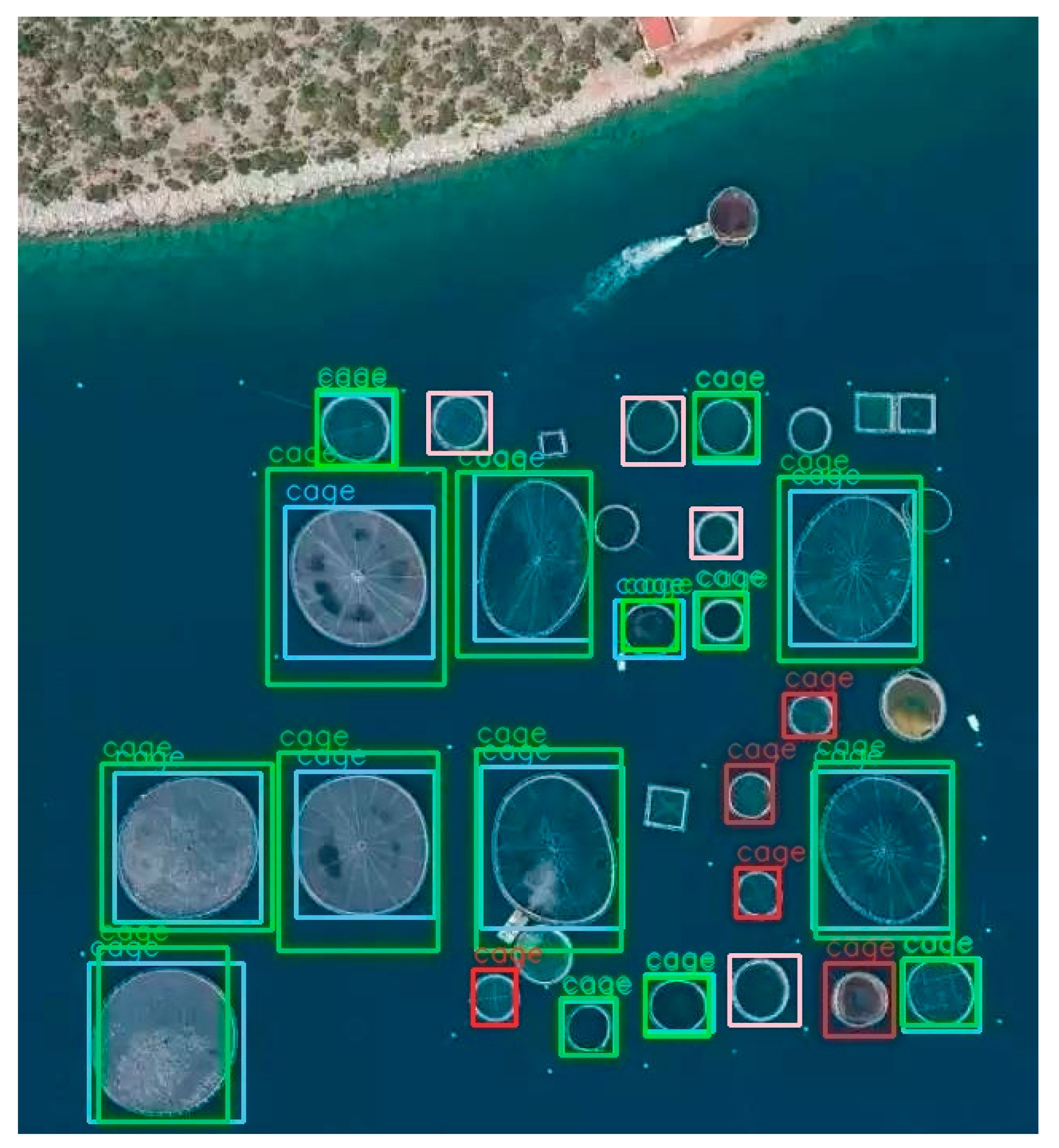
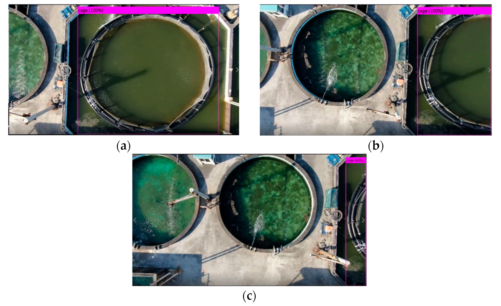
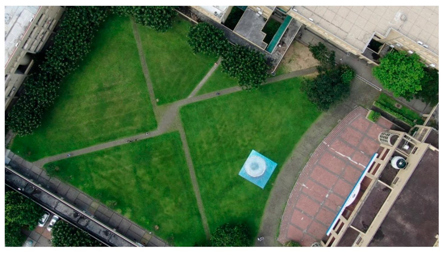
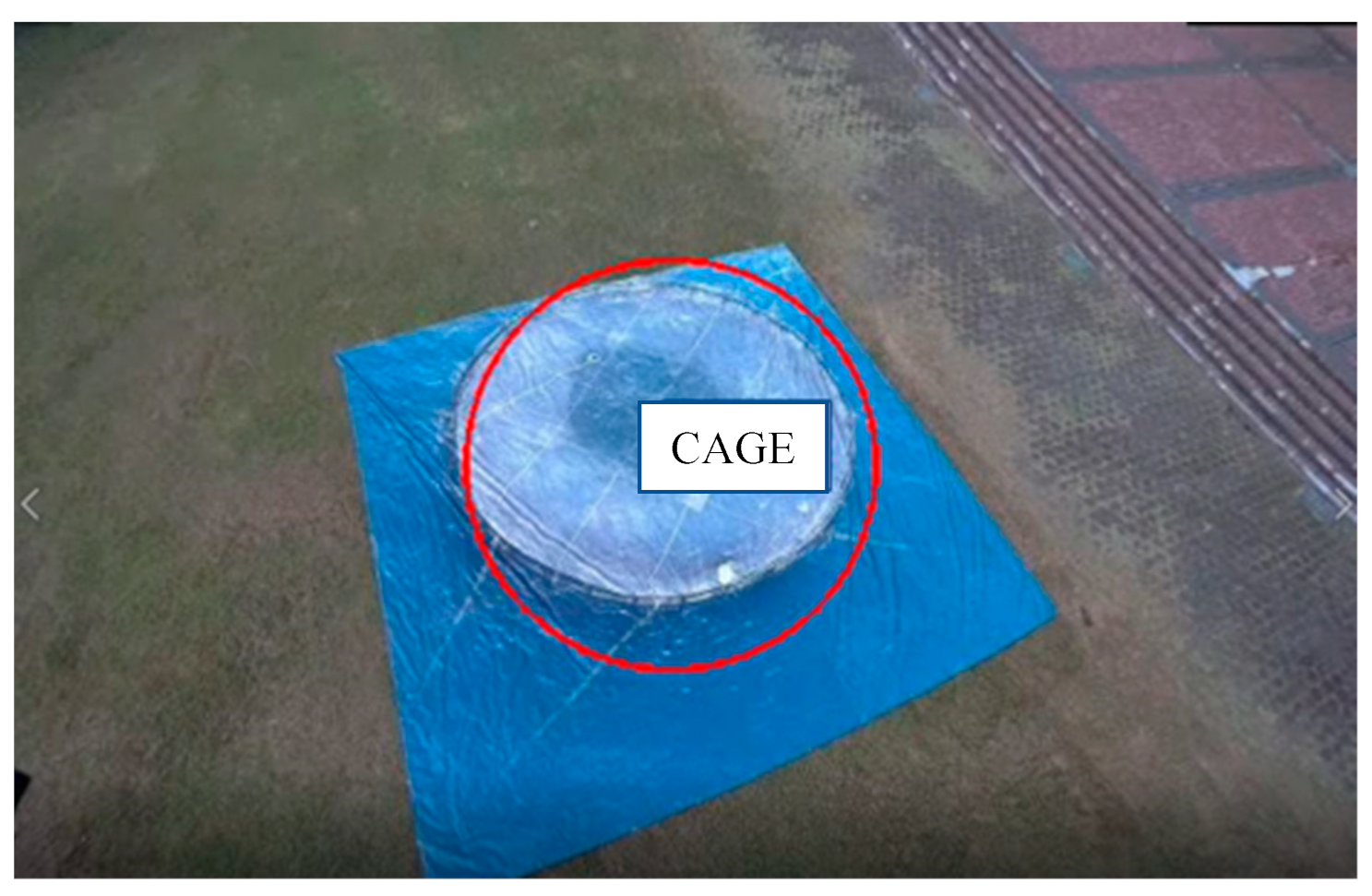
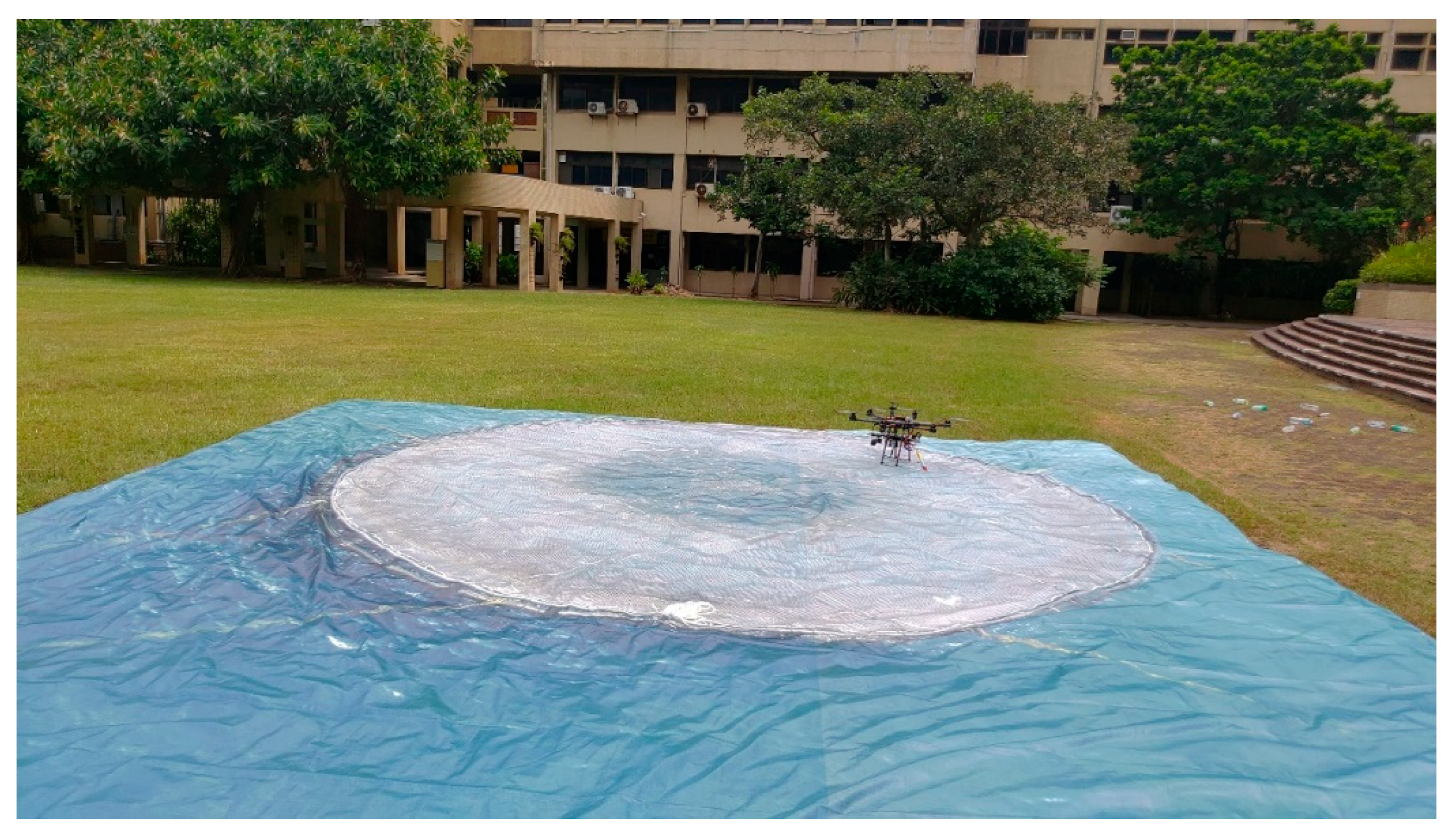
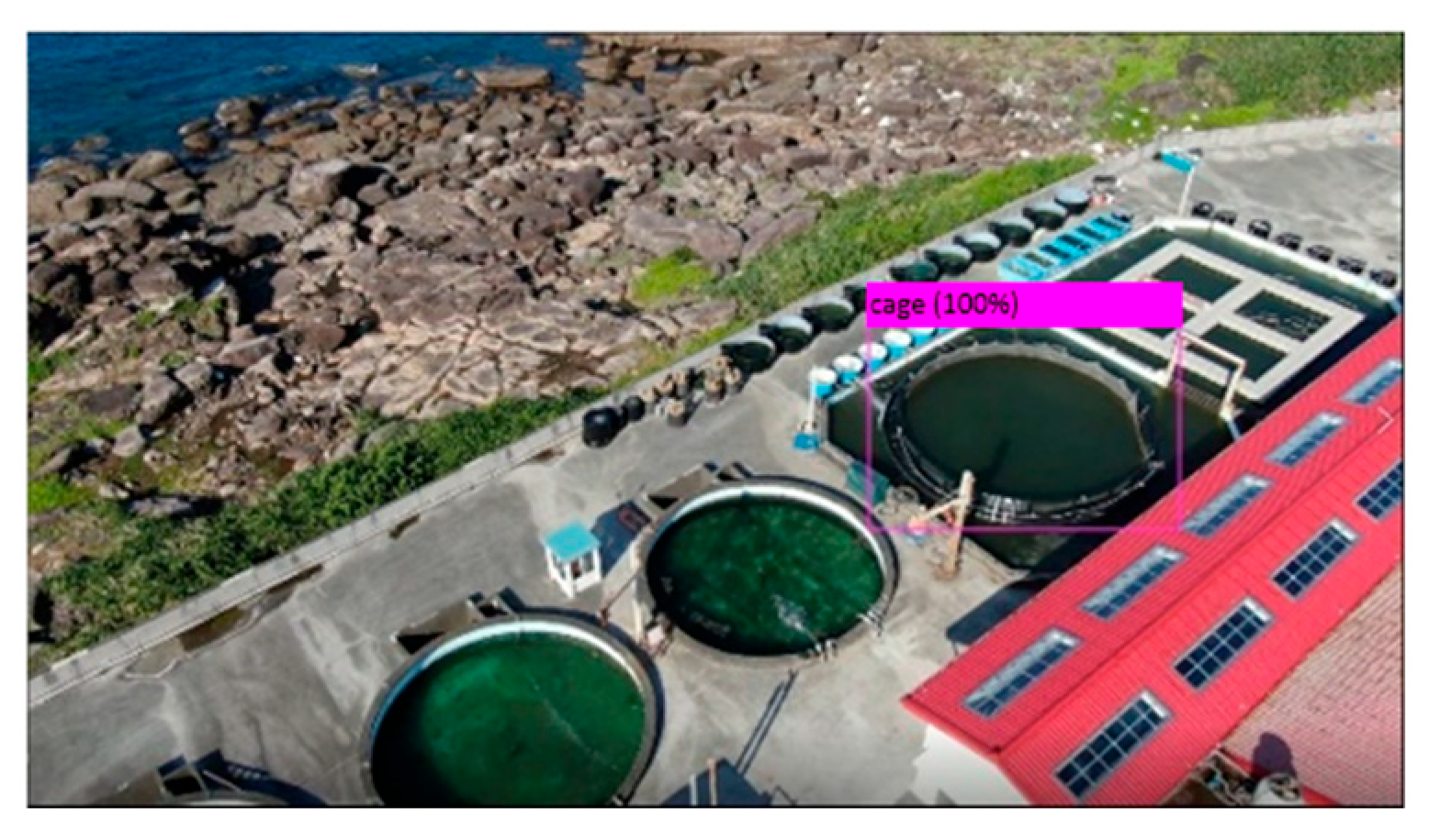
In this study, we collect authentic net cage images from different angles as data for training and testing to increase the accuracy of object recognition. The vertical top view of the ground target is shown in Figure 13. The UAV’s flying height is 10 m, and the diameter of the net cage is 10 m. The effect of the net cage coverage area on the confidence score can be observed. In a wholly uncovered situation, the confidence score is 100%. 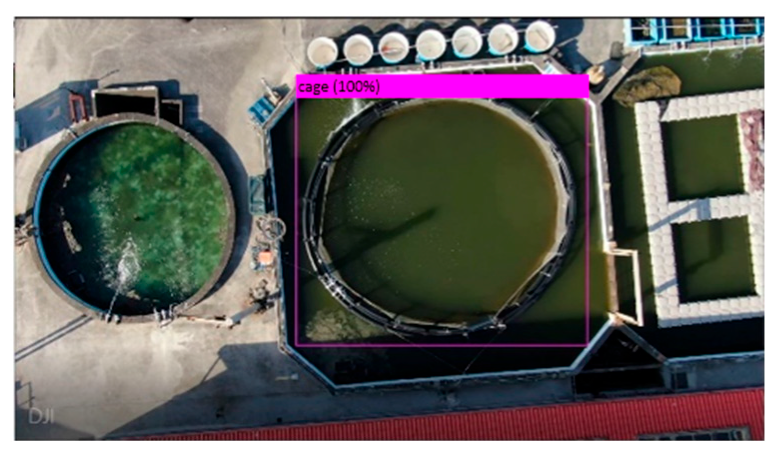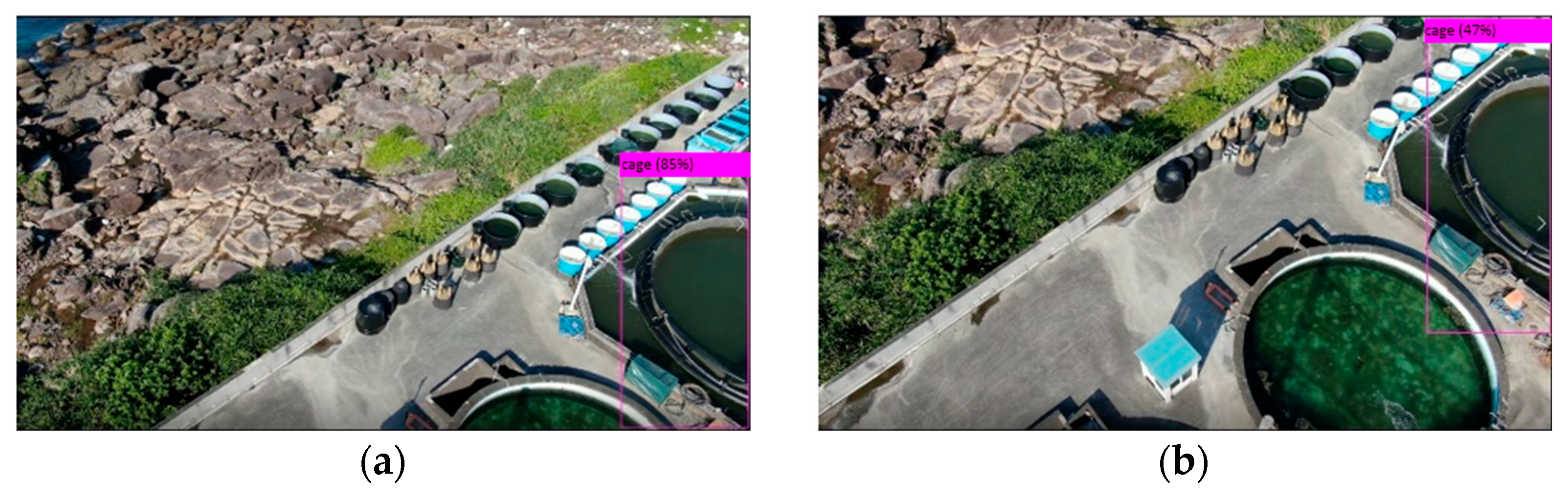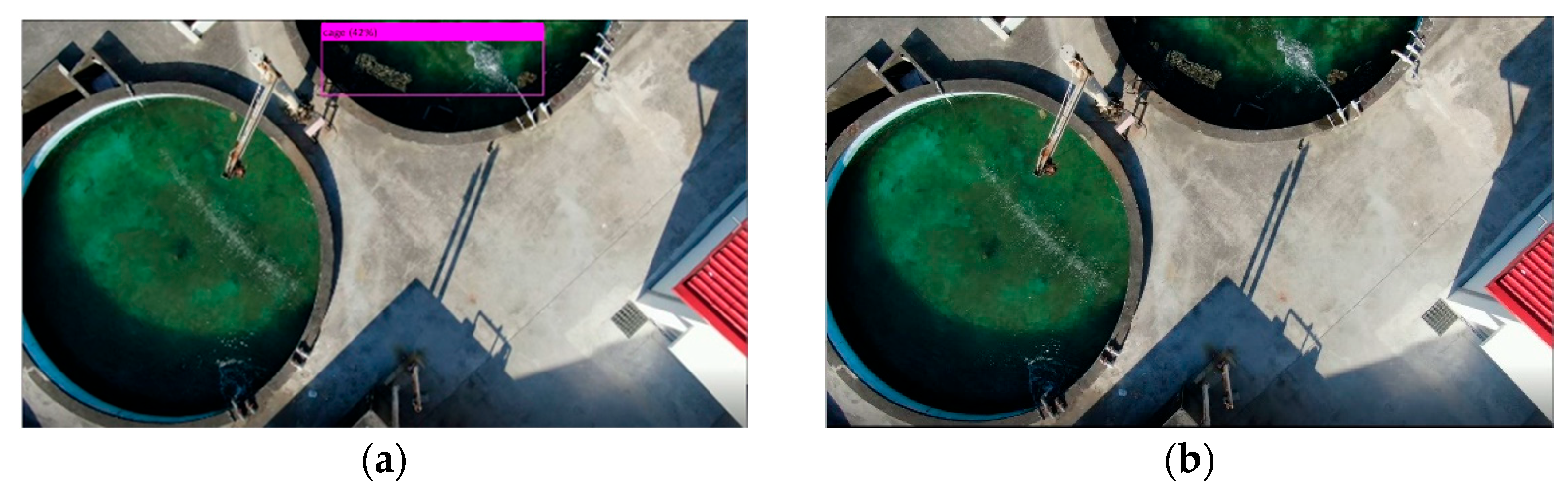Figure 14 shows a similarly shaped object (pool) on the left side. The target cage can still be recognized with a 100% confidence score. When covering (blocking) 50% of the target area, the confidence score is also 100%, but when blocking about 90% of the area, the confidence score is only 40%. 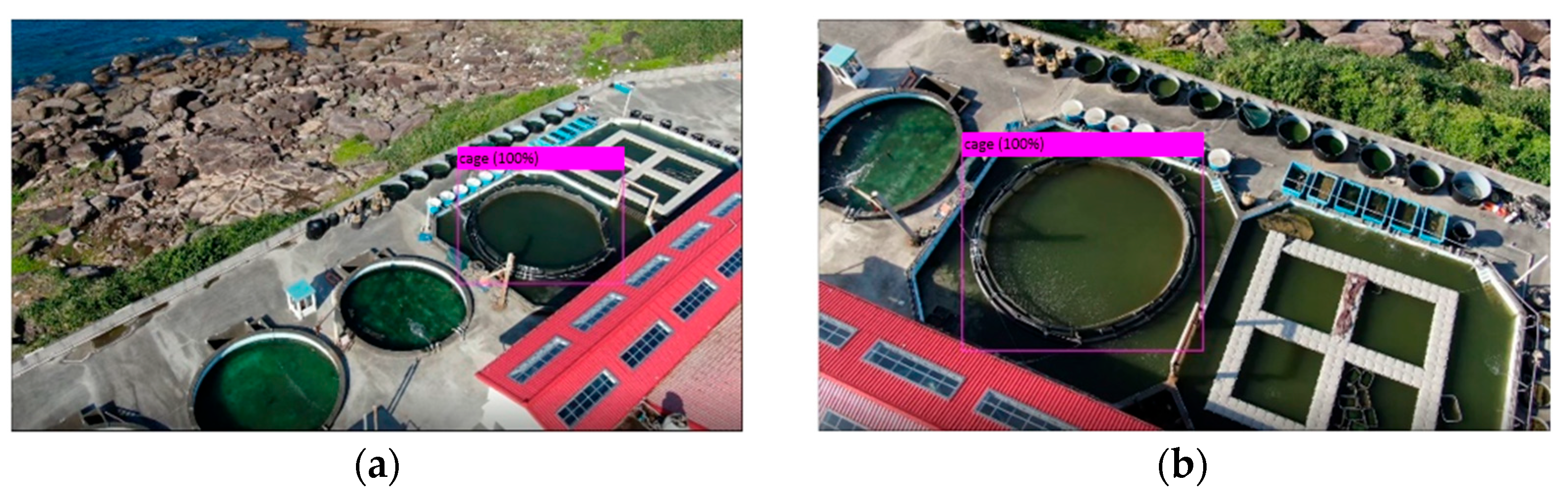In the part of the side-view net cage, when the model is identified in different coverage areas, as shown in Figure 15, the confidence scores are 85% and 47%, respectively. The confidence score is also approximately proportional to the coverage area. Their confidence scores are all 100% when identified from different angles, as shown in Figure 16. The identification effects of the above experiments can meet the flight mission requirements in this study. The confidence score can also be high when the coverage area is large. In addition, although the characteristics of the target and the pool on the left side are very similar, there will be no confusion, as shown in Figure 14.

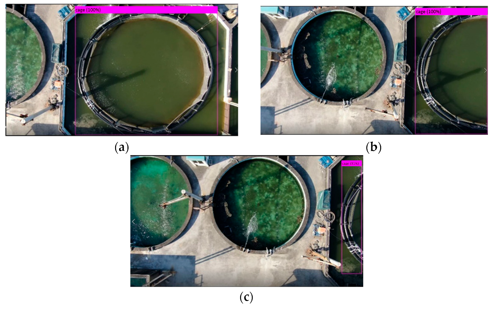
In the experiment for reducing the filter model, the net cage can be identified in the part where the number of filters is reduced to 90%, as shown in Figure 17 and Figure 18a,b. However, when the coverage rate is 90%, the confidence score of the net cage drops to 31%, which is lower than the confidence score of the original model, as shown in Figure 18c. When identifying from other viewing angles, the target may be recognized incorrectly (FP), as shown in Figure 19a,b. Figure 19a shows that the model of 10% filters is used. It can be seen that the pool will be recognized as a cage, which is an error recognition. Figure 19b is the result of recognition using the original model. On the same screen, there is no recognition error.

The identification effect will also be better with an increase in the number of data points, but after a certain amount is reached, the mAP value will no longer increase significantly. After repeated experiments, when training the net cage, if it is taken on the vertical top view, only about 500 images are sufficient as data. If it is a side view, one needs to collect net cages with different angles, and a number of data points between 1500 and 2500 can achieve the best recognition effect. The more diverse the image angle and the lightness used, the better the training effect will be.

4. Control Scheme

4.1. Control Sequence

This study uses an aerial camera to capture the cage position and adapt the UAV position. First, the weight of the neural network with the cage image is trained. Then, the weight is used in the network. Use Jetson TX2 to execute the network to identify the target cage. Jetson TX2 can control the UAV through the Pixhawk board. The flowchart of the control sequence is shown in Figure 20. The UAV is planned to cruise several net cages through the GPS. The drone will first fly to the target region and then let the drone start to rotate in place and rotate at most one circle. When the drone recognizes the target, it will stop spinning, and the processor will translate the drone’s left and right movements to render the target located at the centerline position of the camera screen. After that, the drone will move forward and change the pitch angle of the gimbal to keep the picture consistent. When the angle of the gimbal is lower than the set value, the drone will adjust the position of the front, back, left, and right, and finally change the position of the drone to directly above the target; the drone will then use the servo motor to drop the sensor and perform the work we set up in advance. After that, the drone will fly to the next destination until the mission is completed. All steps are automatically controlled by the Jetson TX2 on the UAV.

4.2. Gimbal Angle Adjustment and UAV Movement

Rotate the UAV and adjust the target to be shown on the center line, as shown in Figure 21. The input pixel of the camera screen is $640\times 480$. After that, the drone will adjust the pitch angle of the gimbal and allow it to fly forward. The two actions are synchronized. The angle of the gimbal must change as the drone moves. The coordinate diagram of the camera screen is shown in Figure 21. The center coordinates of the target object’s bounding box are (X, Y). When the Y coordinate is greater than 240, it means that the target object is located in the upper half of the camera screen. In Figure 22, A is the current angle (degree) of the gimbal, CA is half of the camera’s angle (degree), H is the flying altitude of the drone (m), and B1 is the angle (degree) of the vertical ground line between the target and the drone. After calculating through Equation (10), distance (m) is the straight-line distance between the drone and the target. When the Y coordinate is less than 240, the adjustment method is as in Equation (13), which means that the target is located in the lower half of the camera screen.

If the target is in the upper half of the screen, the complete calculation steps are as follows:

(1)

Use Equation (10) to calculate the distance.

(2)

Equation (11) calculates the angle between the target and the drone perpendicularly to the ground, which is set to B1, as shown in Figure 22.

(3)

Bring the distance into the judgment interval of Table 5 to get the drone’s moving distance (m) in a second, as shown in Figure 22.

(4)

Use Equation (12) to calculate the angle of the gimbal rotation, followed by the drone’s vertical ground line, as shown in Figure 23.

(5)

Calculate the rotation angle of the gimbal, which is B1–B2.

(6)

Move the drone and rotate the angle of the gimbal, as shown in Figure 24.

(7)

Repeat steps 1 to 6 until the gimbal angle is less than D. E is the length or diameter of the target, as shown in Equation (16), and the schematic diagram is shown in Figure 25.

$$\mathrm{D}\mathrm{i}\mathrm{s}\mathrm{t}\mathrm{a}\mathrm{n}\mathrm{c}\mathrm{e}=\mathrm{H}\left(\mathrm{t}\mathrm{a}\mathrm{n}\right(\mathrm{A}\left)\right)+\left[\right(|\mathrm{Y}-240|/240\left)\right(\mathrm{t}\mathrm{a}\mathrm{n}(\mathrm{A}+\mathrm{C}\mathrm{A})-\mathrm{t}\mathrm{a}\mathrm{n}\left(\mathrm{A}\right)\left)\mathrm{H}\right]$$

(10)

$$\mathrm{B}1={\mathrm{t}\mathrm{a}\mathrm{n}}^{-1}(\mathrm{D}\mathrm{i}\mathrm{s}\mathrm{t}\mathrm{a}\mathrm{n}\mathrm{c}\mathrm{e}/\mathrm{H})$$

(11)

$$\mathrm{B}2={\mathrm{t}\mathrm{a}\mathrm{n}}^{-1}((\mathrm{the} \mathrm{d}\mathrm{i}\mathrm{s}\mathrm{t}\mathrm{a}\mathrm{n}\mathrm{c}\mathrm{e} \mathrm{done} \mathrm{moving})/\mathrm{H})$$

(12)

Figure 22. Schematic diagram of gimbal and camera. The upper right corner of each parameter indicates the degree symbol.

Figure 22. Schematic diagram of gimbal and camera. The upper right corner of each parameter indicates the degree symbol.

Figure 23. Gimbal rotation diagram.

Figure 23. Gimbal rotation diagram.

Figure 24. Drone movement diagram.

Figure 24. Drone movement diagram.

Figure 25. Gimbal minimum angle diagram.

Figure 25. Gimbal minimum angle diagram.

Table 5. Correspondence between the distance and flight speed.

Distance (m)	Drone Moving Distance (m/s)
0–10	1
10–20	1.5
20–30	2
30–40	2.5
40–50	3
>50	3

Table 5. Correspondence between the distance and flight speed.

Distance (m)	Drone Moving Distance (m/s)
0–10	1
10–20	1.5
20–30	2
30–40	2.5
40–50	3
>50	3

If the target is in the bottom half of the screen, the complete calculation steps are as follows:

(1)

Use Equation (13) to calculate the distance.

(2)

Equation (14) calculates the angle between the target and the drone perpendicularly to the ground, which is set to C1, as shown in Figure 26.

(3)

Bring the distance into the judgment interval of Table 5 to get the drone’s moving distance (m) in a second, as shown in Figure 26.

(4)

Use Equation (15) to calculate the angle of the gimbal rotation, followed by the drone’s vertical ground line, as shown in Figure 27.

(5)

Calculate the rotation angle of the gimbal, which is C1–C2.

(6)

Move the drone and rotate the angle of the gimbal, as shown in Figure 24.

(7)

Repeat steps 1 to 6 until the gimbal angle is less than D (degrees). E is the length (m) or diameter of the target, as shown in Equation (16), and the schematic diagram is shown in Figure 25.

Distance = H (tan(A)) − [((Y − 240)/240)(tan(A) − tan(A − CA))H]

(13)

$$\mathrm{C}1={\mathrm{t}\mathrm{a}\mathrm{n}}^{-1}(\mathrm{d}\mathrm{i}\mathrm{s}\mathrm{t}\mathrm{a}\mathrm{n}\mathrm{c}\mathrm{e}/\mathrm{H})$$

(14)

$$\mathrm{C}2={\mathrm{t}\mathrm{a}\mathrm{n}}^{-1}\left(\right(\mathrm{the} \mathrm{d}\mathrm{i}\mathrm{s}\mathrm{t}\mathrm{a}\mathrm{n}\mathrm{c}\mathrm{e} \mathrm{done} \mathrm{moving})/\mathrm{H})$$

(15)

$$\mathrm{D}=\mathrm{CA}-{\mathrm{t}\mathrm{a}\mathrm{n}}^{-1}(\mathrm{E}/\mathrm{H})$$

(16)

Figure 26. The schematic diagram of the gimbal and camera for the target is in the bottom half of the screen.

Figure 26. The schematic diagram of the gimbal and camera for the target is in the bottom half of the screen.

Figure 27. Gimbal rotation diagram for the target is in the bottom half of the screen.

Figure 27. Gimbal rotation diagram for the target is in the bottom half of the screen.

4.3. UAV Position Adjustment

When the gimbal angle is −90 degrees, as shown in Figure 28, the drone will begin to adjust the horizontal position so that it can be directly above the object. The image recognition process will output the bounding box’s center coordinates (X, Y), as shown in Figure 29. After obtaining these coordinates, Equation (17) is used to obtain the moving speed (m/s). N is a scale factor and is a positive number. The arrow in Figure 29 is the direction of the drone’s movement. The central coordinates of the camera screen are (320, 240), and the drone will move along the direction of the target. The distance between the target and the drone determines the flight speed. This speed is linearly adjusted. The farther the target is away from the drone, the faster the drone moves; the closer the target is to the drone, the slower it is. After the target is located in the center of the screen, the drone will descend and perform the task of dropping the sensor.

$$\mathrm{M}\mathrm{o}\mathrm{v}\mathrm{i}\mathrm{n}\mathrm{g} \mathrm{s}\mathrm{p}\mathrm{e}\mathrm{e}\mathrm{d}=\left(\sqrt{{\left(\mathrm{X}-320\right)}^2+{\left(\mathrm{Y}-240\right)}^2}\right)/N$$

(17)

The control scheme of the UAV movement is shown in Figure 30. The desired net cage is assigned initially; its location is given. The UAV flies to the desired target by GPS navigation. Due to the precision of the GPS, there is a position error between the UAV and the target location. The UAV position is adjusted using the following control scheme. The desired net cage is captured by the UAV camera. The coordinates (X, Y) of the target, T_p, can be identified through image processing. The position adjustment of the UAV is V. This is obtained from T_p and U_p, where U_p is the position of the UAV. Geometric calculations of V are shown in Figure 28 and Figure 29. V includes UAV moving direction and speed. The V command is sent to the flight controller Pixhark of the UAV. The Pixhark converts the command and generates the motor’s control signals to the rotors that can move the UAV to the desired location. When U_p equals T_p, the command V becomes zero, and then the UAV stops moving, but hovers on top of the target net cage.

5. Experiment Results

The first experimental site was selected on the National Taiwan Ocean University campus. The control scheme is shown in Figure 20. A printed square canvas of $8\times 8$ m was used as the net cage, as shown in Figure 31. The drone will continuously read the GPS coordinates. When the drone flies within the rectangular range, it will turn on the camera to recognize the target and adjust its position. Drop the sensor afterward, then take it up and fly to the next net cage position. The mission processes are shown in Figure 32. The image viewed by the drone in flight is shown in Figure 33.

The average error of the GPS used in this experiment was 1.80 m. The test method is given as follows. Set a waypoint that overlaps with the placement of the net cage. Then, let the drone fly to this waypoint, make it land on the net cage, and measure the distance between the drone and the center point of the net cage. After fixing the position by image recognition, the average error can be reduced to 0.34 m, as shown in

Table 6. Error comparison.

Number of Tests	GPS Error (m)	Visually Based Error (m)
1	1.32	0.33
2	1.97	0.25
3	1.82	0.52
4	1.17	0.80
5	2.60	0.65
6	1.21	0.40
7	2.10	0.15
8	2.23	0.20
average error	1.80	0.34

. A comparison of landing locations for drone flights is given. GPS guidance is shown in Figure 34, and visual image guidance is shown in Figure 35.

The field test was performed in a net cage farm. In Figure 36, the drone flew directly above the net cage and dropped the sensor.

6. Conclusions

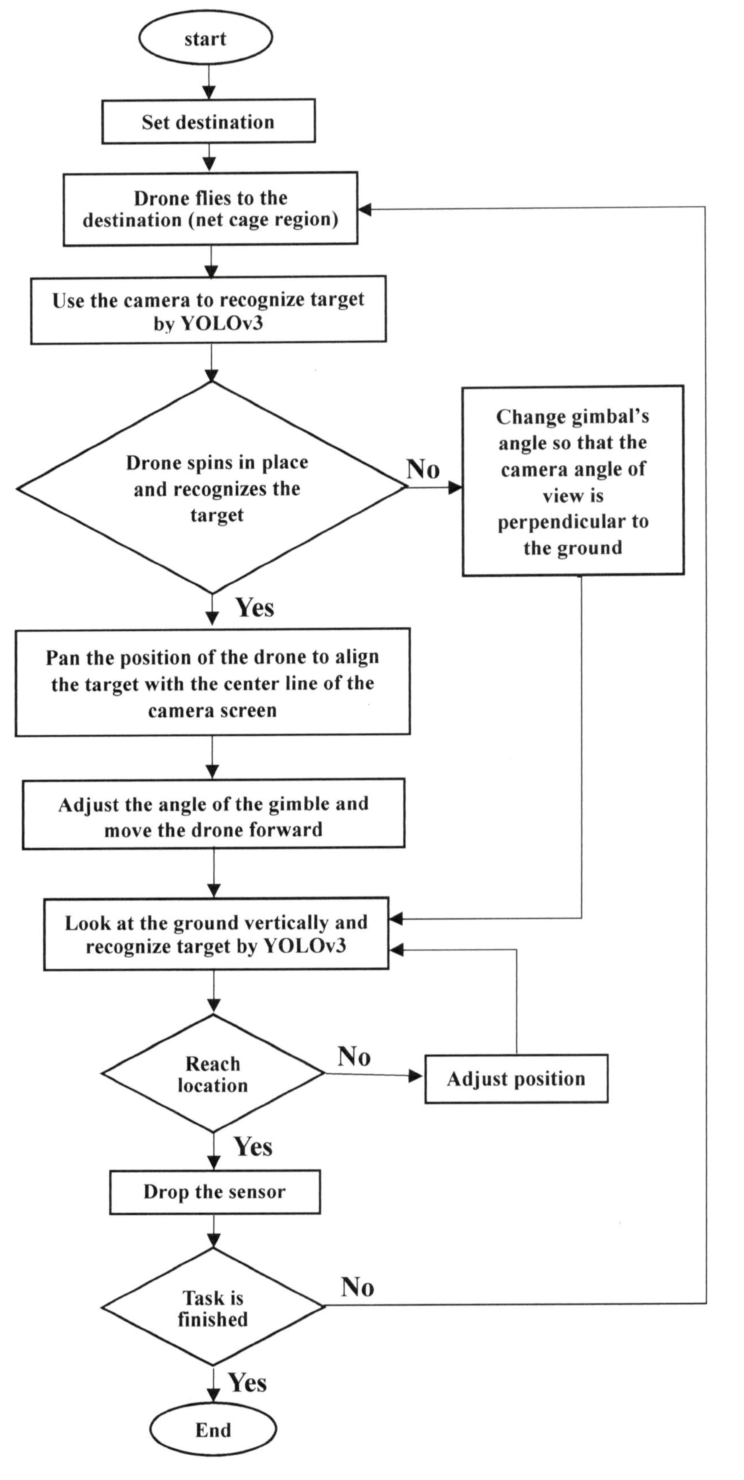
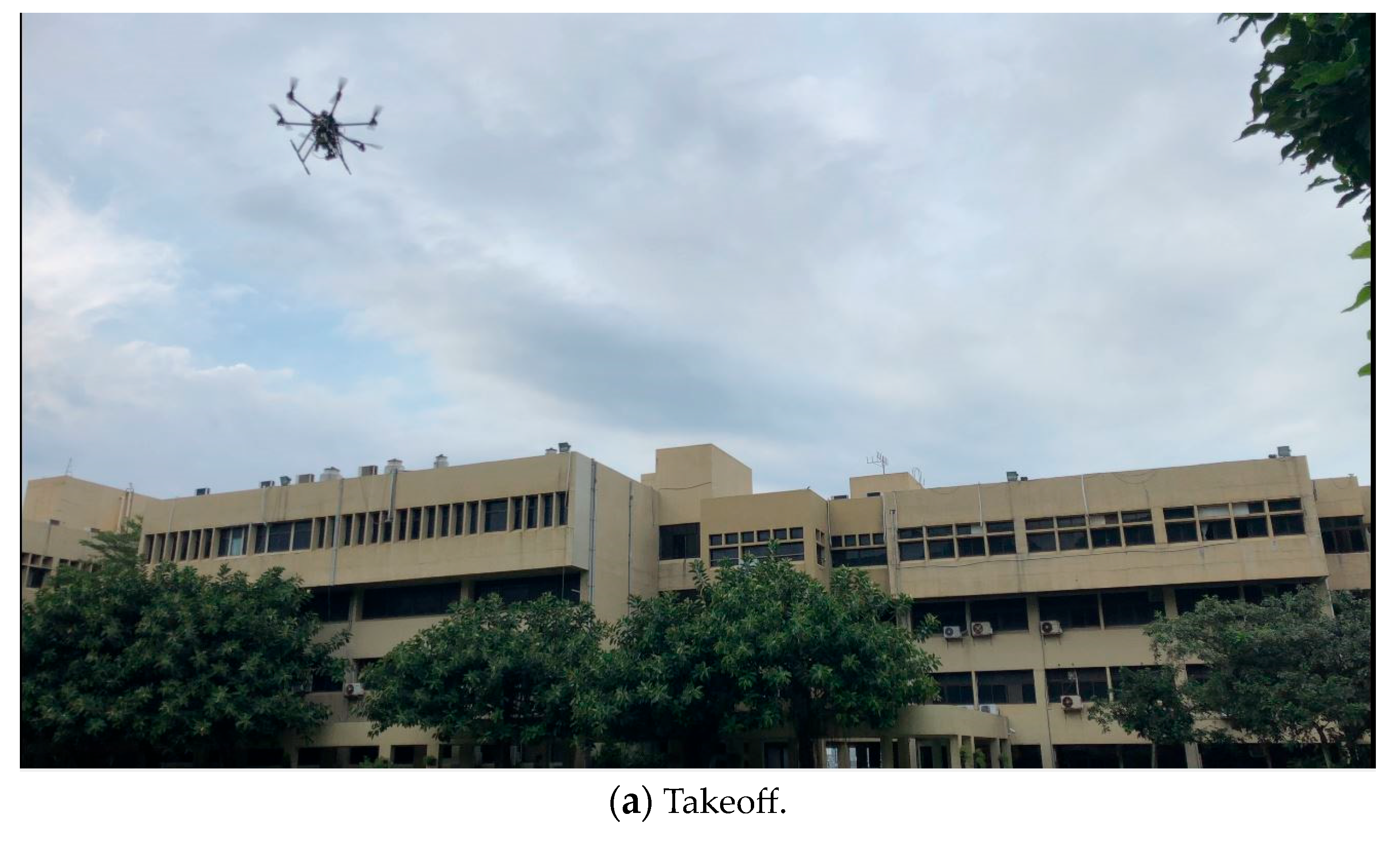
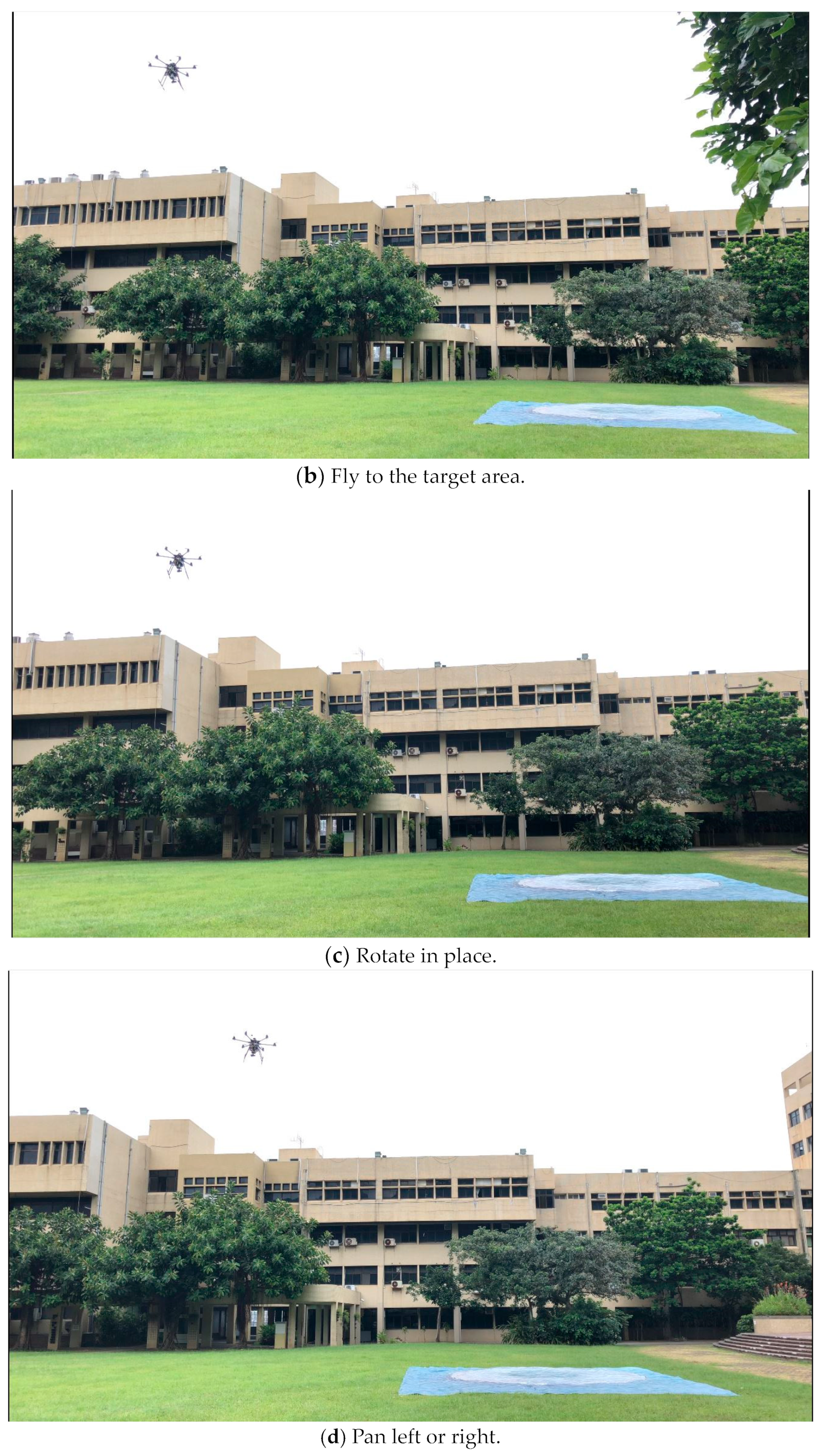
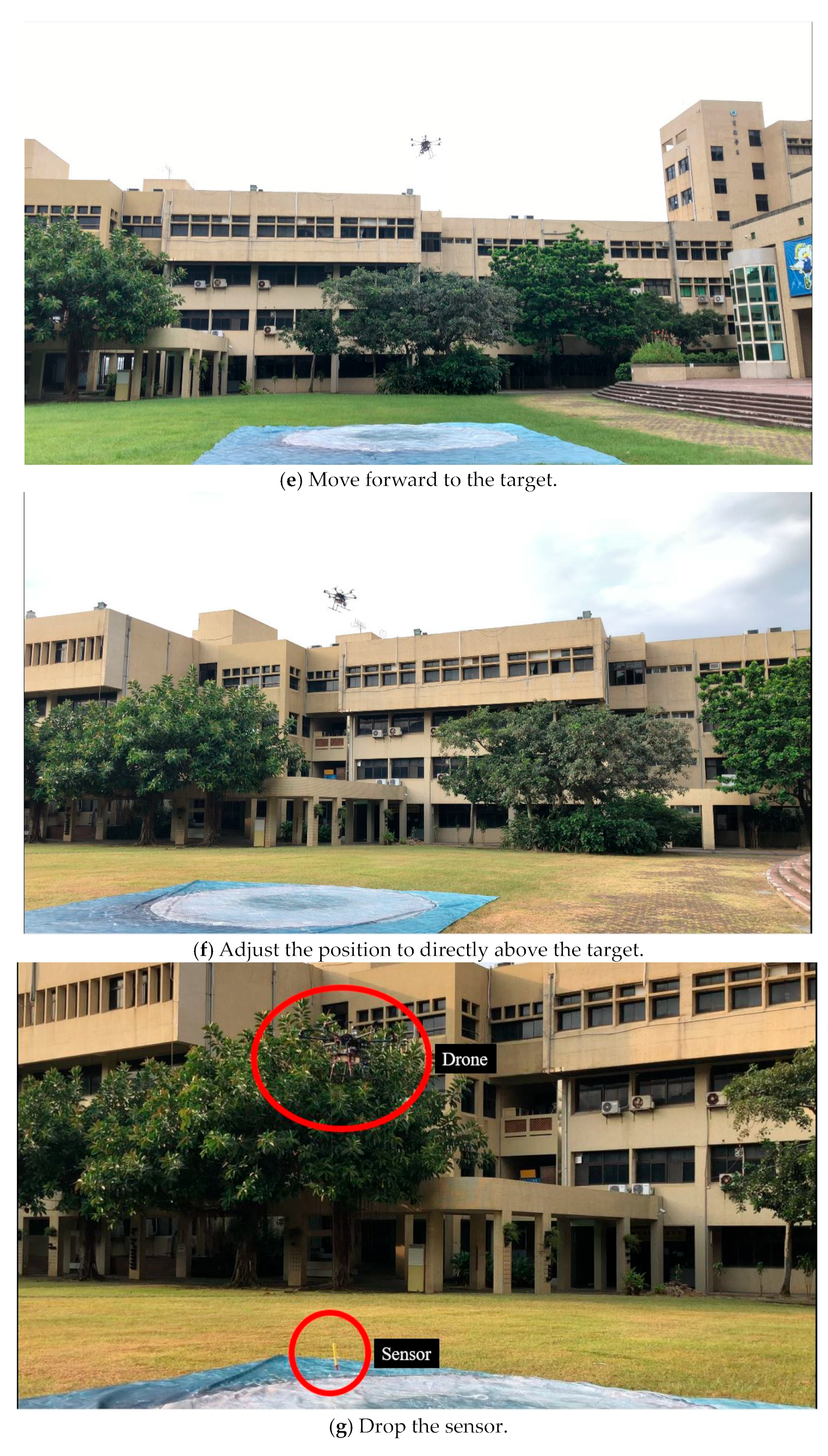
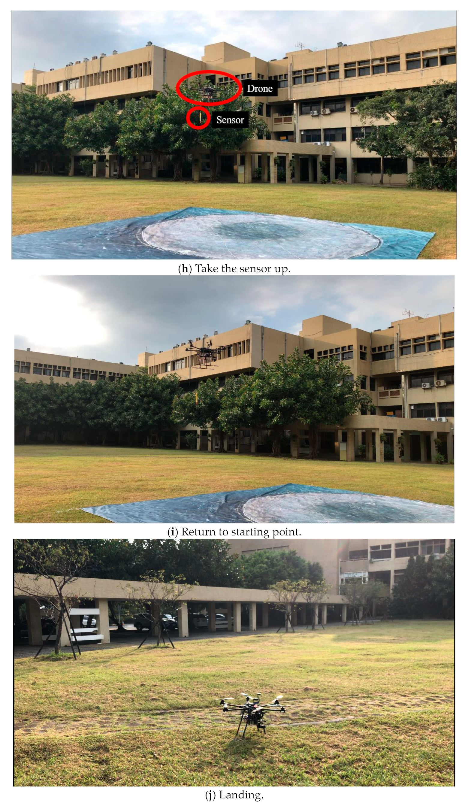
This study mainly uses image recognition and a UAV to assist net cage farmers. After the UAV cruises to its destination through GPS, the gimbal will be controlled; the camera will be used to identify the specified target, and the position of the UAV will be adjusted to the target. This experiment can correct the error caused by the difference in GPS quality. The average error of GPS is 1.7–2.3 m. After using the proposed scheme, the error can be reduced to 0.22–0.35 m. In the past, when deep learning was applied to flight vehicles, it was limited by hardware equipment, so the FPS and recognition rate could not reach the ideal state. For the weights to be trained, we mainly collect all aspects of the net cage. After that, the Jetson TX2 is selected to execute the modified network and control the UAV. We also use peripherals such as cameras, servo motors, and sensors for integration. Under normal circumstances, pattern recognition is affected by light when identifying a target. We collect as many target images as possible under different angles and different lights for training. This can increase the confidence score and mAP for the target identification. For the reduced filter model application part, the model using fewer filters has more opportunities to cause a recognition error of the target object, so when performing the task, we can choose the appropriate model. If it is a more straightforward target, we can select a model with fewer filters to reduce the amount of computing. In addition, when identifying moving targets, using a filter with less weight can increase the FPS and speed up the UAV’s reaction.

This study proposes a control scheme using UAV to solve environmental data collection and net cage detection in aquaculture. We integrate assembled UAV with the Jetson TX2, camera, servo motor, and sensor to enhance drone autonomy in aquaculture water quality measurement. Compared to commercial drones, we can adjust types of equipment and parameters according to requirements. The UAV uses a carry-on camera to recognize the specified target and fine-tune its position to reach the destination more accurately. UAV navigation errors from GPS are corrected using image assistance. Image recognition is applied to compensate for GPS errors and adjust the UAV position, ensuring the water measurement sensor can be accurately dropped into the destination net cage. Since the Yolov3 can be used to recognize more complex targets [32], it can be applied to the recognition of moving and complex targets in the future, or we can use an algorithm with lower accuracy and computational load, such as CenterNet [33]. The UAV can reduce the time and power consumption required for the mission. If we want a higher FPS, the Yolo-Lite [34] can be applied to improve the model. Identifying more straightforward targets can avoid misidentification and reduce the reaction time. In addition, when the drone flies forward because it relies on GPS positioning, there will be some distance and speed errors. Visual servo control can make corrections and make the movement more precise. This study used the Jetson TX2 to calculate the data in the development board. The number of CUDA of this development board computer is 256. The greater the number of CUDA, the faster the number of operations can support algorithms with more extensive procedures. In the future, the Jetson AGX Xavier, with a higher CUDA number, can be used with 512 CUDA, or we can use the Jetson Xavier NX, which has a lower number of CUDA but a lighter weight, with 384 CUDA.