Fluid–Structure Interactions between Oblique Shock Trains and Thin-Walled Structures in Isolators

Abstract

Understanding aeroelastic issues related to isolators is pivotal for the structural design and flow control of scramjets. However, research on fluid–structure interactions (FSIs) between thin-walled structures and the isolator flow remains limited. This study delves into the FSIs between thin-walled panels and the isolator flow, as characterized by an oblique shock train, by quantitatively analyzing 11 flow parameters assessing the structural response, separation zones, shock structures, flow symmetry, and performance. The results reveal that an FSI triggers panel flutter under oblique shock train conditions, with the panel shapes exhibiting a combination of first- and second-mode responses, peaking at 0.75 of the panel length. Compared to rigid wall conditions, isolators with a flexible panel at the bottom wall experience downstream movement of the separation zones and shock structures, reduced flow symmetry, and minor changes in performance. Transient fluctuations occur due to the panel flutter. Two flexible panels at the top and bottom walls have a comparatively lesser influence on the averaged parameters but exhibit more violent transient fluctuations. Furthermore, the FSI effects under oblique shock train conditions are contrasted with those under normal shock train conditions. The flutter response under normal shock train conditions is more pronounced, with a larger amplitude and higher frequency, driven by the heightened participation of the first-mode response. The effects of FSIs under normal shock train conditions on the averaged parameters are the opposite (with a larger influence) to those under oblique shock train conditions, with significantly more drastic transient fluctuations. Overall, this study sheds light on the complex and substantial influence of FSIs on the isolator flow, emphasizing the necessity of considering FSIs in future isolator design and development endeavors.

1. Introduction

The isolator serves as a pivotal component in scramjet engines, which are envisioned to power the next generation of hypersonic air-breathing flight vehicles [1,2]. Positioned between the hypersonic intake and the combustor, the isolator typically features a duct with either a rectangular or circular cross-section. Its primary function is to decelerate the incoming supersonic flow from the intake and to prevent the back-propagation of disturbances from the combustor to the inlet [3]. Extensive research has been dedicated to understanding the complex flow structures and mechanisms within the isolator [4,5,6], which are crucial for optimizing scramjet engine design and developing effective flow control strategies [7,8,9]. However, the aeroelastic challenges associated with the isolator have not received as much attention, despite their significant implications for the development of future hypersonic vehicles [10,11]. To address this gap, a series of numerical studies have been initiated, focusing on the effects of flexible structures on the isolator’s flow field and performance [12,13,14,15,16,17]. This research constitutes an integral part of these ongoing efforts.

Within the confined space of an isolator duct, the shock wave/boundary layer interactions (SBLIs) create a complex and unique flow phenomenon. When the shock is sufficiently strong to separate the boundary layer, it bifurcates and interacts with this separated layer [18]. The bifurcated shocks propagate downstream and are repeatedly reflected off the duct walls, forming a sequence of shocks followed by a region of adverse pressure gradients. This flow structure is known as a “shock train”. Experiments have identified two types of shock trains [19]: the “normal shock train” and the “oblique shock train”. The normal shock train typically begins with a bifurcated normal shock, followed by several non-bifurcated shocks. Conversely, an oblique shock train forms through the intersection of two leading oblique shocks, creating a series of “X” structures [5]. Each shock train type has distinct characteristics, largely influenced by the incoming Mach number. Oblique shock trains typically occur at higher Mach numbers and tend to be asymmetric, with the pattern adhering to one side of the isolator wall [19]. This pattern is found to be neutrally stable, with the shock system occasionally flipping from one wall to the other. In contrast, the normal shock train usually remains symmetric about the isolator’s centerline. Furthermore, the oblique shock train is less sensitive to the degree of flow confinement, which more significantly affects the length and spacing of consecutive shocks in the normal shock train [19,20,21]. Studies also indicate that the inherent unsteadiness of the oblique shock train is more pronounced than that of the normal shock train, with increases in the Mach number amplifying the shock fluctuation amplitude and leading to shock position displacements of up to one duct height at high Mach numbers [5,22,23].

In the context of aeroelasticity, the combination of extreme localized pressure loads induced by shock trains and the prevalent use of thin-walled panels in scramjet engine designs—due to the stringent lightweight requirements—inevitably trigger a pronounced fluid–structure interaction (FSI) response [14]. Additionally, the differing flow characteristics between the oblique and normal shock trains may precipitate distinct FSI features in the dynamic responses of structures and flow fields. Despite this, the potential FSI between thin-walled structures and shock trains has garnered relatively little attention. This oversight can be attributed to the nascent stage of scramjet engine technology development, which faces numerous challenges [3,4]. Much of the existing literature has concentrated on the integrated design of the intake and the body, the “start-up” procedures of the intake, intake surge, the effectiveness of the isolator, fuel mixing, and the stability of combustion. These factors collectively determine the feasibility of scramjets. In experimental tests, typically conducted at sea level, the operating duration of the engines is brief and the test model structures are rigid [24], thus minimizing the prominence of aeroelastic issues and resulting in a limited research focus.

As the scramjet technology is gradually applied to hypersonic flight vehicles, the significance of aeroelastic problems has been pointed out by many scholars [10,11,25]. The FSI between thin-walled panels and shock trains in isolators is essentially a unique form of panel flutter, where the structural response of the panel becomes unstable and undergoes limit cycle oscillation (LCO) beyond certain dynamic pressure thresholds [26,27]. Dowell [28] and Mei [29] have thoroughly examined and reviewed studies on the panel flutter in supersonic flow. Meng further investigated the nonlinearity of the aerodynamic responses caused by panel vibration [30,31] and panel flutter [32] in supersonic airflow. While the traditional mechanisms of panel flutter are well understood, investigations into the panel flutter induced by SBLI are still in the preliminary stages. Recent experimental work by Spottswood [33,34] and Willems [35,36,37] has identified strong evidence of mutual fluid–structural couplings and violent dynamic responses of panels under shock impingement. These experimental findings are supported by numerical studies by Visbal [38] and Ye [39,40], which indicate that the stability of the panel is significantly compromised in the presence of strong shock impingements, leading to the earlier onset of panel flutter. Furthermore, the inclusion of aerodynamic heating considerations is shown to further compromise the stability of flexible panels [41], resulting in greater deformations [34,42].

Moreover, recent studies have revealed that the FSI between thin-walled panels and the internal flow of isolators is considerably more complex. Meng’s studies [12,13] have demonstrated that forced structural vibrations significantly influence the flow structures and performance of the isolator. In this context, thin-walled plates were placed in an isolator with an incoming Mach number of 1.6 to investigate the FSI between the normal shock train and the thin-walled plates. The observed LCO of the plates resulted in the upstream movement of the normal shock train, compromising the flow symmetry and isolator performance [14]. In an inlet–isolator configuration, Ye [16] discovered that the fluid–thermal–structural interactions between the bottom wall and the flow cause larger structural deformations, peaking at the leading edge of the inlet lip. These deformations alter the shock wave structure near the lip, intensify the shock within the isolator, extend the length of the separated region, increase the temperature of the external wall, and ultimately reduce the total pressure recovery coefficient. Yao [43] proposed an aeroelasticity-based flow control method to mitigate the effects of undesirable shock oscillation due to downstream pressure perturbations. The results showed a reduction in the shock oscillation amplitude of about 50%, improving the aerodynamic performance of the supersonic intake. Liu [44] also explored a shock train control strategy based on the aeroelastic effects of a flexible plate, finding that the dynamics of the flexible plate are highly sensitive to the cavity pressure beneath the plate.

While previous studies primarily focused on the FSI between normal shock trains and thin-walled structures, the features of oblique shock trains differ from those of normal shock trains, potentially leading to different FSI responses. Therefore, this paper investigates and compares the FSI between the oblique shock train and thin-walled panels to that of the normal shock train. The remainder of this paper is organized as follows: Section 2 introduces and verifies the numerical method, Section 3 presents the computational configuration and numerical setups, Section 4 analyzes the features of the oblique shock trains in a rigid isolator, Section 5 investigates the influence of two forms of fluid–structure interactions on the oblique shock train, Section 6 compares the influence of thin-walled panels on the oblique and normal shock trains, and Section 7 draws some conclusions.

2. Numerical Method and Verification

This study utilizes a coupled CFD/CSD method, established within the ANSYS Workbench (19.0) [45]. This approach integrates a two-way fluid–structural coupling to accurately analyze the interactions between the fluid flow and the structural responses.

2.1. CFD Method

The three-dimensional (3-D) compressible Unsteady Reynolds-Averaged Navier–Stokes (URANS) equations are solved using the ANSYS CFX module to compute the aerodynamic loads. Previous research has demonstrated that the RANS approach effectively captures the mean flow structures of shock/boundary layer interactions (SBLIs), including in 3-D contexts [46]. This accuracy is attributed to the flow characteristics post-separation, which behave nearly inviscidly and rotationally away from the boundary surfaces. The conservation form of the governing equations can be expressed as:

$$\frac{\mathit{\partial }}{\mathit{\partial }t}{\displaystyle {\iiint }_{\Omega }\mathbf{Q}\mathrm{d}V}+{\displaystyle {\iint }_{\mathit{\partial }\Omega }{\mathbf{F}}^{\mathrm{c}}(\mathbf{Q})\cdot \mathbf{n}\mathrm{d}S}={\displaystyle {\iint }_{\mathit{\partial }\Omega }{\mathbf{F}}^{\mathrm{v}}(\mathbf{Q})\cdot \mathbf{n}\mathrm{d}S}$$

(1)

The implicit density-based solver with double precision is used to solve Equation (1), employing the k-ω SST turbulence model. The advection is handled by the high-resolution scheme, utilizing a second-order upwind approach. The transient behavior is modeled using a high-resolution transient scheme, which primarily applies the second-order backward Euler method, reverting to the first-order method as necessary to ensure solution boundedness. Additionally, the high-resolution option is selected for the turbulence numerics, which uses high-resolution advection and the high-resolution transient scheme.

A timestep of 10⁻⁵ s with 20 inner iterations per step is employed. The selection of the timestep aligns with previous investigations on FSIs between shock trains and panels [44], and its convergence has been rigorously established in our prior studies [15].

2.2. Coupled CFD/CSD Method

The governing aeroelastic equations for the flexible structures are given by:

$$\mathbf{M}\ddot{\mathbf{x}}+\left({\mathbf{K}}_{\mathrm{s}}(\mathbf{T})+{\mathbf{K}}_{\sigma }\mathbf{(}\mathbf{T}\mathbf{)}\right)\mathbf{x}=\mathbf{F}$$

(2)

where $\mathbf{x}$ is the displacement vector. $\mathbf{M}$ is the mass matrix. ${\mathbf{K}}_{\mathrm{s}}\mathbf{(}\mathbf{T}\mathbf{)}$ and ${\mathbf{K}}_{\sigma }\mathbf{(}\mathbf{T}\mathbf{)}$ represent the traditional stiffness matrix and the thermal stress stiffness matrix, respectively. $\mathbf{F}$ is the aerodynamic force obtained from the CFD solver. The dynamic responses of the structures are computed using the Transient Structures module, based on the Finite Element Method (FEM).

In the two-way coupling process, the fluid and structural calculations are conducted independently within each timestep, with multiple exchanges of information through the sub-iterations. Initially, the CFD solver computes the wall pressure distribution, which is then interpolated to the structural surface meshes via the fluid–structural interface. Following this, the CSD solver calculates the structural deformations. These deformations are then transferred back to update the CFD mesh through the fluid–structural interface, ensuring that the mesh deformation reflects the structural response. This continuous exchange allows for accurate modeling of the interaction dynamics, as detailed further in reference [16].

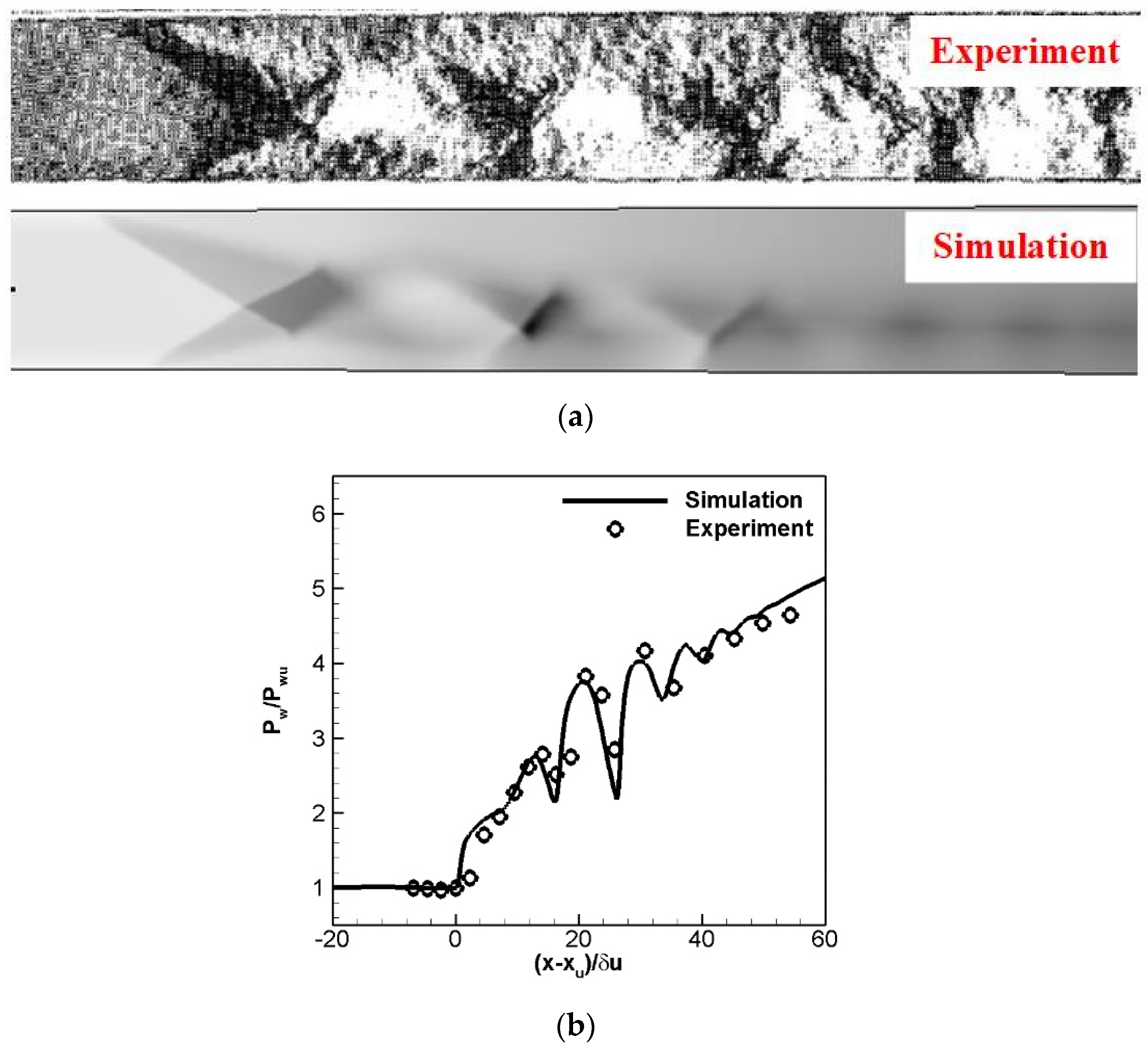
2.3. Verification Cases

• Verification of the CFD method

The CFD methodology is validated using the isolator experiment conducted by Carroll [19] as a benchmark case. Carroll’s setup involved experiments at two distinct incoming Mach numbers, M = 2.45 and M = 1.6, characterized, respectively, by oblique and normal shock trains. For this study, the Mach 2.45 case is simulated due to its relevance to oblique shock trains. The test section dimensions include a length of 754 mm and an inlet height of 38.1 mm, with both the top and bottom walls having a fixed divergence angle of 1.25 degrees. The boundary conditions, following the experimental setup detailed in [19], are summarized in

Table 1. Flow conditions for the verification case.

M	P0,in (kPa)	Tin (K)	Pout (kPa)t	T0,out (K)	δ (mm)	Re* (m−1)
2.45	309	134	107.5	295	3	$30\times {10}^6$

. P_0,in and T_in refer to the total pressure and static temperature at the inlet, respectively. P_out and T_0,out denote the static pressure and total temperature at the outlet, respectively. The inlet boundary layer, characterized by a thickness $\delta =3 \mathrm{m}\mathrm{m}$, is defined using the 1/7 power law velocity profile, a widely accepted approach in numerous studies [47,48].

The k-ω SST turbulence model is employed to simulate the behavior of shock trains in FSIs. Numerous studies [14,47,49] have demonstrated the wide application of the k-ω SST model in numerical investigations of isolator flow, accurately capturing the mean flow features and the large-scale motion of shock train structure, which are the interests of this paper. High-fidelity models like LES and DNS, though more precise, are computationally intensive and less feasible for extensive FSI simulations [50]. URANS is thus preferred for addressing aeroelastic and aerothermoelastic challenges in high-speed aircraft experiencing complex SBLIs [16,43,44]. The limitations of the computational resources and the complex nature of the FSIs between shock trains and flexible panels preclude the exploration of shock unsteadiness in this study.

For the verification case, the steady-state approach is employed. This choice was made because the unsteady simulation of the shock train flow at a fixed backpressure converges to a stable solution that is essentially the same as the steady-state solution. The steady-state approach can provide a consistent and reliable solution for the verification of our model. Figure 1a presents a comparison of the schlieren images from both the simulation and Carroll’s experiment, showing good alignment in the shock structure visualization. Additionally, Figure 1b displays the pressure distributions along the bottom wall where the oblique shock train is attached, further validating the simulation’s accuracy against experimental data. p_w represents the wall pressure. x_u and p_u are the x-coordinate and wall pressure at the location of the initial shock, respectively, and $\delta$ is the boundary layer thickness at the inlet.

2.

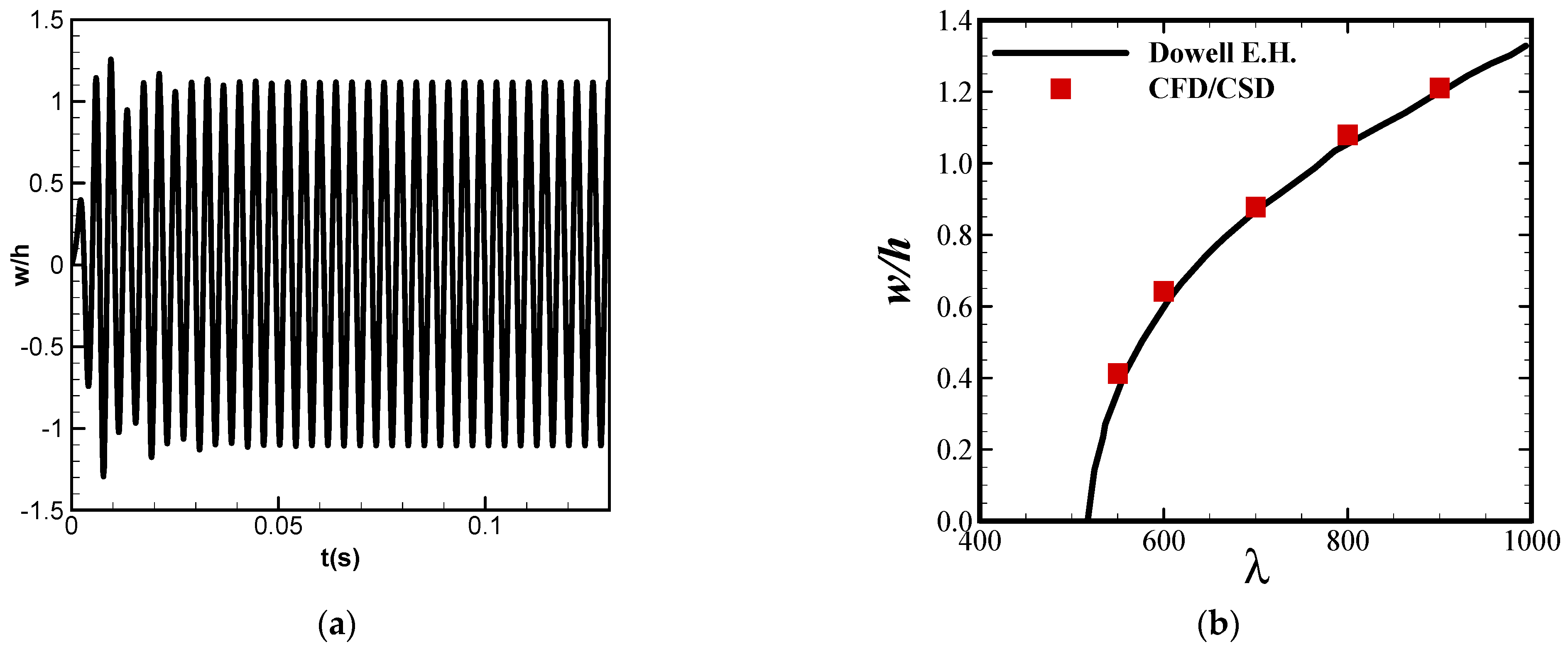
Verification of the coupled CFD/CSD method

The effectiveness of the coupled CFD/CSD methodology is demonstrated by simulating the aeroelastic behavior of a square panel with simply supported edges in a supersonic airflow [26,27]. The incoming Mach number and mass ratio are $M=2$ and $\mu /M=0.1$. The mass ratio is defined as $\mu =\rho l/{\rho }_{m}h$, where $\rho$ is the density of the freestream and ${\rho }_m$ is the density of the panel. The thickness ratio of the panel is denoted as $h/l=0.002$, where $h$ is the panel thickness and $l$ is the panel length.

Dowell’s research [26,28] indicates that panel instability and flutter initiate when the dimensionless dynamic pressure $\lambda$ ($\lambda =2q{l}^3/D$, $q$ is the dynamic pressure and $D$ is the panel stiffness) exceeds a critical value. The dynamic structural response is illustrated in Figure 2a at the position 0.75l (centerline), showcasing the LCO at λ = 800, with $w$ representing the displacement normal to the panel.

The validity of the coupled CFD/CSD method is further corroborated by comparing the numerical outcomes of this study with those obtained by Dowell, who employed a combination of Von Karman’s large deflection theory and the first-order piston theory. The comparisons, as illustrated in Figure 2b, show excellent agreement between the vibrational amplitudes at various $\lambda$, confirming the method’s capability to accurately predict the aeroelastic responses of thin-walled panels.

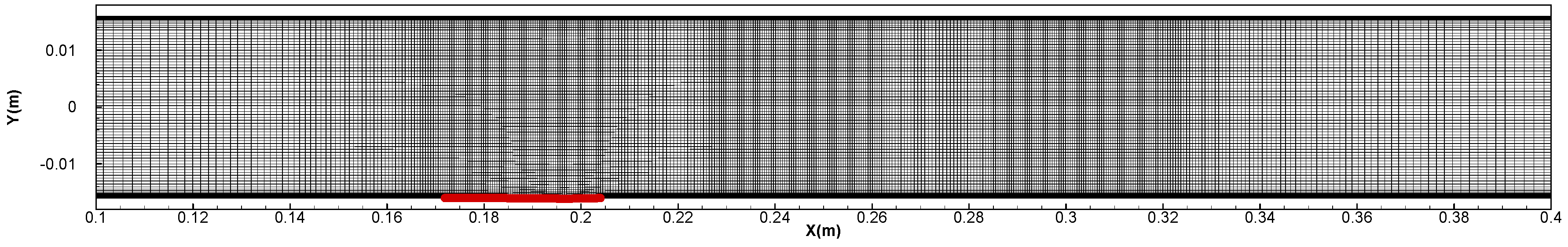
3. Computational Configuration and Setup

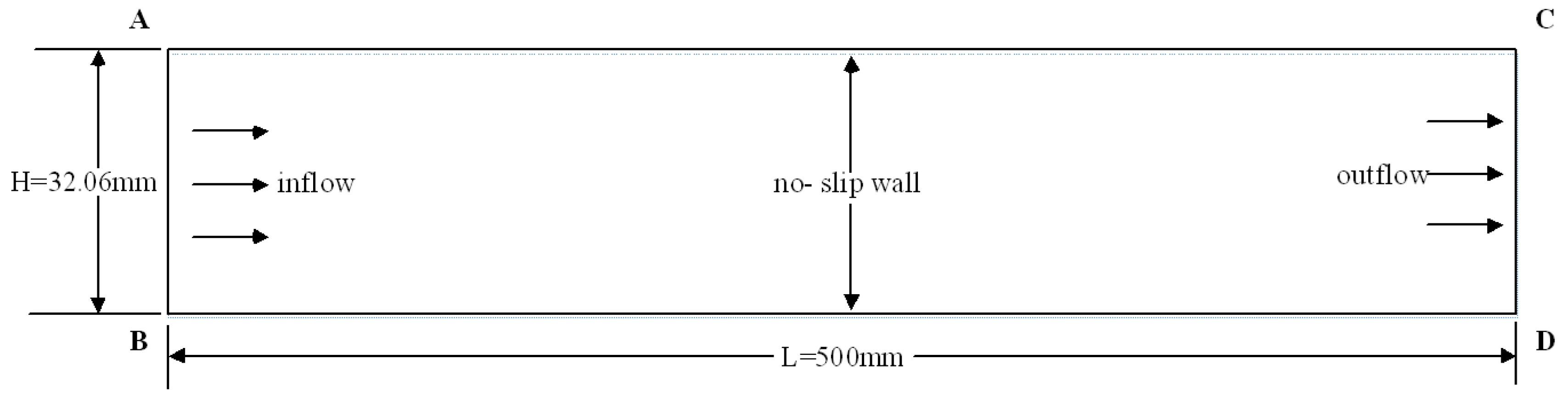
3.1. Computational Configuration

The numerical configuration of the isolator, as illustrated in Figure 3, is based on our previous research endeavors [12,13,14]. The computational configuration employs a 2-D isolator with a rectangular geometry that maintains a constant width. The domain has a length of 500 mm and a height of 32.06 mm, with no divergence between the top and bottom walls. At boundary AB, a supersonic inflow condition is imposed. The inlet boundary layer, characterized by a thickness δ = 3 mm, is defined using the 1/7 power law velocity profile, a widely accepted approach in numerous studies [47,48]. Boundary CD is specified as a pressure outlet, while AC and BD represent wall boundaries with no-slip and adiabatic conditions. The specific flow conditions utilized in the simulations are provided in

Table 2. Flow conditions.

M	P0 (KPa)	PAB (KPa)	PCD (kPa)	TAB (K)	TCD (K)	δ (mm)
2.45	309	48.5	285.5	195	295	3

.

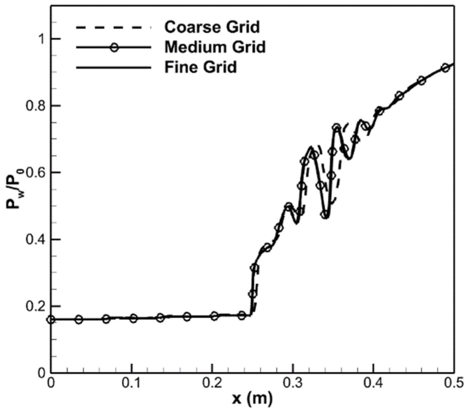
3.2. Grid Convergence Study

A grid convergence study is conducted to determine the optimal grid size for the simulation. Three grid configurations with 10,000, 50,000, and 100,000 cells are compared. The pressure distributions along the bottom wall, where the oblique shock train attaches, are compared in Figure 4. The pressure profiles between the medium and fine grids exhibit close alignment, whereas the coarse grid displays slight discrepancies. Considering both the computational accuracy and efficiency, the medium grid is chosen. Figure 5 illustrates the computational grid, with the red line representing the thin-walled panel, which will be elaborated upon in subsequent sections. To accurately capture the formation of the oblique shock train and the changes induced by panel flutter, grid refinement is implemented near the panel and the front of the shock train. The distance of the first grid to the wall is set to 0.01 mm, ensuring a $y^{+}$ value of approximately 1 near the panel and ensuring that $y^{+}$ remains below 5 for the entire wall.

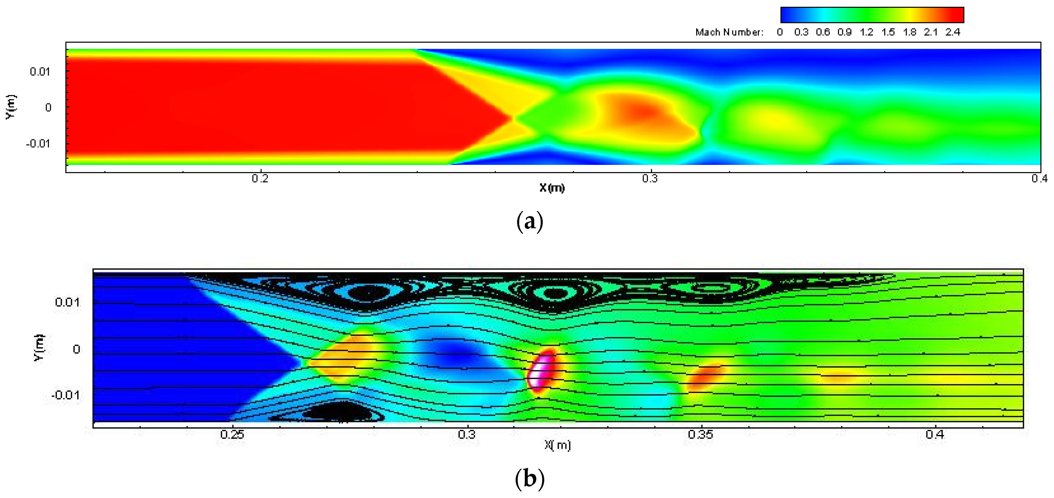
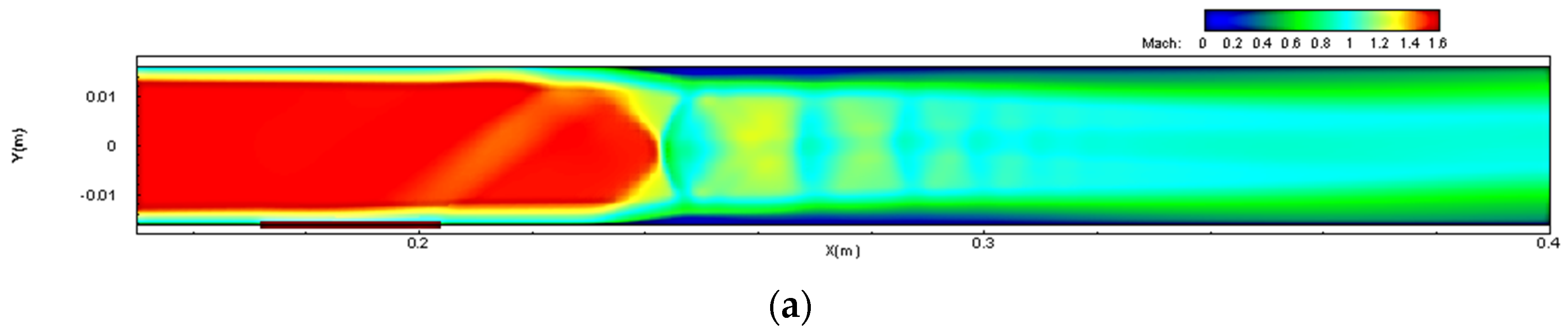
4. Flow Structures of Oblique Shock Train under Rigid Wall Conditions

To establish a benchmark, the flow structure of an oblique shock train in a 2-D rectangular isolator with rigid walls is simulated. As shown in Figure 6, the oblique shock train comprises oblique primary shock waves at the forefront, succeeded by a sequence of near-normal shocks with diminishing intensity and spacing. The initial shock in the train displays an asymmetric oblique shock pattern, evident in the Mach contour (Figure 6a). On both the top and bottom walls, boundary layer separation induced by the adverse pressure gradient is observed, giving rise to oblique shocks on both surfaces. Notably, the foot of the leading oblique shock on the top wall precedes that on the bottom wall. As these leading shocks intersect below the centerline, reflected shocks are generated.

Concurrently, the separation zones emerging behind the shock foot on both walls contribute to a throat-like geometry, akin to a virtual nozzle throat (Figure 6b). The interaction of the refracted shocks with the separated boundary layer leads to the formation of near-normal shock structures, fostering a primary compression region where the flow undergoes re-acceleration to supersonic velocities. This iterative process of shock interactions with the separated boundary layer engenders a succession of secondary shocks, perpetuating the sequence of flow decelerations and accelerations.

The oblique shock train manifests a distinct asymmetric pattern. The separation zone on the top wall, characterized by four consecutive separation bubbles (or vortex cores based on streamlines), markedly surpasses the corresponding zone on the bottom wall, which comprises only one separation bubble. Notably, the oblique shock train pattern exhibits a tendency to “lean” toward the bottom wall, a phenomenon often described as being “attached” to the bottom wall in the existing literature [19]. This pattern demonstrates neutral stability, with the shock system being capable of adhering to either wall or intermittently transitioning between walls [19].

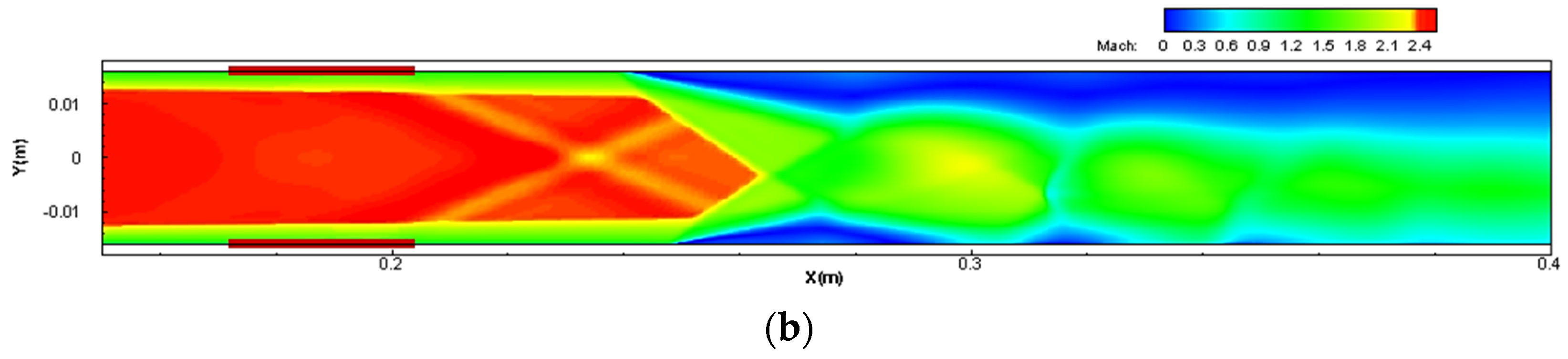
5. Influence of Thin-Walled Panels on Oblique Shock Train Structures and the Isolator Performance

5.1. The Structural Model of Thin-Walled Panels

To ensure consistency with our prior research [14], the same structural model for the thin-walled panel is adopted. As depicted in Figure 7, two aeroelastic cases are devised, each involving panels positioned differently. In Case 1, a single panel is placed solely on the bottom wall, whereas in Case 2, two panels are positioned on both the top and bottom walls. These panels, acting as adiabatic walls, are simply supported on both ends. The center of all the panels is located at $x=188 \mathrm{m}\mathrm{m}$, and the length of the panels is $l=32.06 \mathrm{m}\mathrm{m}$. The panel thickness ratio is $h/l=0.0031$ (this ratio is chosen around 0.002 in many studies regarding panel flutter [38,51]). The panels are made of structural steel with a Young’s modulus of $2\times 10^{11}$ and a Poisson’s ratio of 0.3. In the structural analysis conducted using ANSYS Workbench, shell elements are employed to model the panels, necessitating only one element in the thickness direction. The spanwise discretization involves 50 elements, ensuring adequate resolution for accurate simulations.

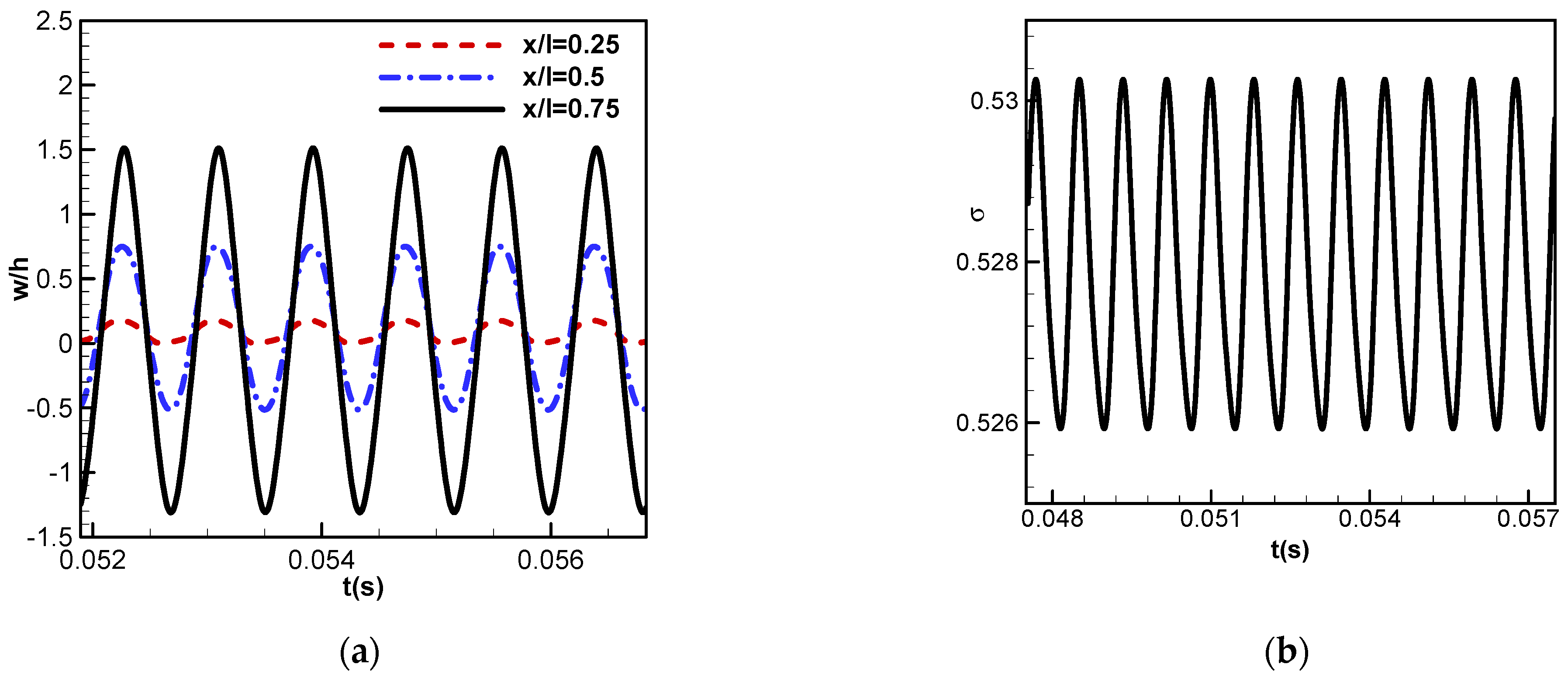
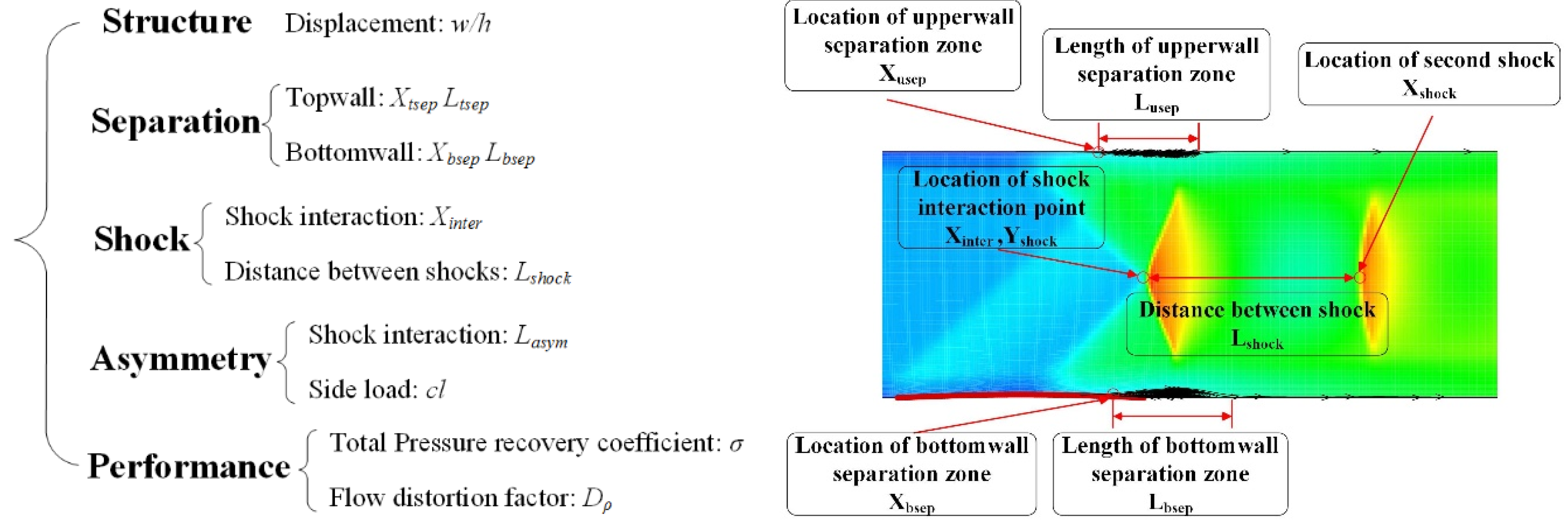
5.2. Definitions of Monitored Parameters

The dynamic responses of the structural and flow parameters in the FSIs for Case 1 and Case 2 are shown in Figure 8 and Figure 9, respectively. w is the structural displacement in the Y direction, and h is the panel thickness. $\sigma$ represents the total pressure recovery coefficient at the isolator outlet. The labels “top” and “bot” in the legend of Figure 9a correspond to the panels at the top and bottom walls in Case 2. In Figure 8a and Figure 9a, all the points on the panels exhibit oscillations with a fixed vibration amplitude and frequency, indicative of panels undergoing LCO in both cases. Concurrently, the flow field experiences periodic oscillations due to panel flutter, evidenced by the transient response of the pressure recovery coefficient in Figure 8b and Figure 9b. Consequently, both panel structures and flows exhibit periodic variations due to FSIs.

To quantify the influence of FSIs on the periodic fluctuations of the panel structures and the isolator flow, 11 parameters are defined and monitored in this paper. These parameters are classified into five categories: “Structure”, “Separation”, “Shock”, “Asymmetry” and “Performance”. The definitions of these parameters are presented in the schematic diagram depicted in Figure 10.

The “displacement” parameter signifies the structural response of the panel, calculated using the dimensionless structural displacement ($w/h$) at 0.75l of the panel.

The “Separation” and “Shock” parameters delineate the local flow structures of the oblique shock train. The “Separation” parameters encapsulate the characteristics of the separation zones, which are deemed critical sources of flow unsteadiness. Changes in their location and length can significantly influence the flow structures and isolator performance. The location of the separation zones is defined as the start of the separation bubbles, while their length is defined as the length of the separation bubbles. Denoted as $X_{t,sep}$, $L_{t,sep}$, $X_{b,sep}$ and $L_{b,sep}$, respectively, they represent the location and length of the separation zones at the top and bottom walls. The “Shock” parameters describe the characteristics of the oblique shock train structures. The shock intersection point marks the location where two oblique shocks meet and serves as the onset of the shock train. The $X$ coordinate of the shock intersection point is defined as the location of the first shock ($X_{shock})$, while the length between the first two shocks is denoted as $L_{shock}$.

The “Symmetry” parameters denote the flow symmetry level, crucial for mitigating undesirable large side loads and structural damage. Two parameters are included in the item “Symmetry”: the local flow symmetry factor L_sym, representing the local flow symmetry level at the front of the shock trains, and the lift coefficient $cl$, quantifying the overall flow symmetry level.

L_sym is defined as:

$$L_{sym}=\frac{Y_{shock}-Y_{center}}{H}$$

(3)

where $Y_{shock}$ is the $Y$ coordinate of the shock intersection point. $Y_{center}$ is the $Y$ coordinate of the isolator centerline (0 mm). $H$ is the height of the isolator.

$cl$ is defined as:

$$cl=\frac{F^{\prime }}{q_{\infty }l}$$

(4)

where $F^{\prime }$ is the side load per unit span and $q_{\infty }$ is the dynamic pressure of the flow at the isolator inlet.

The “Performance” parameters assess the overall isolator performance through two metrics. The total pressure recovery coefficient ($\sigma$) measures the isolator’s ability to recover the total pressure. The flow experiences total pressure loss when passing through the shock train, which indicates an undesirable phenomenon of energy loss. A larger total pressure recovery coefficient implies lesser total pressure loss. $\sigma$ is defined by:

$$\sigma =\frac{{\int }_{outlet}{P}_{0,oulet}dA}{{\int }_{inlet}\rho u{P}_{0,inlet}dA}$$

(5)

where $\rho$, $u$, and $P_0$ are the local density, velocity and total pressure, respectively. The numerator is the area fraction for the flow parameters at the outlet, while the denominator is the area fraction for the flow parameters at the inlet. The flow distortion index $D_{\rho }$ examines the uniformity level of the flow at the outlet. Due to the complex SBLIs inside the isolator, the uniform incoming flow at the inlet is distorted and becomes non-uniform at the outlet. Flow distortion is an undesirable phenomenon that compromises the performance of the combustion chamber. A larger flow distortion index implies more non-uniform flow. The flow distortion index can be calculated by:

$$D_{\rho }=\frac{{\rho }_{\max }-{\rho }_{\min }}{{\rho }_{ave}}=\frac{{\rho }_{\max }-{\rho }_{\min }}{\frac{{\displaystyle {\int }_{outlet}\rho u·\rho dA}}{{\displaystyle {\int }_{outlet}\rho udA}}}$$

(6)

where ${\rho }_{\max }$ and ${\rho }_{\min }$ are the maximum and minimum densities at the outlet, and ${\rho }_{ave}$ is calculated by the mass flow-averaged density.

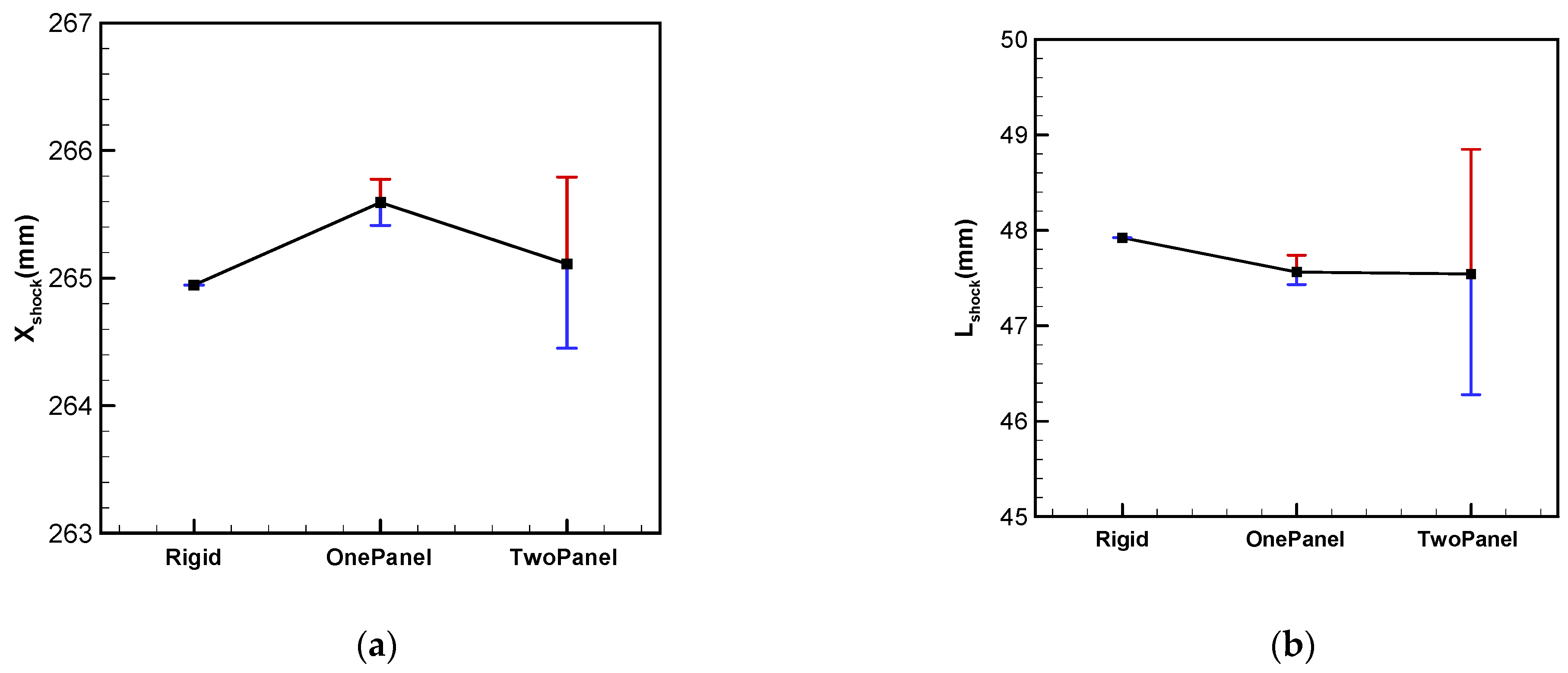
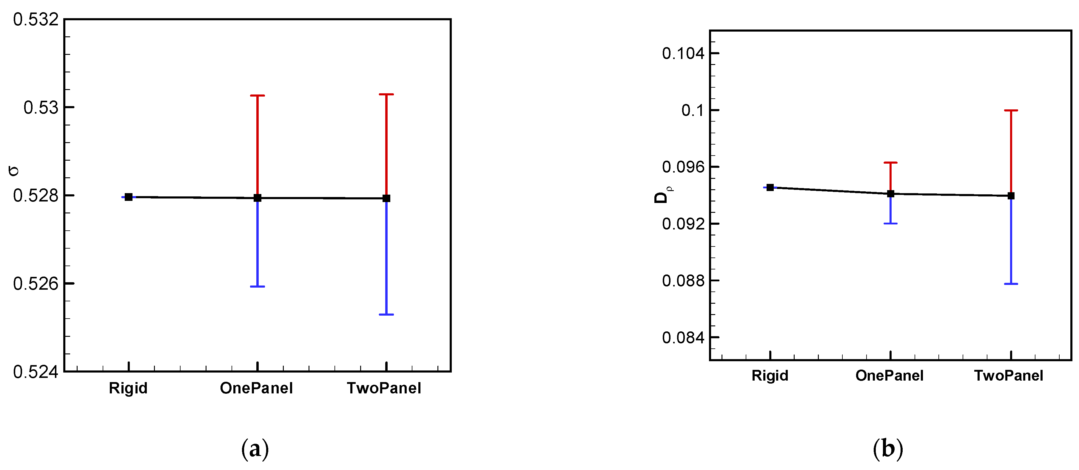
5.3. Analysis of the Influence of the Thin-Walled Panel

In Case 1, depicted in Figure 8a, the FSI between the thin-walled panel at the bottom wall and the internal flow of the isolators results in the flutter response in the panel structures. As depicted in Figure 7a, shocks and expansions arise due to the structural deformation of the panel, propagating downstream to interact with the oblique shock train structures, potentially altering the entire flow field.

In Case 2, the FSI triggers the flutter response of both panels. The panels at the top and bottom walls oscillate with the same frequency but an opposite amplitude, as observed in Figure 9a. Figure 7b illustrates that the induced shocks and expansions occur at both panels due to structural deformation. These induced phenomena cross near the isolator center line upstream of the shock train, generating refracted shocks that complicate the internal flow structures in the isolator.

To precisely compare the effect of the FSIs in both cases, the changes in the 11 parameters are monitored and analyzed.

• Structure

Figure 11a–c display the panel shape during one complete LCO for all the cases. In the legend, “OnePanel” represents the panel at the bottom wall in Case 1, “(TwoPanel)_top” represents the panel at the top wall in Case 2, and “(TwoPanel)_bot” represents the panel at the bottom wall in Case 2. Interestingly, despite the different deployment methods, the panel deflection shapes are quite similar. For Case 1 in Figure 11a, the panel shape resembles a combination of first- and second-mode responses, with the maximum deflection at 0.75l. In Figure 11b, the deflection shape of the panel at the bottom wall in Case 2 is similar to the panel shape in Case 1. The panel shape at t = T/4 and t = T of the panel at the bottom in Case 2 is almost the same as that in Case 1, while the panel shapes at other intermediate times show slight differences. Moreover, the panel at the top wall in Case 2 exhibits identical deflection to the bottom wall panel but in opposite directions.

Furthermore, Figure 11c compares the change in the structural displacement at 0.75l for the rigid wall condition, Case 1, and Case 2. On the X-axis, “Rigid” denotes the rigid wall condition, “OnePanel” denotes the panel at the bottom wall in Case 1, “(TwoPanel)_t” denotes the panel at the top wall in Case 2, and “(TwoPanel)_b” denotes the panel at the bottom wall in Case 2. The black line represents the average value, which is calculated by the weighted average value over five vibration periods. The red bar represents the maximum value during the vibration, while the blue bar represents the minimum value during the vibration. After reaching the LCO, all the panels flutter around the equilibrium position $w/h=0$ for Case 1 and Case 2. The flutter amplitudes of all the panels are 1.41h, and the flutter frequencies are 1215 Hz.

2.

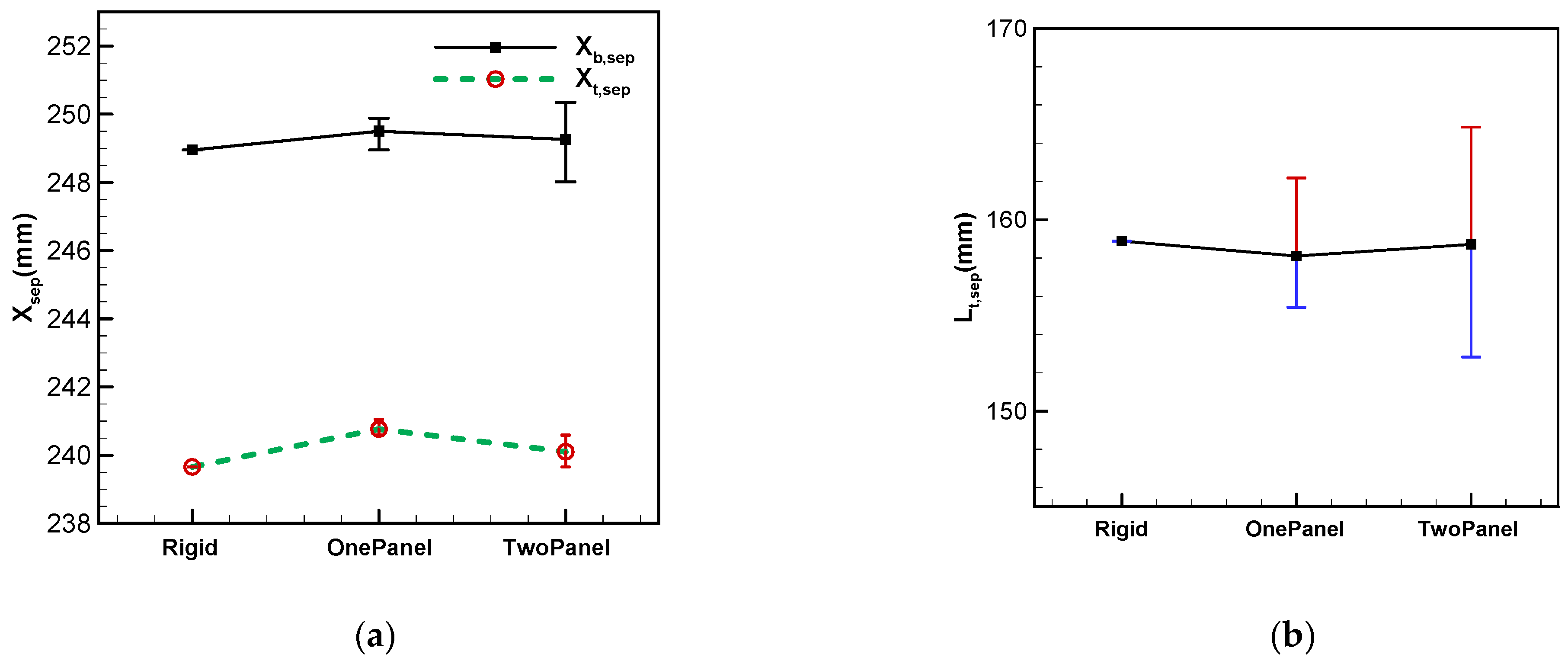
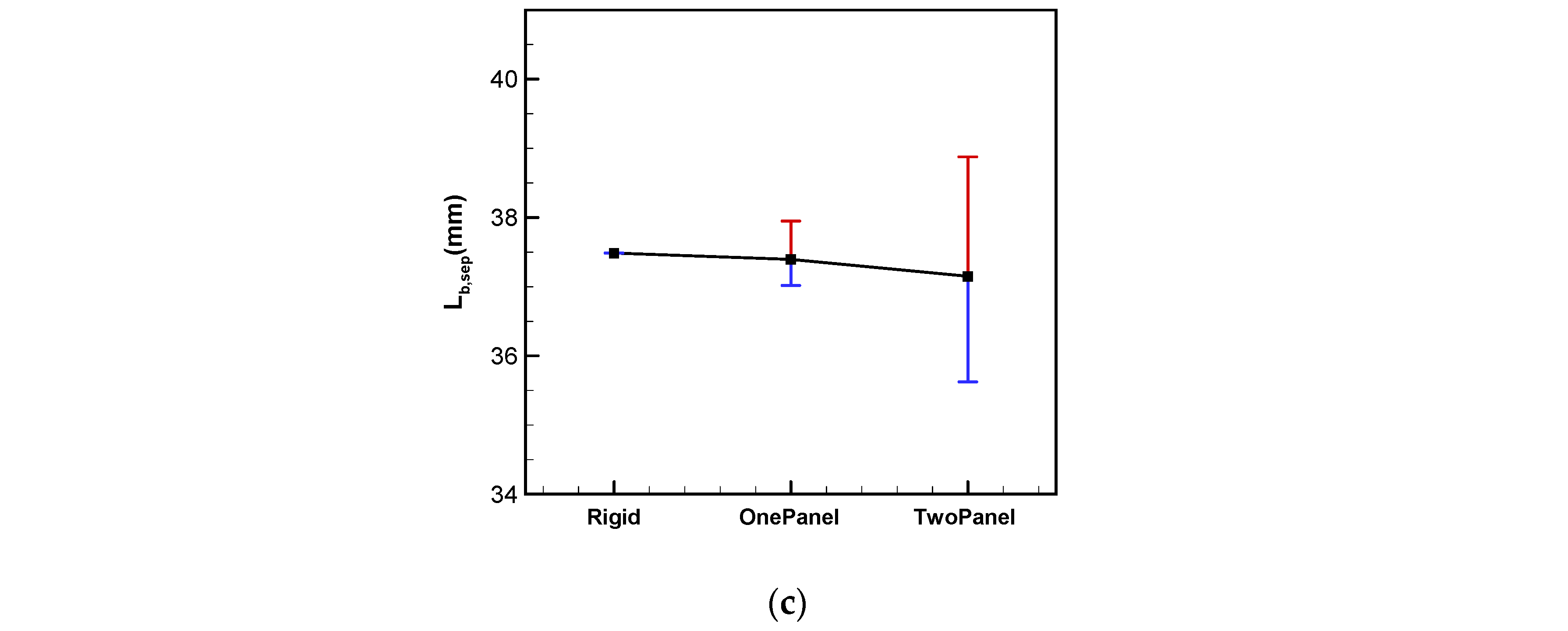
Separation

A comparison of the separation zone characteristics under rigid wall conditions, Case 1, and Case 2 is depicted in Figure 12. The black line represents the average value, while the red and blue bars indicate the transient maximum and minimum values, respectively. The separation zones at the top wall are notably larger and located upstream compared to those at the bottom wall. In Case 1, when the panel flutters, the separation zone at the top wall slightly moves upstream with reduced length. In Case 2, with fluttering of both panels, the separation zone at the top wall moves further upstream but remains downstream of the rigid wall conditions. The separation length increases compared to Case 1, yet it remains slightly shorter than the rigid wall conditions. The fluctuations in Case 2 are more pronounced than in Case 1.

Due to the unsymmetrical nature of the oblique shock train, the characteristics of the separation zones at the top and bottom walls are quite different. For all three conditions, the separation zones at the top wall are located upstream of the separation zones at the bottom wall, as shown in Figure 12a. Additionally, the lengths of the separation zones at the top wall are significantly larger than the separation zones at the bottom wall, as can be seen by comparing Figure 12b,c. This conclusion is also supported by the streamlines in Figure 6b. The separations zone at the top wall consists of four flattened separation bubbles, while the separations zone at the bottom wall only consist of one separation bubble.

For the separation zones at the bottom wall, in Case 1, the locations travel upstream with reduced length during panel flutter. In Case 2, similar upstream movement is observed, with a further decrease in the separation length compared to Case 1. The fluctuations in Case 2 are more pronounced, particularly at the top wall, indicating the larger influence of the FSI on the separation zone characteristics.

3.

Shock structures

Figure 13 compares the shock structures of the rigid wall conditions, Case 1, and Case 2. The black line represents the average value, while the red and blue bars indicate the transient maximum and minimum values, respectively. The front of the oblique shock trains, determined by the location of the first shock, slightly shifts downstream when the bottom wall panel flutters in Case 1 (Figure 13a) compared to the rigid wall conditions. In Case 2, the shock train location falls between the rigid wall conditions and Case 1. Additionally, the fluctuations of the shock train in Case 2 are more pronounced than in Case 1. The length of the oblique shock train, indicated by the distance between the first two shocks (Figure 13b), decreases slightly in Case 1 compared to the rigid wall conditions. In Case 2, although the average distance remains similar to Case 1, the transient fluctuations are more pronounced.

4.

Flow symmetry

The flow symmetry levels of the rigid wall conditions, Case 1, and Case 2 are compared in Figure 14. The black line represents the average value, while the red and blue bars indicate the transient maximum and minimum values, respectively. All the l_sym values are negative, indicating a tendency for the oblique shock train front to attach to the bottom wall, which can be seen in Figure 6 and Figure 7. Compared to the rigid wall conditions, the average l_sym magnitude decreases in Case 1 and further decreases in Case 2. The fluctuations in l_sym are more pronounced in Case 2, suggesting the greater influence of two thin-walled panels compared to one. However, the average lift coefficient values remain around zero for all the cases, with small transient fluctuations for Case 1 and Case 2, indicating the minor influence of the FSI on the overall flow symmetry.

5.

Performance

The comparison of the total pressure recovery coefficient for the rigid wall conditions, Case 1, and Case 2 is illustrated in Figure 15a. The black line represents the average value, while the red and blue bars indicate the transient maximum and minimum values, respectively. Under rigid wall conditions, $\sigma =0.528$. The average total pressure recovery coefficients for Case 1 and Case 2 are similar to the rigid wall conditions, with minor transient fluctuations. The fluctuations in Case 2 are slightly larger than in Case 1. Figure 15b illustrates the comparison of the flow distortion indices among the rigid wall conditions, Case 1, and Case 2. Compared to the rigid wall conditions, the average $D_{\rho }$ decreases slightly in Case 1 and further in Case 2. However, these changes are minor. Transient fluctuations in both cases are evident, with Case 2 exhibiting more pronounced fluctuations than Case 1.

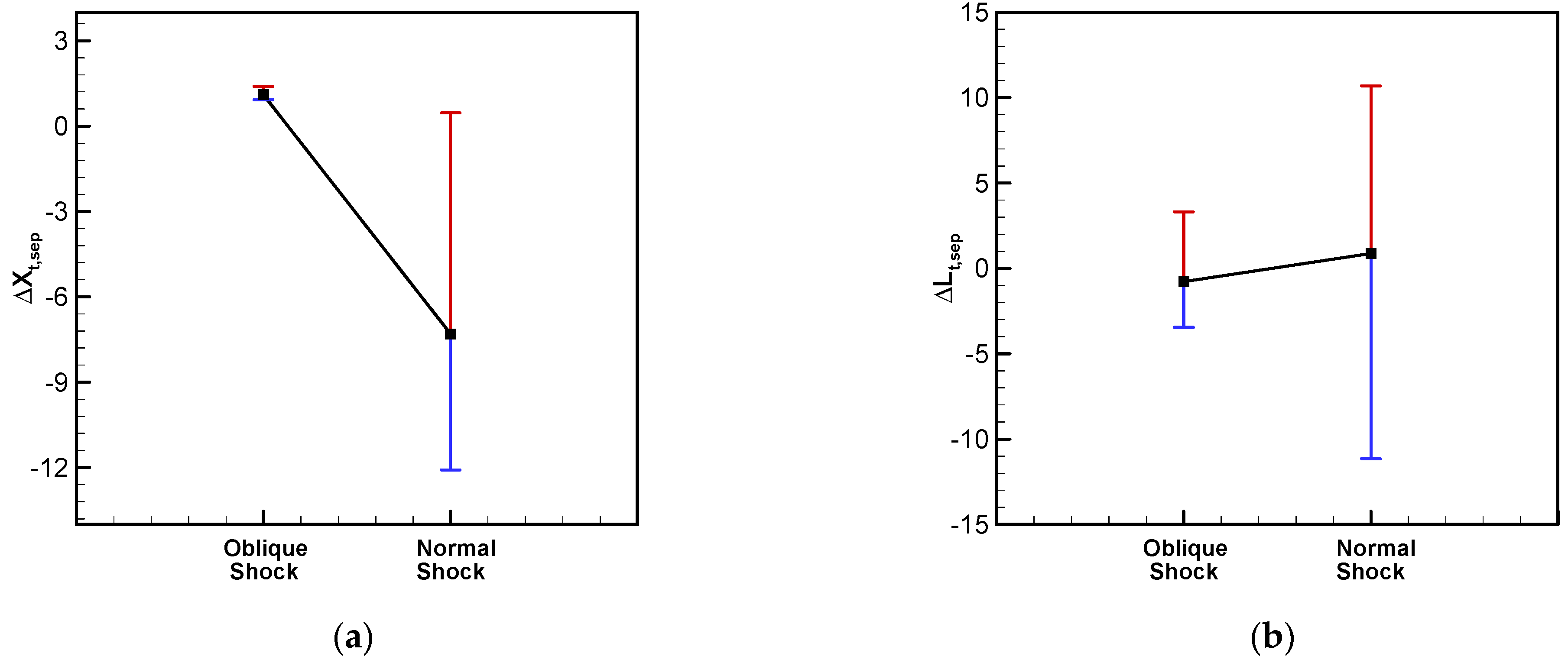
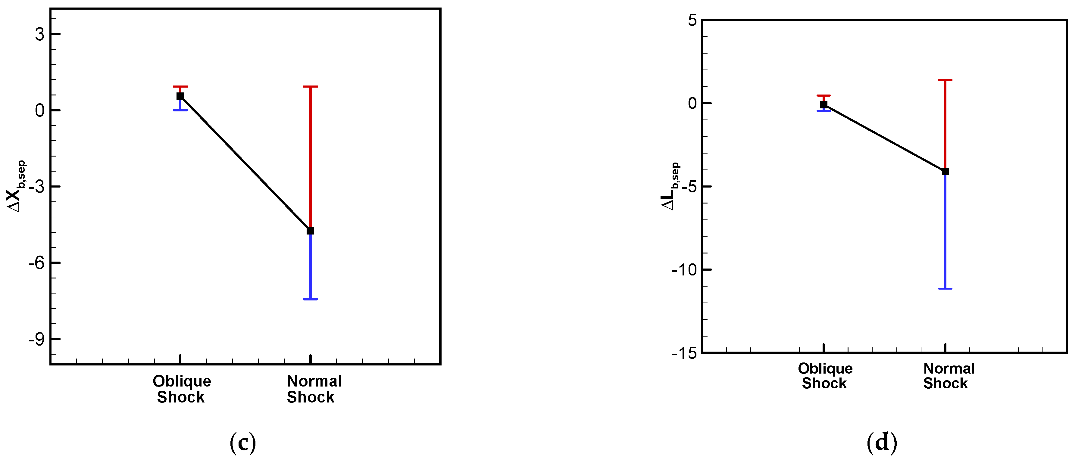
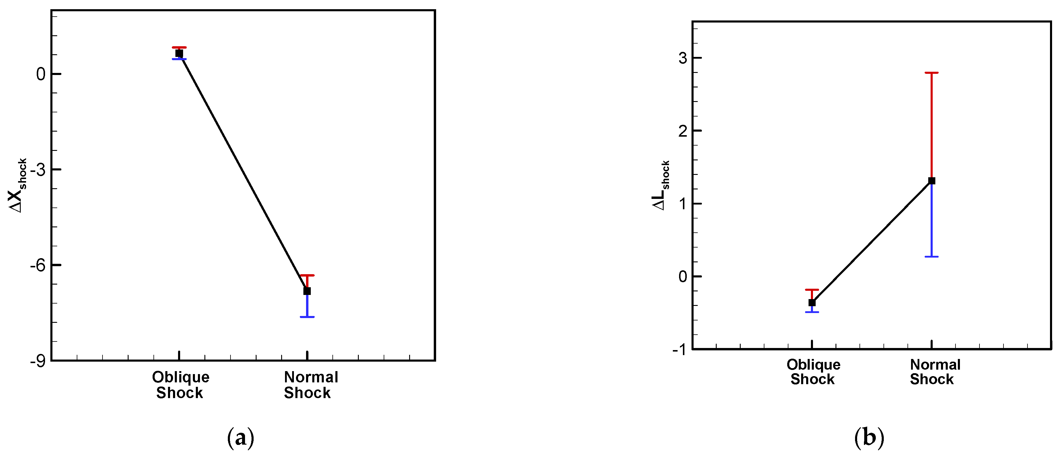
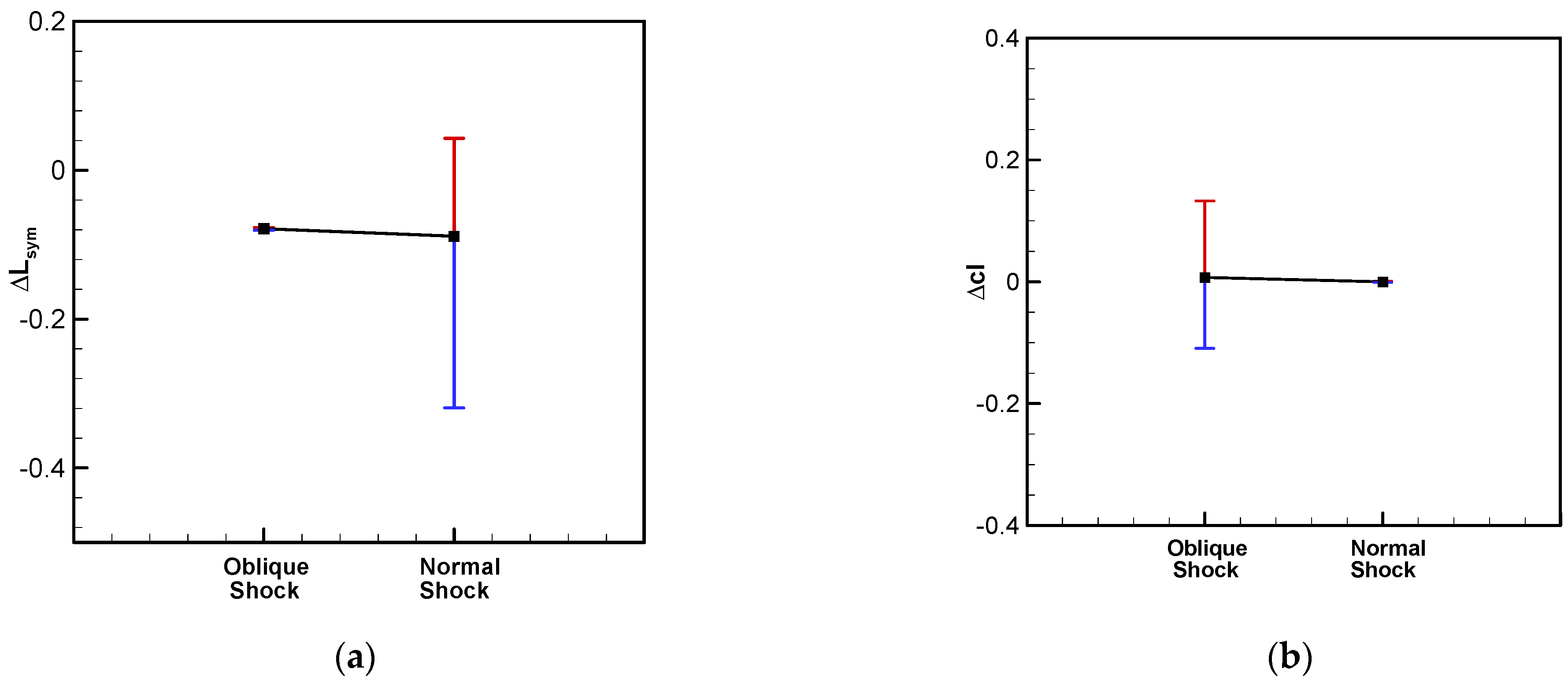
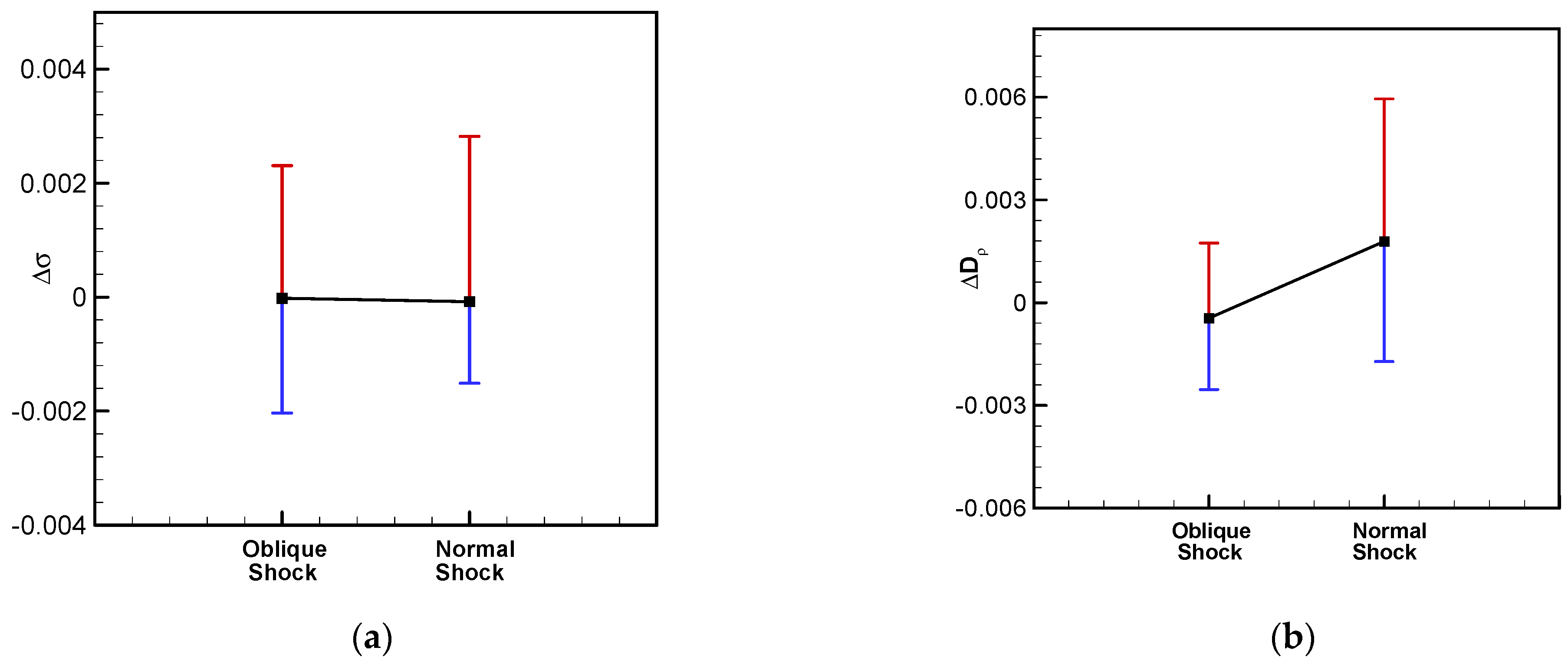
6. Comparisons of the Influence of Thin-Walled Panels on Oblique and Normal Shock Trains

In our previous work, the influence of the thin-walled panel on the normal shock train was investigated. Our analyses showed that the FSIs between the thin-walled panel and the internal flow of the isolators also led to the LCO of the panel structures. Consequently, the normal shock train also exhibited periodic oscillations, affecting the separation zones, shock structures, flow symmetry levels, and isolator performance.

This section compares the influence of thin-walled panels on oblique and normal shock trains by analyzing the parameters defined in Section 5.2. The isolator configuration for the normal shock train flow remains identical to that depicted in Figure 3, with the boundary conditions provided in

Table 3. Flow conditions of the normal shock train.

M	P0 (KPa)	PAB (KPa)	PCD (KPa)	TAB (K)	TCD (K)	δ (mm)
1.6	206	48.466	195.106	195	295	3

. Only one thin-walled panel is placed at $x=188 \mathrm{mm}$, upstream of both the normal and oblique shock trains, consistent with the panel structural model defined in Section 5.1.

Figure 16 compares the Mach contours of the flow field of the normal shock train and the oblique shock train influenced by the thin-walled panels. In both cases, the induced shocks and expansions at the panel due to structural deformation propagate downstream, interacting with the respective shock trains. However, due to the distinct shock train features, the FSI effects on normal and oblique shock trains may differ.

• Structure

Figure 17a illustrates the panel shape variations during one LCO period under normal shock train FSIs. Compared to the oblique shock train FSIs, the panel shapes under normal shock train conditions exhibit a more dominant first-mode response, with the maximum deflection occurring at approximately 0.65l. This discrepancy in the panel shapes is attributed to the Mach number’s significant influence on thin-walled panel dynamics [52]. In the low supersonic range, the first-mode response prevails, while higher supersonic regions show a more even participation of the first- and second-mode responses.

To compare the structural displacement under the normal and oblique shock train conditions, Figure 17b compares the changes in the structural displacement at 0.75l. On the X-axis, “Oblique shock” represents the FSI between the thin-walled panel and the oblique shock train, and “Normal shock” represents the FSI between the thin-walled panel and the normal shock train. The black line represents the average value, which is calculated by the time-averaged value over five vibration periods. The bars represent the minimum and maximum values during the vibration. Although both panels oscillate around the same equilibrium position $w/h=0$, the panels under normal shock train conditions exhibit significantly larger flutter amplitudes than those under oblique shock train conditions. The last three columns provide the specific amplitude values, indicating a greater intensity of vibration under normal shock train conditions. “Vibration amplitude” denotes the fluctuation amplitude of the parameters listed in the first column, “(Amp)_O” represents the vibration amplitude of the parameters for the FSI under the oblique shock train conditions, “(Amp)_N” represents the vibration amplitude of the parameters for FSI under the normal shock train conditions, and “R_amp” is calculated by (Amp)_O/(Amp)_N to compare the intensity of the vibration under the two conditions. Additionally, the panels under normal shock train conditions display higher vibration frequencies than those under oblique shock train conditions.

Thus, the influence of FSIs on the structural characteristics differs markedly between the oblique and normal shock train conditions, with the normal shock train conditions exerting a more pronounced effect on the structural response.

2.

Separation

Figure 18 compares the impact of FSIs on separation zones under normal shock train and oblique shock train conditions. On the Y-axis, “$\mathsf{\Delta }{X}_{t,sep}$” and “$\mathsf{\Delta }{L}_{t,sep}$” represent the change in the location and length of the separation zones at the top wall due to FSIs for both shock train conditions compared to their corresponding rigid wall cases. Similarly, “$\mathsf{\Delta }{X}_{b,sep}$” and “$\mathsf{\Delta }{L}_{b,sep}$” represent the change in the location and length of the separation zones at the bottom wall due to FSIs for both shock train conditions compared to their corresponding rigid wall cases. Further analysis is presented in

Table 4. Comparisons of the influence of thin-walled panels under the oblique shock train and normal shock train conditions.

	Average Increase by the Thin-Walled Panel			Vibration Amplitude
	Δ(Ave)O	Δ(Ave)N	Rave	(Amp)O	(Amp)N	Ramp
w/h	N/A	N/A	N/A	1.41	3.72	0.38
Frequency (Hz)	N/A	N/A	N/A	1215	1448	0.84
Xt,sep	1.11	−7.30	−0.15	0.23	6.27	0.04
Lt,sep	−0.78	0.87	−0.89	3.38	10.92	0.31
Xb,sep	0.55	−4.74	−0.12	0.47	4.18	0.11
Lb,sep	−0.09	−4.10	0.02	0.47	6.27	0.07
Xshock	0.65	−6.81	−0.10	0.18	0.65	0.28
Lshock	−0.36	1.31	−0.27	0.15	1.26	0.12
Lsym	−0.08	−0.09	0.89	0.00	0.18	0.01
cl	0.007	0.000	N/A	0.12	0.00	115.04
σ	−0.00002	−0.00008	0.25	0.002	0.002	1.00
Dρ	−0.00046	0.00179	−0.25	0.002	0.004	0.56

, where “Δ(Ave)_O” denotes the difference in the average value of the parameters in the first column between FSIs under oblique shock train conditions and the corresponding rigid wall conditions. Similarly, “Δ(Ave)_N” is the difference in the average value of the parameters between the FSIs under normal shock train conditions and the corresponding rigid wall conditions. “R_ave” calculates the ratio of Δ(Ave)_O to Δ(Ave)_N for comparing the influence of FSIs under the two shock train conditions.

Regarding the separation zones at the top wall, the FSI under normal shock train conditions exerts a greater influence than that under oblique shock train conditions. Under oblique shock train conditions, the separation zone shifts downstream, whereas under normal shock train conditions, it moves upstream. The amplitude of the averaged $\mathsf{\Delta }{X}_{t,sep}$ under normal shock train conditions notably surpasses that under oblique shock train conditions, with the fluctuations showing a similar trend, as indicated by the red and blue bars in Figure 18a. The separation length decreases under oblique shock train conditions but increases under normal shock train conditions, as illustrated in Figure 18b. The amplitude of the averaged $\mathsf{\Delta }{L}_{t,sep}$ under normal shock train conditions is larger than that under oblique shock train conditions, with the fluctuations showing a corresponding trend, as evidenced by the bars in Figure 18b and the ratios in Table 4.

Concerning the separation zones at the bottom wall, the FSI under normal shock train conditions also wields a stronger influence than that under oblique shock train conditions. As shown in Figure 18c, under oblique shock train conditions, the separation zone shifts downstream, while under normal shock train conditions, it shifts upstream. The amplitude of the averaged $\mathsf{\Delta }{X}_{b,sep}$ under normal shock train conditions significantly exceeds that under oblique shock train conditions, as indicated by the low value of R_ave = 0.12 in Table 4. The fluctuations of $\mathsf{\Delta }{X}_{b,sep}$ exhibit a similar trend, as indicated by the bars in Figure 18c and the value of R_amp = 0.11 in Table 4. Both conditions witness a decrease in the separation length (Figure 18d), albeit the decrease under oblique shock train conditions is only 0.02 times that under normal shock train conditions. The fluctuations of $\mathsf{\Delta }{L}_{b,sep}$ under normal shock train conditions are also more pronounced, with a higher value of R_amp = 0.07 in Table 4.

In summary, the FSI under normal shock train conditions induces more substantial changes in the separation characteristics compared to oblique shock train conditions, with larger alterations and more violent transient fluctuations in the separation location and length.

3.

Shock structures

Figure 19 compares the effect of FSIs on the shock structures under normal shock train and oblique shock train conditions. On the Y-axis, “$\mathsf{\Delta }{X}_{shock}$” and “$\mathsf{\Delta }{L}_{shock}$” represent the change in the shock train front location and the distance between the first two shocks due to FSIs for both shock train conditions compared to their respective rigid wall cases. The data are further analyzed in Table 4.

As shown in Figure 19a, the FSI results in the downstream movement of the shock train under oblique shock train conditions, while inducing upstream movement under normal shock train conditions. The averaged shock train movement under normal shock train conditions is significantly larger, with more violent transient fluctuations than under oblique shock train conditions, as indicated by Table 4. In Figure 19b, the FSI leads to a small decrease in the shock distance under oblique shock train conditions, while causing a larger increase under normal shock train conditions. The fluctuation of $\mathsf{\Delta }{L}_{b,sep}$ under normal shock train conditions is also more pronounced, as indicated by the R_amp = 0.12 in Table 4.

Therefore, the FSI exerts a greater influence on the shock structures under normal shock train conditions than under oblique shock train conditions. The changes in the shock train location and shock train length are larger, with more violent transient fluctuations under normal shock train conditions.

4.

Flow symmetry

Figure 20 compares the effect of FSIs on the flow symmetry under normal shock train and oblique shock train conditions. On the Y-axis, “$\mathsf{\Delta }{L}_{sym}$” and “$\mathsf{\Delta }cl$” represent the change in the local and overall flow symmetry level due to FSIs for both shock train conditions compared to their corresponding rigid wall conditions. The specific data are further analyzed in Table 4.

As shown in Figure 20a, the normal shock train conditions have a greater influence on the local flow symmetry level. The FSI under these conditions leads to a larger decrease in the averaged $\mathsf{\Delta }{L}_{sym}$, with more violent transient fluctuations. However, the overall flow symmetry level, measured by the lift coefficient in Figure 20b, exhibits an opposite pattern, where the oblique shock train conditions have a larger influence. Although the averaged $\mathsf{\Delta }cl$ values are almost the same, the transient fluctuations of $\mathsf{\Delta }cl$ under the oblique shock train conditions are more violent than that under the normal shock train conditions.

5.

Performance

Figure 21 compares the impact of FSIs on the isolator performance under normal shock train and oblique shock train conditions. On the Y-axis, “$\mathsf{\Delta }\sigma$” and “$\mathsf{\Delta }{D}_{\rho }$” represent the change in the total pressure recovery coefficient and the flow distortion index due to FSIs for each shock train condition compared to the corresponding rigid wall conditions. The data are further analyzed in Table 4.

As observed in Figure 21a and Table 4, the effect of FSIs on the averaged total pressure recovery coefficient is minor under both conditions, with $\Delta \sigma$s values close to 0. The fluctuations of $\mathsf{\Delta }\sigma$ are also minor under both conditions, although the fluctuation under the normal shock train conditions is slightly more drastic. For the averaged flow distortion index in Figure 21b, the FSI under the oblique shock train conditions results in a slight decrease, while the FSI under the normal shock train conditions leads to a larger increase. The transient fluctuation of $\mathsf{\Delta }{D}_{\rho }$ under the oblique shock train conditions is more pronounced than that under the normal shock train conditions, as indicated by the R_amp = 0.56 in Table 4.

Therefore, the FSI under the normal shock train conditions has a greater influence on the isolator performance compared to the oblique shock train conditions.

7. Conclusions

In this study, the influence of FSIs between thin-walled panels and oblique shock trains on the internal flow characteristics and the performance of a two-dimensional isolator is investigated using a coupled CFD/CSD method. The impacts of FSIs are comprehensively evaluated across 11 flow parameters categorized into the structural response, separation zone, shock structures, flow asymmetry, and isolator performance. Additionally, comparisons are performed between different aeroelastic cases with panels placed in varying configurations, and the influence of thin-walled panels on oblique shock and normal shock trains is examined. Based on these analyses, the following conclusions are drawn:

(1)

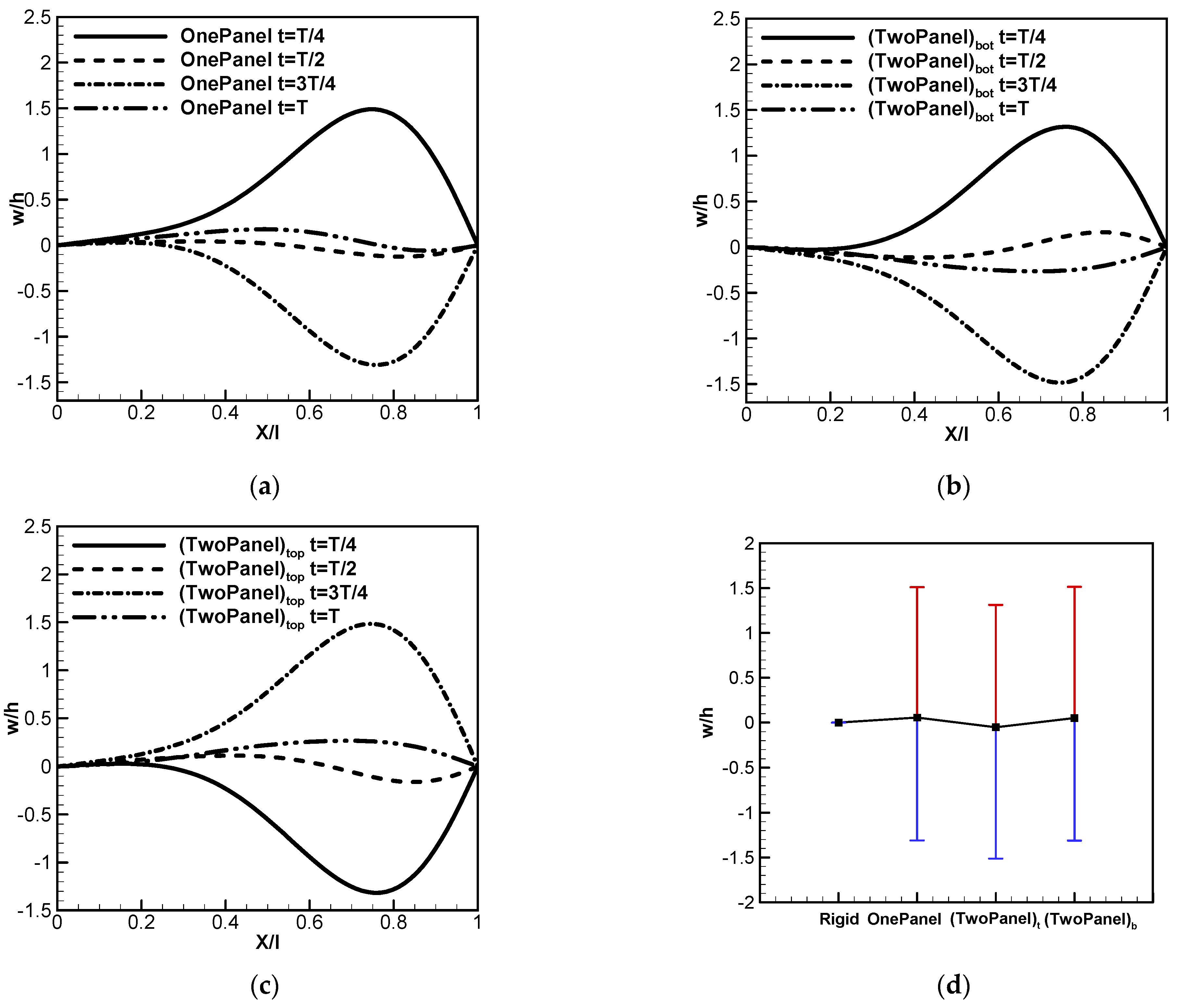
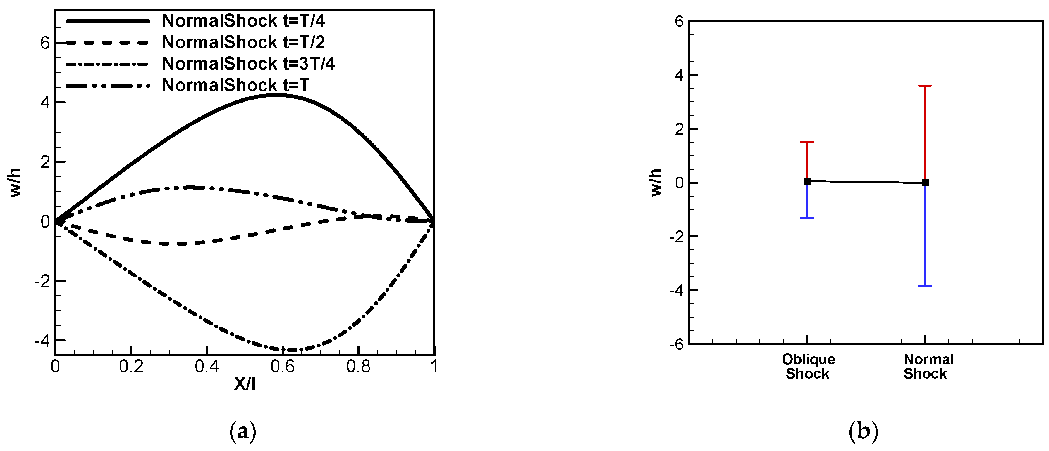
The FSI between thin-walled panels and oblique shock trains induces the LCO of panel structures, with the structural responses exhibiting similar equilibrium positions and flutter amplitudes for all the cases. The panel shapes predominantly manifest as a combination of first- and second-mode responses, with the maximum deflection occurring at 0.75l.

(2)

In Case 1, where one thin-walled panel is positioned at the bottom wall upstream of the oblique shock train, the separation zones and shock structures shift downstream with the decreasing length compared to the rigid wall conditions. While the local flow symmetry level decreases with minor transient fluctuations, the overall flow symmetry level exhibits minor changes with larger transient fluctuations. The isolator performance experiences minor alterations with transient fluctuations.

(3)

In Case 2, with panels at the top and bottom walls upstream of the oblique shock train, the separation zones and shock train structures slightly shift upstream compared to Case 1 but remain downstream of the rigid wall conditions. Although the separation length and shock distance are slightly affected, the transient fluctuations in the separation and shock parameters intensify. The local flow asymmetry increases with more drastic transient fluctuations, while the overall flow symmetry remains similar to Case 1. The isolator performance averages almost the same, with slightly more violent transient fluctuations.

(4)

The FSI effects under normal shock train conditions exert a larger influence on the structural response and isolator flow compared to oblique shock train conditions. The LCO is triggered under normal shock train conditions, with the panel shapes dominated by the first-order mode response, exhibiting larger flutter amplitudes and frequencies. The effects of FSIs under normal shock train conditions on the averaged separation characteristics, shock characteristics, and isolator performance are the opposite (with larger influence) to those under oblique shock train conditions, with significantly more drastic transient fluctuations.

In summary, the influence of FSIs between thin-walled panels and shock trains is significant and complex, triggering different dynamic responses in the panel structures under various conditions. This results in diverse dynamic flow features and isolator performance outcomes. Notably, oblique shock trains demonstrate greater resilience to FSIs compared to normal shock trains. Therefore, FSIs must be meticulously considered in isolator design to prevent engine failure and structural damage. Additionally, elastic structures present a potential strategy for passive flow control in isolators.

References

- Gnani, F.; Zare-Behtash, H.; Kontis, K. Pseudo-shock waves and their interactions in high-speed intakes. Prog. Aerosp. Sci. 2016, 82, 36–56. [Google Scholar] [CrossRef]
- Xu, K.; Chang, J.; Li, N.; Zhou, W.; Yu, D. Preliminary investigation of limits of shock train jumps in a hypersonic inlet-isolator. Eur. J. Mech. 2018, 72, 664–675. [Google Scholar] [CrossRef]
- Urzay, J. Supersonic Combustion in Air-Breathing Propulsion Systems for Hypersonic Flight. Annu. Rev. Fluid Mech. 2018, 50, 593–627. [Google Scholar] [CrossRef]
- Im, S.K.; Do, H. Unstart phenomena induced by flow choking in scramjet inlet-isolators. Prog. Aerosp. Sci. 2018, 97, 1–21. [Google Scholar] [CrossRef]
- Hunt, R.L.; Gamba, M. Shock train unsteadiness characteristics, oblique-to-normal transition, and three-dimensional leading shock structure. AIAA J. 2018, 56, 1569–1587. [Google Scholar] [CrossRef]
- Wang, Z.; Xin, X.; Guo, J.; Yue, L.; Kong, C.; Huang, R.; Chang, J. Hysteresis behavior of shock train driven by continuous incoming Mach number variation in an isolator with background waves. Eur. J. Mech. 2023, 101, 42–58. [Google Scholar] [CrossRef]
- Zheng, K.; Tian, W.; Qin, J.; Zhang, S.; Hu, H. Effect of film cooling injection on aerodynamic performances of scramjet isolator. Aerosp. Sci. Technol. 2019, 94, 150383. [Google Scholar] [CrossRef]
- Vanstone, L.; Hashemi, K.E.; Lingren, J.; Akella, M.R.; Clemens, N.T.; Donbar, J.; Gogineni, S. Closed-loop control of shock-train location in a combusting scramjet. J. Propuls. Power 2018, 34, 660–667. [Google Scholar] [CrossRef]
- Xing, F.; Ruan, C.; Huang, Y.; Fang, X.; Yao, Y. Numerical investigation on shock train control and applications in a scramjet engine. Aerosp. Sci. Technol. 2017, 60, 162–171. [Google Scholar] [CrossRef]
- McNamara, J.J.; Friedmann, P.P. Aeroelastic and Aerothermoelastic Analysis in Hypersonic Flow: Past, Present, and Future. AIAA J. 2011, 49, 1089–1122. [Google Scholar] [CrossRef]
- Liguore, S.; Tzong, G. Identification of Knowledge Gaps in the Predictive Capability for Response and Life Prediction of Hypersonic Vehicle Structures. In Proceedings of the 52nd AIAA/ASME/ASCE/AHS/ASC Structures, Structural Dynamics and Materials Conference, Denver, CO, USA, 4–7 April 2011; pp. 1–9. [Google Scholar] [CrossRef]
- Meng, X.; Ye, Z.; Hong, Z.; Ye, K. Influences of wall vibration on shock train structures and performance of two-dimensional rectangular isolators in scramjet engine. Acta Astronaut. 2020, 166, 180–198. [Google Scholar] [CrossRef]
- Meng, X.; Ye, Z.; Hong, Z.; Ye, K. Impacts of panel vibration on shock train structures and performance of two-dimensional isolators. Aerosp. Sci. Technol. 2020, 104, 105978. [Google Scholar] [CrossRef]
- Meng, X.; Ye, Z.; Ye, K. Effects of flexible panels on normal shock trains and performance of scramjet isolators. Aerosp. Sci. Technol. 2021, 110, 106455. [Google Scholar] [CrossRef]
- Ye, K.; Ye, Z.; Zhang, Q.; Qu, Z. Effects of aeroelasticity on the performance of hypersonic inlet. Proc. Inst. Mech. Eng. Part G J. Aerosp. Eng. 2018, 232, 2108–2121. [Google Scholar] [CrossRef]
- Ye, K.; Ye, Z.; Li, C.; Wu, J. Effects of the aerothermoelastic deformation on the performance of the three-dimensional hypersonic inlet. Aerosp. Sci. Technol. 2019, 84, 747–762. [Google Scholar] [CrossRef]
- Ye, K.; Feng, Z.; Liu, X.; Ye, Z. Numerical investigation of the influence of aerothermoelastic dynamic response on the performance of the three-dimensional hypersonic inlet. Proc. Inst. Mech. Eng. Part G J. Aerosp. Eng. 2022, 236, 2131–2147. [Google Scholar] [CrossRef]
- Matsuo, K.; Miyazato, Y.; Kim, H.D. Shock train and pseudo-shock phenomena in internal gas flows. Prog. Aerosp. Sci. 1999, 35, 33–100. [Google Scholar] [CrossRef]
- Carroll, B.F.; Dutton, J.C. Characteristics of Multiple Shock Wave/Turbulent Boundary-Layer Interactions in Rectangular Ducts. J. Propuls. Power 1989, 6, 186–193. [Google Scholar] [CrossRef]
- Nill, L.; Mattick, A. An experimental study of shock structure in a normal shock train. In Proceedings of the 34th Aerospace Sciences Meeting and Exhibit, Reno, NV, USA, 15–18 January 1996; p. 799. [Google Scholar]
- Miyazato, Y.; Matsuo, K.; Kasada, R. Experimental and Theoretical Investigations of Normal Shock Wave/Turbulent Boundary-Layer Interactions at Low Mach Numbers in a Square Straight Duct. In Proceedings of the 47th AIAA Aerospace Sciences Meeting including the New Horizons Forum and Aerospace Exposition, Orlando, FL, USA, 5–8 January 2009; p. 925. [Google Scholar]
- Ikui, T.; Matsuo, K.; Nagai, M.; Honjo, M. Oscillation phenomena of pseudo-shock waves. Bull. JSME 1974, 17, 1278–1285. [Google Scholar] [CrossRef]
- Klomparens, R.L.; Driscoll, J.F.; Gamba, M. Unsteadiness characteristics and pressure distribution of an oblique shock train. In Proceedings of the 53rd AIAA Aerospace Sciences Meeting, Kissimmee, FL, USA, 5–9 January 2015. [Google Scholar]
- Seleznev, R.K.; Surzhikov, S.T.; Shang, J.S. A review of the scramjet experimental data base. Prog. Aerosp. Sci. 2019, 106, 43–70. [Google Scholar] [CrossRef]
- Eason, T.G.; Spottswood, S. A Structures Perspective on the Challenges Associated with Analyzing a Reusable Hypersonic Platform. In Proceedings of the 54th AIAA/ASME/ASCE/AHS/ASC Structures, Structural Dynamics, and Materials Conference, Boston, MA, USA, 8–11 April 2013. [Google Scholar] [CrossRef]
- Dowell, E.H. Nonlinear oscillations of a fluttering plate. AIAA J. 1966, 4, 1267–1275. [Google Scholar] [CrossRef]
- Dowell, E.H. Nonlinear oscillations of a fluttering plate. II. AIAA J. 1967, 5, 1856–1862. [Google Scholar] [CrossRef]
- Dowell, E.H. Panel flutter—A review of the aeroelastic stability of plates and shells. AIAA J. 1970, 8, 385–399. [Google Scholar] [CrossRef]
- Mei, C.; Abdel-Motagaly, K.; Chen, R. Review of Nonlinear Panel Flutter at Supersonic and Hypersonic Speeds. Appl. Mech. Rev. 1999, 52, 321–332. [Google Scholar] [CrossRef]
- Meng, X.; Ye, Z.; Liu, C. Nonlinear Analysis on Piston Theory. AIAA J. 2019, 57, 4583–4587. [Google Scholar] [CrossRef]
- Meng, X.; Ye, Z.; Ye, K.; Liu, C. Aerodynamic Nonlinearity of Piston Theory in Surface Vibration. J. Aerosp. Eng. 2020, 33, 04020035. [Google Scholar] [CrossRef]
- Meng, X.; Ye, Z.; Ye, K.; Liu, C. Analysis on location of maximum vibration amplitude in panel flutter. Proc. Inst. Mech. Eng. Part G J. Aerosp. Eng. 2020, 234, 457–469. [Google Scholar] [CrossRef]
- Spottswood, S.M.; Eason, T.G.; Beberniss, T. Influence of shock-boundary layer interactions on the dynamic response of a flexible panel. In Proceedings of the International Conference on Noise and Vibration Engineering 2012, Leuven, Belgium, 17–19 September 2012; pp. 603–616. [Google Scholar]
- Spottswood, S.M.; Beberniss, T.J.; Eason, T.G.; Perez, R.A.; Donbar, J.M.; Ehrhardt, D.A.; Riley, Z.B. Exploring the response of a thin, flexible panel to shock-turbulent boundary-layer interactions. J. Sound Vib. 2019, 443, 74–89. [Google Scholar] [CrossRef]
- Daub, D.; Willems, S.; Gülhan, A. Experimental results on unsteady shock-wave/boundary-layer interaction induced by an impinging shock. CEAS Space J. 2016, 8, 3–12. [Google Scholar] [CrossRef]
- Willems, S.; Gülhan, A.; Esser, B. Shock induced fluid-structure interaction on a flexible wall in supersonic turbulent flow. Prog. Flight Phys. 2013, 5, 285–308. [Google Scholar] [CrossRef]
- Daub, D.; Willems, S.; Gulhan, A. Experiments on the interaction of a fast-moving shock with an elastic panel. AIAA J. 2016, 54, 670–678. [Google Scholar] [CrossRef]
- Visbal, M. Viscous and inviscid interactions of an oblique shock with a flexible panel. J. Fluids Struct. 2014, 48, 27–45. [Google Scholar] [CrossRef]
- Ye, L.-Q.; Ye, Z.-Y. Effects of Shock Location on Aeroelastic Stability of Flexible Panel. AIAA J. 2018, 56, 3732–3744. [Google Scholar] [CrossRef]
- Ye, L.; Ye, Z. Aeroelastic Stability Analysis of Heated Flexible Panel in Shock-Dominated Flows. Chin. J. Aeronaut. 2018, 31, 1650–1666. [Google Scholar] [CrossRef]
- Quan, E.; Xu, M.; Yao, W.; Cheng, X. Analysis of the post-flutter aerothermoelastic characteristics of hypersonic skin panels using a CFD-based approach. Aerosp. Sci. Technol. 2021, 118, 107076. [Google Scholar] [CrossRef]
- Daub, D.; Willems, S.; Gülhan, A. Experiments on aerothermoelastic fluid–structure interaction in hypersonic flow. J. Sound Vib. 2022, 531, 116714. [Google Scholar] [CrossRef]
- Yao, C.; Zhang, G.H.; Liu, Z.S. Forced shock oscillation control in supersonic intake using fluid-structure interaction. AIAA J. 2017, 55, 2580–2596. [Google Scholar] [CrossRef]
- Liu, W.; Wu, Y.; Li, Y.; Chen, X. Effect of cavity pressure on shock train behavior and panel aeroelasticity in an isolator. Phys. Fluids 2022, 34, 126101. [Google Scholar] [CrossRef]
- Thompson, M.K.; Thompson, J.M. ANSYS Mechanical APDL for Finite Element Analysis; Butterworth-Heinemann: Oxford, UK, 2017. [Google Scholar]
- Gaitonde, D.V. Progress in shock wave/boundary layer interactions. Prog. Aerosp. Sci. 2015, 72, 80–99. [Google Scholar] [CrossRef]
- Gnani, F.; Zare-Behtash, H.; White, C.; Kontis, K. Numerical investigation on three-dimensional shock train structures in rectangular isolators. Eur. J. Mech. B Fluids 2018, 72, 586–593. [Google Scholar] [CrossRef]
- Sun, L.; Sugiyama, H.; Mizobata, K.; Minato, R.; Tojo, A. Numerical and Experimental Investigation on Shock Wave and Turbulent Boundary Layer Interactions in a Square Duct at Mach 2 and 4. Japan Soc. Aeronaut. Sp. Sci. 2004, 47, 124–130. [Google Scholar]
- Li, N. Response of Shock Train to Fluctuating Angle of Attack in a Scramjet Inlet-Isolator. Acta Astronaut. 2022, 190, 430–443. [Google Scholar] [CrossRef]
- Zhou, H.; Wang, G.; Li, Q.; Liu, Y. Numerical Study on the Nonlinear Characteristics of Shock Induced Two-Dimensional Panel Flutter in Inviscid Flow. J. Sound Vib. 2023, 117893. [Google Scholar] [CrossRef]
- Boyer, N.R.; McNamara, J.J.; Gaitonde, D.V.; Barnes, C.J.; Visbal, M.R. Features of Panel Flutter Response to Shock Boundary Layer Interactions. J. Fluids Struct. 2021, 101, 103207. [Google Scholar] [CrossRef]
- Gordnier, R.E.; Visbal, M.R. Development of a Three-Dimensional Viscous Aeroelastic Solver for Nonlinear Panel Flutter. J. Fluids Struct. 2002, 16, 497–527. [Google Scholar] [CrossRef]